www.atmos-chem-phys.net/16/8125/2016/ doi:10.5194/acp-16-8125-2016
© Author(s) 2016. CC Attribution 3.0 License.
The millennium water vapour drop in chemistry–climate
model simulations
Sabine Brinkop1, Martin Dameris1, Patrick Jöckel1, Hella Garny1, Stefan Lossow2, and Gabriele Stiller2
1Deutsches Zentrum für Luft- und Raumfahrt (DLR), Institut für Physik der Atmosphäre, Oberpfaffenhofen, Germany 2Karlsruher Institut für Technologie (KIT), Institut für Meteorologie und Klimaforschung, Karlsruhe, Germany
Correspondence to:Sabine Brinkop ([email protected])
Received: 11 August 2015 – Published in Atmos. Chem. Phys. Discuss.: 14 September 2015 Revised: 25 May 2016 – Accepted: 11 June 2016 – Published: 6 July 2016
Abstract.This study investigates the abrupt and severe wa-ter vapour decline in the stratosphere beginning in the year 2000 (the “millennium water vapour drop”) and other simi-larly strong stratospheric water vapour reductions by means of various simulations with the state-of-the-art Chemistry-Climate Model (CCM) EMAC (ECHAM/MESSy Atmo-spheric Chemistry Model). The model simulations differ with respect to the prescribed sea surface temperatures (SSTs) and whether nudging is applied or not. The CCM EMAC is able to most closely reproduce the signature and pattern of the water vapour drop in agreement with those derived from satellite observations if the model is nudged. Model results confirm that this extraordinary water vapour decline is particularly obvious in the tropical lower strato-sphere and is related to a large decrease in cold point tem-perature. The drop signal propagates under dilution to the higher stratosphere and to the poles via the Brewer–Dobson circulation (BDC). We found that the driving forces for this significant decline in water vapour mixing ratios are tropical sea surface temperature (SST) changes due to a coincidence with a preceding strong El Niño–Southern Oscillation event (1997/1998) followed by a strong La Niña event (1999/2000) and supported by the change of the westerly to the easterly phase of the equatorial stratospheric quasi-biennial oscilla-tion (QBO) in 2000. Correct (observed) SSTs are important for triggering the strong decline in water vapour. There are indications that, at least partly, SSTs contribute to the long period of low water vapour values from 2001 to 2006. For this period, the specific dynamical state of the atmosphere (overall atmospheric large-scale wind and temperature dis-tribution) is important as well, as it causes the observed per-sistent low cold point temperatures. These are induced by a
period of increased upwelling, which, however, has no cor-responding pronounced signature in SSTs anomalies in the tropics. Our free-running simulations do not capture the drop as observed, because a) the cold point temperature has a low bias and thus the water vapour variability is reduced and b) because they do not simulate the appropriate dynamical state. Large negative water vapour declines are also found in other years and seem to be a feature which can be found after strong combined El Niño/La Niña events if the QBO west phase during La Niña changes to the east phase.
1 Introduction
Since the early 1980s balloon-borne stratospheric water vapour measurements (e.g. Hurst et al., 2011) and cli-mate models have predicted a continuous increase in strato-spheric water vapour concentrations (Stenke and Grewe, 2005; SPARC CCMVal, 2010; Gettelman et al., 2010). Satel-lite measurements have not yet observed such an increase (UARS/MLS, UARS HALOE, and SAGE II instruments; see for instance Solomon et al., 2010; Hartmann et al., 2013). However, if we look from the late 1980s/early 1990s to now, we actually find a decreasing trend from merged satellite ob-servations in the lower stratosphere (see Hegglin et al., 2014). The explanation for this has become a large scientific chal-lenge and a lot of discussion persists on whether Boulder bal-loon observations are representative or if there is an issue in the satellite data merging.
However, multi-year data sets show significant fluctuations on different timescales, which makes it difficult to assess ro-bust trends (Hegglin et al., 2014).
In the year 2000, an extraordinary sudden drop of strato-spheric water vapour content was observed (e.g. Ran-del et al., 2006; Fueglistaler et al., 2005; Rosenlof and Reid, 2008; Maycock et al., 2014), which again brought into focus that temperature fluctuations have a large poten-tial to significantly impact the amount of water vapour in the stratosphere. The strong and widely noticed water vapour drop in the year 2000 is particularly remarkable due to the fact that it is followed by a 5-year period of low strato-spheric humidity. Randel and colleagues showed that the tropical tropopause temperatures remain noticeably lower than normal after the decline due to an increase in tropical upwelling. The lowest temperatures after the drop lie over the western tropical Pacific/Indonesia region and Africa dur-ing all seasons of the year, but are not a major feature in the Caribbean or the mid-Pacific (Rosenlof and Reid, 2008). Solomon et al. (2010) found that stratospheric water vapour concentrations decreased by about 10 % after the year 2000. They showed that “this acted to slow the rate of increase in global surface temperature over 2000–2009 by about 25 % compared to that which would have occurred due only to car-bon dioxide and other greenhouse gases.”
Since water vapour is the most prominent greenhouse gas, and therefore is an important contributor to variations and trends in climate, it is necessary to better understand its large variability. Stratospheric water vapour variations are con-nected with temperature changes in the tropical region, espe-cially with the cold point temperature (Randel et al., 2004; Fueglistaler et al., 2013). Changes of stratospheric water vapour levels ranging from interannual to decadal timescales are less well understood, in particular the contribution of processes involved. Well known and understood is the “tape recorder” effect (Mote et al., 1996), describing the annual cycle of the tropical stratospheric water vapour amount in accordance with the seasonally varying cold point temper-ature (e.g. Fueglistaler et al., 2005). Moreover, variations of the tropopause temperatures are clearly related to trop-ical upwelling, the equatorial quasi-biennial oscillation of stratospheric zonal winds (QBO), and the El Niño–Southern Oscillation (ENSO) as, for example, discussed by Randel et al. (2004). Recent analyses of the observed stratospheric water vapour record show that many of the variations on timescales of 1 to several years can be linked to changes in tropical tropopause temperatures, but some discrepancies still exist (e.g. Schoeberl et al., 2012; Fueglistaler et al., 2013). Randel and Jensen (2013) state that the water vapour fluctuations observed by satellite instruments over the last 20-years are not adequately reproduced by “free-running” CCMs, although those were forced by observed sea-surface temperatures (SSTs) and concentrations of greenhouse gases and ozone-depleting substances were prescribed. Randel and Jensen point out that current CCMs are not able to
recon-struct the severe water vapour drop after the beginning of year 2000. Therefore, they conclude that important compo-nents of internal variability might be missing or are at least under-represented in the model systems, especially in the tropical tropopause layer (TTL). Similar investigations sum-marize that it is still unclear whether the inability to simulate the observed trends is due to the large uncertainties in the observed stratospheric water vapour and tropical tropopause temperatures (e.g. Wang et al., 2012), inaccuracies in the CCMs, or whether the models miss relevant mechanisms (see Chap. 4 in WMO, 2014).
Here we present results of a set of four simulations with different model set-ups with the state-of-the-art CCM EMAC (ECHAM/MESSy Atmospheric Chemistry model), indicat-ing that it is possible to retrace the observed water vapour fluctuations in the stratosphere (including the millennium drop). In the following section the CCM EMAC is briefly described, the investigated model simulations and the used observational data sets are presented. The millennium water vapour drop as represented in one of the model simulations is compared to observations in Sect. 3. To clarify which part of the millennium drop we refer to, we define two differ-ent phases of “the drop”: phase 1 is the short period of the steep decline between the drop onset, i.e. the water vapour maximum and its subsequent minimum. Phase 2 is the pe-riod of low values between the minimum and the start of the recovery. In Sect. 4 all model simulations are compared with respect to their ability to represent the millennium drop. Sec-tion 5 provides an analysis of other large moisture anomalies in the lower stratosphere and their relation to preceding El Niño/La Niña events. An overall discussion of our findings is given in Sect. 6.
2 Method and data
2.1 Description of the model system
The ECHAM/MESSy Atmospheric Chemistry (EMAC) model is a numerical chemistry and climate simulation sys-tem that includes submodels describing tropospheric and middle atmosphere processes and their interaction with oceans, land, and human influences (Jöckel et al., 2010). It uses the second version of the Modular Earth Submodel Sys-tem (MESSy2) to link multi-institutional computer codes. The core atmospheric model is the fifth-generation Euro-pean Centre Hamburg general circulation model (ECHAM5, Roeckner et al., 2006). For the present study we analysed EMAC (ECHAM5 version 5.3.02, MESSy version 2.50) in the T42L90MA-resolution, i.e. with a spherical truncation of T42 (corresponding to a quadratic Gaussian grid of approx. 2.8 by 2.8◦in latitude and longitude) with 90 vertical hybrid
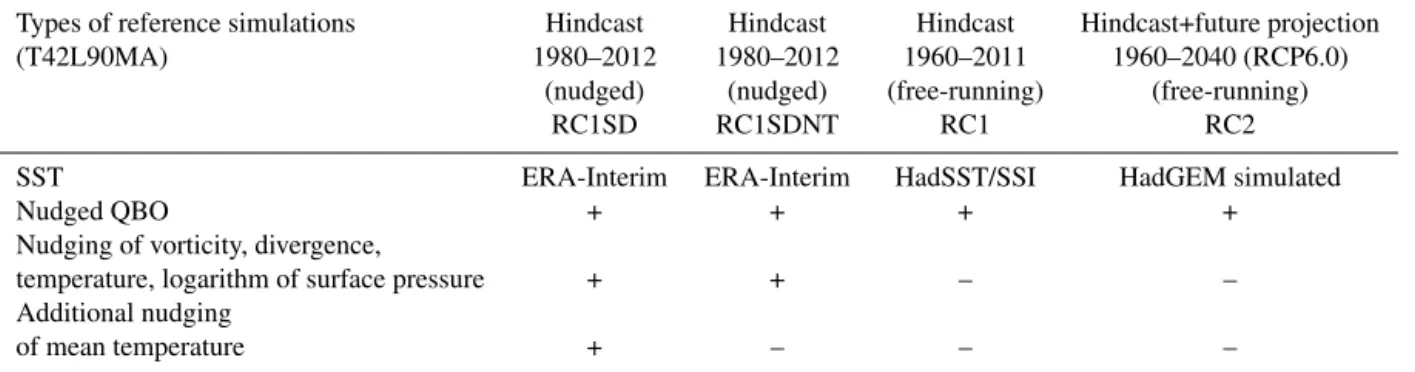
Table 1.Overview over the chemistry–climate model simulations used for this analysis.
Types of reference simulations Hindcast Hindcast Hindcast Hindcast+future projection
(T42L90MA) 1980–2012 1980–2012 1960–2011 1960–2040 (RCP6.0)
(nudged) (nudged) (free-running) (free-running)
RC1SD RC1SDNT RC1 RC2
SST ERA-Interim ERA-Interim HadSST/SSI HadGEM simulated
Nudged QBO + + + +
Nudging of vorticity, divergence,
temperature, logarithm of surface pressure + + – –
Additional nudging
of mean temperature + – – –
The multi-year simulations have been performed with the CCM EMAC in the framework of the ESCiMo project (Earth System Chemistry integrated Modelling, Jöckel et al., 2016). Within ESCiMo, so-called reference simulations (RCs) have been carried out, as defined by the IGAC/SPARC Chemistry-Climate Model Initiative (CCMI) and described in detail by Eyring and Lamarque (2012). The forcing of the transient reference simulations in either free-running (RC1; from 1960 to 2011) or nudged mode (RC1SD, RC1SDNT; from 1980 to 2012) are similar (hindcast simulations). They are taken from observations or empirical data, including anthropogenic and natural forcing based on changes in trace gases, solar vari-ability, and volcanic eruptions (see Table 1 for an overview). The sea surface temperatures (SSTs) and the sea ice con-centrations (SICs) are from observations or reanalysis data (RC1: HadISST, RC1SD and RC1SDNT: ERA-Interim. In the case of RC1SD, the model prognostic variables (vorticity, divergence, the logarithm of the surface pressure, the temper-ature, and additionally the mean temperature – wave number zero in spectral space) are nudged by Newtonian relaxation towards ERA-Interim reanalysis data. RC1SDNT is nudged similarly with the exception that the mean temperature is
notnudged. The transient forecast reference simulation RC2 (from 1960 to 2100) is a future projection that follows the IPCC scenario RCP 6.0 and a specified scenario of the devel-opment of ozone-depleting substances (halogen scenario A1 from Table 5-A3 of the World Meteorological Organisation (WMO), 2011). It also considers solar variability in the past and future (for details see Jöckel et al., 2016). Because of potential discontinuities between the observed and simulated data record, RC2 uses SSTs and SICs derived from a cou-pled climate model simulation (with an interactive ocean, HadGEM2 (Hadley Centre Global Environment Model ver-sion 2), RCP6.0 scenario; Jones et al., 2011) for the entire period. In the following analysis we confine the data of the RC2 simulation from 1960 to 2040.
The internal generation of a QBO is a feature of the L90MA set-up of EMAC (Giorgetta et al., 2002). Therefore, in all simulations a QBO is internally generated. Neverthe-less, the zonal winds near the equator are nudged towards a zonal mean field with a Gaussian profile in the latitudinal
direction and with a relaxation timescale of 58 days in our simulations to get the correct phasing of the observed QBO (Jöckel et al., 2016). The nudging is applied in the altitude range between 10–90 hPa, with full nudging weights (i.e. 1.0) from 20–50 hPa, levelling off to 0.3 (0.2) at the upper (lower) edge of the nudging region. Full nudging is utilized between 7◦S–7◦N latitudes. As can be seen in Fig. S1
(Supple-ment), this does not necessarily mean that the QBO is equal in all simulations! The nudged model simulations (RC1SD, RC1SDN) better represent the observed zonal mean wind component in amplitude and absolute values compared to the observed winds (Singapore radiosonde). RC1 and RC2 sim-ulate the QBO at 90 hPa only poorly, but capture to some extend the variability at 70 hPa.
2.2 Observational data sets
For comparison with our EMAC simulation with specified dynamics RC1SD (nudged mode), we use (i) the water vapour data from combined HALOE (Halogen Occultation Experiment) and MLS satellite measurements as described in Randel and Jensen (2013), (ii) a merged data set from seven limb-viewing satellite instruments, which were compiled into a long-term record (Hegglin et al., 2014), and (iii) a com-bination of satellite observations performed by HALOE and MIPAS (Michelson Interferometer for Passive Atmospheric Sounding) instruments (Russell et al., 1993; Fischer et al., 2008). For more details see the Appendices A1–A3.
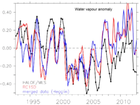
Figure 1. Interannual changes of the near-global mean (60◦S–
60◦N) stratospheric water vapour mixing ratios (in ppmv) at
83 hPa. The black line is the data derived from satellite observa-tions (combined HALOE and Aura/MLS satellite measurements, deseasonalized, 3-month average), which were published by Ran-del and Jensen (2013) in their Fig. 5a (upper graph). The red line is the RC1SD simulation (deseasonalized, 3-month running mean). The blue line is the merged data set as published by Heg-glin et al. (2013). The correlation between HALOE/Aura/MLS and
RC1SD isr=0.68 and between the merged data set and RC1SD
r=0.73. (r: Pearson’s correlation coefficient, see Appendix B).
3 The millennium water vapour drop
This study is motivated by a chart which is shown in Fig. 1 (the original figure was published by Randel and Jensen, 2013): the near-global lower stratospheric water vapour anomalies were derived from multi-year satellite measure-ments (1992–2012) from HALOE and Aura/MLS at the 83 hPa pressure level (approximately 17 km altitude). The measurements impressively indicate interannual fluctuations of up to 15 % (about 0.5 ppmv) in water vapour mixing ratios. There are clear signs of the QBO over the full time period. The figure highlights the severe water vapour drop (approxi-mately−0.7 ppmv) in the year 2000.
The HALOE data (see Fig. 1) show a step-like change from an enhanced water vapour period before the drop (1993–2000) into a phase with reduced water vapour. The re-covery from this phase (our phase 2) with prevailing negative anomalies starts in 2007. The RC1SD simulation (nudged, including mean temperature nudging) closely reproduces the water vapour fluctuations as observed. The timing of relative minimum and maximum water vapour values is reproduced very well. Evidently the model underestimates the strength of the interannual fluctuations (only about 0.3 ppmv instead of 0.5 ppmv) compared to the combined HALOE/Aura-MLS satellite data. The amplitude of the severe drop (phase 1) in 2000 is by about 0.12 ppmv smaller than in the combined HALOE/Aura-MLS satellite data, yet the period with lower than normal water vapour (phase 2) is captured well. The deviation of the RC1SD simulation results from the merged data set by Hegglin et al. (2014) (see Fig. 1) is even smaller.
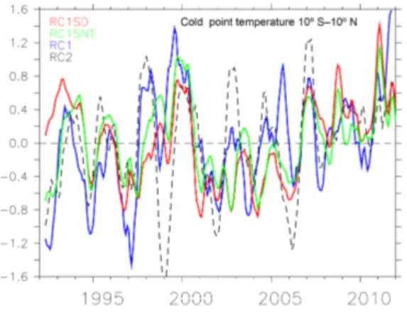
Figure 2.Cold point temperature anomalies in the tropics (20◦S–
20◦N) derived from radiosonde data (black line). The data were
al-ready published by Randel and Jensen (2013) in their Fig. 5a (lower graph). The red line is the RC1SD simulation (deseasonalized,
3-month running mean). The correlation coefficient isr=0.61.
RC1SD and the merged data set agree in particular with re-spect to (a) the start of the recovery phase after the drop, which starts earlier as in the HALOE data, (b) the ampli-tude of the drop, and (c) the lower water vapour anomalies in the period before the drop. The merged data set consists of individual short satellite records, merged with the simu-lated water vapour from a chemistry–climate model, which was nudged to observed meteorology. For the lower strato-sphere this record of water vapour mixing ratios largely fol-lows tropical tropopause temperatures. This might be the rea-son why the RC1SD and the merged data set are in better agreement.
Figure 2 (also corresponding to Fig. 2 of Randel and Jensen, 2013) moreover shows that the cold point temper-ature anomalies of RC1SD follow those of the radiosonde data. This can be expected due to the nudging of EMAC to-wards ERA-Interim data.
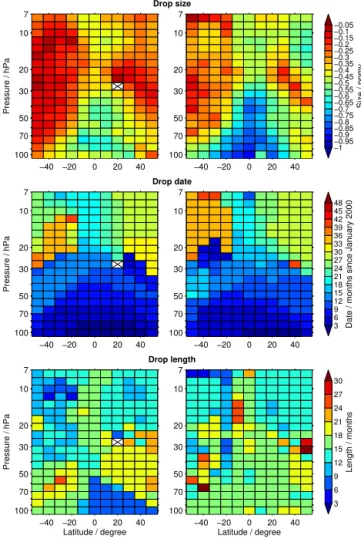
There are expectations that the water vapour drop in ob-servations exhibits different characteristics at different lati-tudes and altilati-tudes with respect to the start date, the drop size (amplitude), and the length (duration) of the anomaly. For example, Urban et al. (2014) showed that in the tropics the significant reduction of water vapour started in the alti-tude range from 16.5 to 18.5 km (375–425 K) in early 2000, whereas it began between 25 and 30 km (625–825 K) in late 2001. Moreover, they demonstrated that the drop was more pronounced in the lower tropical stratosphere than in the mid-dle stratosphere, i.e.−1.3 and−0.6 ppmv respectively. The minimum water vapour mixing ratios were found in the lower stratosphere about 1 year, in the middle stratosphere almost 2 years after the onset of the drop.
−40 −20 0 20 40 7 10 20 30 50 70 100
Pressure / hPa
−40 −20 0 20 40 7 10 20 30 50 70 100
Pressure / hPa
−40 −20 0 20 40 7 10 20 30 50 70 100
Latitude / degree
Pressure / hPa
−1 −0.95 −0.9 −0.85 −0.8 −0.75 −0.7 −0.65 −0.6 −0.55 −0.5 −0.45 −0.4 −0.35 −0.3 −0.25 −0.2 −0.15 −0.1 −0.05
Size / ppmv
−40 −20 0 20 40 7 10 20 30 50 70 100 3 6 9 12 15 18 21 24 27 30 33 36 39 42 45 48
Date / months since January 2000
−40 −20 0 20 40 7 10 20 30 50 70 100 3 6 9 12 15 18 21 24 27 30
Length / months
−40 −20 0 20 40 7 10 20 30 50 70 100
Latitude / degree
Drop size
Drop date
Drop length
Figure 3.Characteristics of the millennium water vapour decline (phase 1) with respect to height (hPa). The analysis approach of the water vapour decline is described in the Appendix A4. Right: satel-lite observations. Left: RC1SD simulation. Top: drop size (ampli-tude)(unit: ppmv), middle: drop date (months since January 2000), bottom: drop length (duration) (unit: months). White boxes with crosses indicate that the analysis failed to find a water vapour de-crease that fulfilled the criteria listed in the Appendix A4.
and altitude for both, the combined HALOE/MIPAS data set (Schieferdecker, 2015) and for the RC1SD simulation. The details of the methodology are described in Appendix A4.
The amplitude (drop size) of the drop consistently maxi-mizes in the tropical lower stratosphere in observations and the RC1SD simulation (Fig. 3, top). However, the amplitude in the tropics is larger in the observations. Towards higher latitudes and altitudes up to about 20 hPa the drop ampli-tude typically decreases. Above this level some increase in the drop amplitude can be observed that goes along with a stronger QBO variability. It is unclear if the drop amplitude here can be unambiguously attributed to the millennium drop or simply reflects natural QBO variability or a combination of both.
Figure 4.Near-global mean (60◦S–60◦N) water vapour anomalies (in ppmv) (deseasonalized; note, these anomalies are a 12-month running mean and therefore slightly different compared to RC1SD in Fig. 1) derived from RC1SD, RC1SDNT, RC1, and RC2 simula-tions.
A similar pattern can be seen for the start date of the millennium drop (Fig. 3, middle). Up to 40 hPa the drop occurs in most cases during the year 2000. Above 30 hPa there is a clear shift to dates in 2002 and 2003, again mostly controlled by QBO variability. The stronger branch of the Brewer–Dobson circulation in the Northern Hemisphere is clearly visible in the earlier start dates of the drop compared to the Southern Hemisphere.
The duration of phase 1 is the less consistent quantity (Fig. 3, bottom). Values typically range from 6 months (in-herent from the approach) to about 20 months. In the sim-ulation the length is in the order of 9 months in the low-ermost tropical stratosphere. The observations exhibit here longer drops related to the larger drop amplitudes.
In conclusion, Fig. 3 nicely reflects that the cold point tropopause anomaly reduces water vapour and that this sig-nal propagates into the upper stratosphere and further to the poles. The propagation is a bit asymmetric due to the differ-ent branches of the Brewer–Dobson circulation.
4 The millennium water vapour drop in other ESCiMo simulations
In the last section, we showed that the millennium water vapour drop is reasonably well reproduced by the RC1SD simulation with nudged mean temperature. In the follow-ing we investigate whether the other simulations RC1SDNT, RC1, and RC2 (see Table 1) are also capable of simulating the variability of lower stratospheric water vapour and, in particular, the drop in the year 2000.
tempera-Figure 5.Cold point temperature anomalies (K; deseasonalized, 12-month running mean) derived from RC1SD, RC1SDNT, RC1, and RC2 simulations.
ture anomalies (Fig. 5) are in better agreement with RC1SD. Since RC1SD and RC1SDNT differ only with respect to the nudging of the global mean temperature, the RC1SD sim-ulation implies a bias correction and RC1SDNT is affected by this bias. Therefore, the smaller water vapour anomaly amplitude in RC1SDNT is likely caused by a tropical cold point temperature of 189.4 K, which is biased low compared to that of RC1SD (192.1 K) within the 1992–2012 period. Contemporary CCMs show a large spread of about 10 K in simulating cold point tropopause temperatures (Gettelman et al., 2009). This corresponds to the similar wide spread of simulated ozone at the tropopause level and to differently simulated tropopause altitudes. Since the cold point tempera-ture strongly affects stratospheric water vapour, we conclude that in order to correctly simulate water vapour anomalies in time and amplitude, it is not sufficient to reproduce the temperature anomaly. The mean cold point temperature must be simulated correctly as well. The explanation for this is the non-linear dependence of water vapour on temperature as de-scribed by the Clausius–Clapeyron equation.
The magnitude of interannual variability in water vapour in the tropical lower stratosphere is overall far lower in the free-running simulation RC1 (Fig. 4). We will discuss and quantify this at the end of this section. However, a decrease in water vapour around the year 2000 is found also in RC1. The strength of the drop (phase 1) is underestimated by a fac-tor of 2. The minimum period (phase 2) is visible but the minimum is far too high. Compared to RC1SDNT, the free-running RC1 simulation does not simulate the observed at-mospheric dynamical state. Yet, this also seems to be impor-tant for reproducing the observed water vapour variability, in particular the millennium drop. This is consistent with the results of Garfinkel et al. (2013b), who showed, with model simulations forced by observed SSTs only, that SSTs alone cannot explain the timing and the subsequent recovery of the millennium drop.
Figure 6.Saturation water vapour anomaly over ice (deseasonal-ized, 6-month running mean) calculated from the respective cold
point temperatures (10◦S–10◦N) of RC1SD and RC1 simulations.
RC1 shifted: mean cold point temperature of RC1 is shifted to RC1SD mean cold point temperature. The mean cold point tem-peratures are RC1SD: 192.1 K and RC1: 186.0 K (RC1 shifted: 192.1 K).
The main difference between the RC2 and RC1 simulation is that RC2 uses simulated instead of observed SSTs. Be-cause of this difference, RC2 shows neither the water vapour decline nor the long period with low water vapour values af-ter 2000. Accordingly, no low cold point temperature anoma-lies are visible in Fig. 5.
The effect of the correct cold point temperature on the sat-uration water vapour value is also demonstrated for the RC1 simulation (Fig. 6). We took the temperature variability of RC1 as shown in Fig. 5, but used the actual cold point mean temperature as simulated in RC1SD. Thus, we shifted the cold point temperature anomalies. Then we calculated the corresponding saturation moisture over ice for RC1SD (just for comparison), for RC1 (original simulation) and for RC1 shifted (shifted cold point temperature anomaly). The results show that a corrected absolute cold point temperature of RC1 (i.e. RC1 shifted) is expected to improve the representation of phase 2 of the drop.
Figure 7.Moisture anomalies in ppmv (detrended, deseasonalized, 12-months running mean) derived from RC1SD and RC1 simula-tions at 80 hPa. Black vertical lines mark strong El Niño events (see Fig. 8) and red asterisks mark the respective subsequent wa-ter vapour drop.
5 Other large negative moisture anomalies (phase 1) in the lower stratosphere and their relation to
preceding El Niño/La Niña events
In this section we analyse other sudden stratospheric water vapour declines (phase 1) and try to understand what they have in common with phase 1 of the millennium drop. In particular, we examine the role of preceding El Niño/La Niña events, related upwelling anomalies and the QBO.
It is well understood that El Niño/La Niña events have the potential to affect stratospheric variability through SST anomalies (Scaife et al., 2003; Randel et al., 2009; Calvo et al., 2010; Garfinkel et al., 2013a). The La Niña event which started in the autumn of 1998 (after the unusually strong El Niño in 1997/1998) was quite unusual in its duration and in-tensity. Strong La Niña conditions were present for 2 straight years (both the winters of 1998/1999 and 1999/2000 were strong La Niña). It did not fully decay until the summer of 2001, though it was largely gone by spring of 2000 (when the drop started). In the tropical lower stratosphere, the QBO is the dominant dynamic feature (Rosenlof and Reid, 2008; Dessler et al., 2014) which contributes to the extraordinary temperature fluctuation in the tropical tropopause region. It appears as a reversal of the tropical zonal wind direction with a mean period of about 28 months (ranging from 22 to 34 months) and is a primarily wave-driven stratospheric phenomenon.
We have analysed the time evolution of water vapour anomalies for the RC1SD and RC1 simulations at 80 hPa (Fig. 7) for the full time period available for the respective simulations. In the RC1 simulation we found five relatively large water vapour declines, (phase 1) marked by a red
as-Figure 8. (a) Surface temperature anomaly in the tropical
re-gion (10◦S–10◦N) (detrended, deseasonalized, 12-point running
mean) for RC1SD (black), RC1 (red), and RC2 (green). Strong El
Niño/La-Niña events are labelled.(b)Surface temperature (degrees
Celsius) for RC1SD, RC1 and RC2 (12-point running mean).
terisk, and in the RC1SD simulation we found three, which are comparable to the millennium drop amplitude in the re-spective simulation. An additional asterisk marks a smaller water vapour decline after the 1986/1987 El Niño in RC1SD, which was additionally examined. Because the amplitudes in the RC1 simulation are generally smaller than in RC1SD, we define a “large decline” in the simulations differently: RC1SD decline >0.5 ppmv and RC1 decline >0.2 ppmv. The thresholds have been only used to simplify the search of decline events with preceding ENSO events. Thus, the result of event identification counting is independent of the selected values. We could have also started with the ENSO index and searched for decline events after La Niña events. The result is the same.
Although there are two other large water vapour de-clines in the RC1SD simulation starting in 1994 and 1996, we neglect this time period, because the eruption of Mt. Pinatubo (1991) had a significant impact on temperature and water vapour in our simulations (Löffler et al., 2016). Likewise, we cannot exclude that the eruption of Mt. Chi-chon in 1982, although less strong than the eruption of Mt. Pinatubo, had an influence on the results.
The dominant effect of El Niño/La Niña events on the tropical surface temperatures (including land and sea sur-face temperatures) are clearly visible in Fig. 8a in all sim-ulations. The data derived from the RC1 simulation indi-cate strong temperature signals related to the El Niño and La Niña episodes (1: 1969/1970, 2: 1973/1974, 3: 1982/1983, 4: 1986/1987, 5: 1997/1998, 6: 2009/2010). The RC1SD simu-lation only covers El Niño and La Niña events from no 3 to no 6, but the surface temperatures are similar to RC1.
Figure 9. (a)Temporal evolution of moisture anomalies (ppmv).
(b)Temporal evolution of temperature anomalies (K) in the tropical
region (12-month running mean), derived from the RC1 simulation. Strong El Niño events are labelled similarly to Fig. 8. The altitude range covers the pressure levels from 900 to 30 hPa. The dashed lines mark the region between 100 and 50 hPa.
than in observations (Fig. 8b). However, the simulated sur-face temperature represents similar fluctuations (in magni-tude) as observed, but originates in different periods of time and often with a longer time duration. As mentioned above (Sect. 2), in all four EMAC simulations the QBO is nudged to zonal mean winds with respect to the amplitude and phase. Therefore the signature of the QBO in the tempera-ture anomaly (Fig. 9b, RC1 as representative for all simula-tions), propagating downwards to the TTL, is present in all EMAC simulations (for the RC1SD simulation see Fig. S2 in the Supplement). Although the QBO nudging set-up is equal in all simulations presented, the resulting winds are not the same in RC1SD, RC1, and RC2. The QBO nudging does not force a one-by-one representation of the nudged data by the model, the model still develops its own dynamical state. Note that the QBO at roughly 90 hPa is key for the temperature signal affecting water vapour, i.e. at an altitude, where the QBO nudging strength is already reduced and therefore relies on signal propagation. Only for RC1SD (and RC1SDNT), where divergence and vorticity and the logarithm of the sur-face pressure are also nudged, the wind profiles are close to those of ERA-interim (Fig. S1, Supplement). The RC1 and RC2 simulations, however, show a smaller amplitude and the QBO is less visible at 90 hPa.
Around a strong El Niño event (black vertical lines, Fig. 9b) we find a positive moisture (Fig. 9a) and temperature anomaly throughout the troposphere up to about 100 hPa and subsequent moistening of the lower stratosphere. This result is consistent with the findings of Dessler et al. (2014), who showed by regression analysis that stratospheric entry values
of water vapour increase with tropospheric temperature. El Niño as an important driver of the interannual variability is captured in the tropical tropospheric temperature regressor. In contrast, the effect of La Niña events to increase strato-spheric water vapour as discussed by Garfinkel et al. (2013a) is not captured with the tropospheric temperature regressor, but with the BDC (Brewer–Dobson circulation) regressor.
In Fig. 9, in a narrow layer between 100 and 50 hPa (marked with dashed black lines), a negative temperature anomaly occurs, except for the 1982/1983 El Niño, where a positive QBO phase with warming probably masks this feature. For the 1997/1998 and the 2009/2010 El Niño the cooling is not pronounced, but also visible.
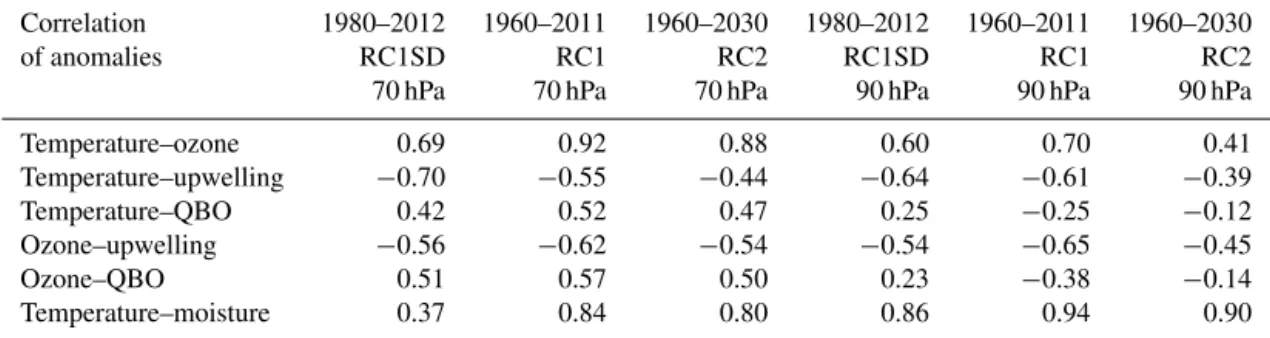
Positive and negative temperature anomalies in the nar-row layer are related by a large part to changes in upwelling (Fig. 10), which directly modifies the tropopause tempera-ture through lifting of air masses. Additionally, a positive upwelling anomaly (cooling) is accompanied by a nega-tive ozone anomaly (cooling; not shown). For this reason upwelling anomaly and ozone anomaly are anti-correlated with a Pearson’s correlation coefficient of aboutr= −0.56 at 70 hPa for both RC1 and RC1SD (Table 2, see Ap-pendix B for the formula of the Pearson’s correlation coef-ficient). Tropical upwelling is calculated from the model re-sults in terms of the residual vertical velocityw∗ as
intro-duced in the transformed Eulerian mean (TEM) equations (e.g. Holton, 2004, his Eq. 10.16b) for the tropics (20◦S–
20◦N). As expected temperature and large-scale upwelling
are also strongly anti-correlated with a Pearson’s correlation coefficientr= −0.7 (70 hPa) for RC1SD (RC1:r= −0.58) (Table 2). Likewise temperature and QBO are positively cor-related withr=0.5 (RC1) (r=0.4 for RC1SD) at 70 hPa. The correlation coefficient decreases at lower altitudes, be-cause the effect of the QBO on temperature decreases.
In the TTL, positive temperature anomalies always result in positive water vapour anomalies propagating upwards into the stratosphere (Fig. 9). This is independent of a heating and moistening of the tropical troposphere during El Niños and also occurs under La Niña conditions. Because El Niño (La Niña) conditions lead to an increase (decrease) in up-welling (Fig. 9) a cooling (warming) of the TTL region can often be found (El Niños 1, 2, 4, 5, 6, La Niñas: 2, 4, 5, 6). A moistening can occur in cases, where the mature phase of an El Niño is over and positive TTL anomalies appear. This is consistent with the results of Garfinkel et al. (2013a) who also find a moistening of the stratosphere after La Niña events. TTL temperature anomalies are an indicator of the re-gional dynamical properties (Mote et al., 1996; Randel et al., 2004). The travelling time for water vapour anomalies in the lower stratosphere calculated from the maximum correlation between temperature at 100 hPa and water vapour at 82 hPa is about 2 months (Rosenlof and Reid, 2008; Schoeberl et al., 2008).
Table 2.Correlation of anomalies (detrended, deseasonalized) for RC1SD, RC1 and RC2 at 90 and 70 hPa respectively.
Correlation 1980–2012 1960–2011 1960–2030 1980–2012 1960–2011 1960–2030
of anomalies RC1SD RC1 RC2 RC1SD RC1 RC2
70 hPa 70 hPa 70 hPa 90 hPa 90 hPa 90 hPa
Temperature–ozone 0.69 0.92 0.88 0.60 0.70 0.41
Temperature–upwelling −0.70 −0.55 −0.44 −0.64 −0.61 −0.39
Temperature–QBO 0.42 0.52 0.47 0.25 −0.25 −0.12
Ozone–upwelling −0.56 −0.62 −0.54 −0.54 −0.65 −0.45
Ozone–QBO 0.51 0.57 0.50 0.23 −0.38 −0.14
Temperature–moisture 0.37 0.84 0.80 0.86 0.94 0.90
Figure 10.Temporal evolution of tropical upwelling anomalies in
the tropics (20◦S–20◦N) (deseasonalized and detrended) at 70 and
100 hPa (running mean). Red lines indicate data derived from RC1, black lines from RC1SD. Black dashed lines mark one standard deviation from the unsmoothed RC1SD monthly mean upwelling anomaly values. Black solid vertical lines mark El Niño events sim-ilarly to Fig. 8.
the correlation between temperature and moisture at 70 hPa is stronger in RC1 (r=0.8) than in RC1SD (r=0.4). Consis-tently, upwelling is smallest in the RC1SD and largest in the RC1 simulation, leading to a faster transport of water vapour through the TTL in RC1. Because nudging basically affects the whole momentum budget (e.g. resolved wave amplitudes, which largely drive upwelling, are nudged), it is not surpris-ing that upwellsurpris-ing is different in the free runnsurpris-ing compared to the nudged simulation.
Every El Niño event is generally accompanied by a strong positive upwelling anomaly (Fig. 10) followed by a pe-riod with reduced upwelling and thus positive temperature anomalies in the TTL. Many of these positive temperature anomalies mark the onset of strong drops in temperature and water vapour. Note the double maximum in the temperature anomaly after the 1972/73 (no 2) El Niño (Fig. 9b), which is related to the reduced upwelling (Fig. 10). This confirms that upwelling plays the other important role in generating
temperature anomalies around 100–60 hPa beside the QBO, directly through adiabatic cooling.
Although the SSTs of the RC1SD and RC1 simulation are similar, the period with a positive upwelling anomaly after the year 2001, leading to the observed low tropopause tem-peratures and low water vapour values in the lower strato-sphere (Randel et al., 2006) is not adequately simulated in the RC1 simulation. We performed an episode analysis for the previously selected four (RC1SD) and five (RC1) strong El Niño events, followed by a La Niña event (Fig. 8) and strong declines in water vapour respectively, to empha-size the conditions that favour these large variations. Ad-ditionally, 4 smaller declines in water vapour of simulation RC1SD, where no ENSO event preceded, were selected and analysed. The results are presented in the Supplement, to-gether with the analysis of the RC1 simulation. Here we focus on the RC1SD simulation. The onset of the individ-ual temperature declines at 80 hPa (Fig. 11, and Supplement Figs. S3–S13) is placed at month 0, so that the periods be-fore the drop and afterwards can be consistently analysed. In the figures, the period of the drop is marked by two vertical lines and the word “drop”. We selected the start of the tem-perature drop (rather than the drop in water vapour), where temperature is at its maximum, for the definition of the cor-responding event, because QBO, upwelling and ozone have a direct effect on temperature. Water vapour anomalies fol-low temperature anomalies directly or with a time lag.
ex-Figure 11.Episode analysis for the normalized upwelling anomaly
(black) for (10◦N–10◦S) at 80 hPa, the max-normalized SST
anomaly for the El Niño index 3.4 region (red), and the
max-normalized QBO (blue) for (10◦N–10◦S). The normalized
up-welling anomaly is calculated by division of either the maximum or the absolute value of the minimum. For the SSTs and the QBO it is defined accordingly. Therefore, the results are dimensionless. All episodes are referenced to the beginning of the temperature drop. The drop onsets are accompanied by a negative upwelling anomaly.
ception is the water vapour decline after the 1982/1983 El Niño, where the upwelling reached a maximum before the SST maximum. Moreover, under undisturbed SST conditions (without the influence of ENSO) the influence on upwelling is also smaller. The volcanic eruption of El Chichon in 1982 might have influenced water vapour variability (Löffler et al., 2016) during the 1982/1983 El Niño. In the RC2 simulation large water vapour drops (phase 1) also occur, however, none of those show a clear relation with preceding ENSO events as analysed from the observations and from the other simu-lations. Furthermore, the correlation between upwelling and temperature (Table 2) is weaker in RC2 (compared to the other simulations). The horizontal SST patterns are the rea-son, which are not like those observed. This affects the dy-namics, e.g. stratospheric winds and thus wave propagation.
6 Summary and discussion
We use results of four different simulations performed with the CCM EMAC to analyse the millennium drop in strato-spheric water vapour. The simulations differ with respect to the prescribed SSTs and whether nudging is applied or not (see Table 1). We find that a nudged set-up (RC1SD, in-cluding nudging of the global mean temperature) performs best compared to observations. A nudged set-up excluding
the mean temperature from nudging (RC1SDNT) also repro-duces the millennium drop, however, with a smaller ampli-tude and too-high water vapour values during drop phase 2. This is solely related to the cold point temperature bias, because this is the only difference between RC1SD and RC1SDNT. The free-running RC1 simulation with observed SSTs grossly underestimates the drop, but can capture some elements of it, and the free-running simulation with simu-lated SSTs (RC2) shows no drop at all. The analysed gradual degradation of the drop signal from RC1SD(NT) over RC1 to RC2 is further augmented by the difference in the QBO signal between the different simulations.
Our first conclusion is that the correct SSTs are important to trigger the drop (i.e. phase 1) and also, at least partly, for the period of low values in phase 2. However, the simula-tion of some of the characteristics of the millennium drop (phase 2) in RC1 does not give full confidence that the SSTs contribute significantly to the drop phase 2. The drop phase 2 might only be simulated by chance. Here, more realizations with the model set-up of this free-running simulation RC1 are necessary to confirm our suggestions. Second, the spe-cific atmospheric dynamical state as simulated by RC1SD and RC1SDNT contributes to the characteristics of the mil-lennium drop. This is especially true for phase 2, a period of increased upwelling after 2001, which has no corresponding pronounced signature in SSTs anomalies in the tropics. Fi-nally, the correct absolute cold point temperature is necessary to simulate the correct minimum of low water vapour values (phase 2) and thus the amplitude of the drop (phase 1). The millennium drop of stratospheric water vapour of RC1SD in phase 1 is correlated with a strong negative tropical SST fluc-tuation from La Niña 1999/2000 (after an unusual strong pos-itive tropical SST anomaly from El Niño 1997/1998) with reduced upwelling at the onset of the decline and a posi-tive phase of the QBO changing to the negaposi-tive phase and stronger upwelling.
We also analysed the time series of water vapour anoma-lies in order to understand if there are similarities in the pro-cesses leading to large amplitudes in water vapour anomaly. In the RC1SD simulation strong drops in temperature and water vapour at the tropopause (phase 1) and above can also be found after other El Niño events (e.g. 1982/1983 and 2009/2010) followed by a La Niña, when conditions compa-rable to the millennium drop occur: reduced upwelling due to a La Niña event coincides with a west phase of the QBO (warming) followed by an increase in upwelling in connec-tion with the east phase of the QBO (cooling). The reduced upwelling induces a positive ozone anomaly (warming) and vice versa.
seems to be dominated more by upwelling, which is in abso-lute terms, also larger in RC1 than in RC1SD (Figs. S5–S7). This is at least not in contradiction to Dessler et al. (2014), who found that the BDC provides the largest part to the wa-ter vapour variability in the lower stratosphere. Nevertheless, from our nudged simulation RC1SD, which is more in ac-cordance with ERA-Interim, we find the co-occurrence of reduced upwelling and the QBO west phase anomaly chang-ing to east in connection with the large declines (Figs. S3 and S5). In principle it might be that other causes also trigger such declines as well, although we did not find it in our data. During periods of strong surface forcing of a successive El Niño/La Niña event, the trend in the upwelling anomaly is often (but not always) strongly correlated to the SSTs in the El Niño 3.4 region (Figs. 11 and S13). This connection was already stated by Calvo et al. (2010), and Deckert and Dameris (2008). Thus, large water vapour declines (phase 1) are quite robustly associated with strong El Niño followed by La Niña, but phase 2 is associated more with the dynam-ical state of the atmosphere and not with the previous ENSO event. The analysis of the detailed characteristics of the dy-namical state in phase 2 in RC1SD and RC1 is beyond the scope of the paper. Tropical upwelling, which strongly con-trols temperature in the tropopause layer, is influenced by the ENSO (see e.g. Calvo et al., 2010). We find that in the free-running simulation RC1, the QBO does not propagate down-ward far enough into the tropopause region. Furthermore, the relation of tropical SSTs/ENSO to upwelling is stronger in RC1 compared to the nudged simulation.
This raises the question of whether there are processes or forcing which are missing or under-represented in the RC1 and the RC2 simulations. Because SSTs are prescribed from similar observations, RC1SD and RC1 differ mainly with re-spect to the nudging (of temperature, vorticity, divergence, the logarithm of surface pressure), and the temperatures of land surfaces, which are not prescribed, but can evolve in-teractively. RC2 uses simulated SSTs, which are colder than those used for RC1. Therefore RC2 can be expected to show different results at least for the time evolution.
So far it is not clear how many of the processes of the obtained cause and effect relationship are insufficiently de-scribed or parameterized. More investigations are needed to clarify whether an inaccurate representation of these pro-cesses and feedback mechanisms in EMAC is responsible or if it is a matter of model resolution that leads to the disagree-ment regarding the strength of year-to-year fluctuations of water vapour and temperature. Moreover, a general problem of free-running models is that the cold point is slightly too high (Gettelman et al., 2009) and therefore a little too cold compared to observations, which already leads to a reduced variability in absolute humidity.
Looking at the now 22-year-long global water vapour record constructed on satellite instrument measurements, there is another severe water vapour drop of similar size ap-parent after 2011 (Urban et al., 2014). Once longer records of
global measurements become available in the future, it might turn out that such significant stratospheric water vapour fluctuations occur regularly. Natural changes that affect the stratospheric water vapour content are modified by climate change itself and may impact future climate. This demon-strates that robust climate predictions need realistic fluctua-tions of SSTs and an adequate representation of the QBO to reproduce the observed stratospheric water vapour fluctua-tions. Obviously severe changes can have a “memory” effect, impacting climate change on a decadal timescale (Solomon et al., 2010).
The variability of tropopause temperatures is dominated on an interannual period by modulations of the El Niño– Southern Oscillation, the tropical upwelling, and the strato-spheric QBO. Variations in ozone amplify the impact of those drivers. In our analysis this relationship seems to be sufficient to show the connection between large water vapour drops, QBO phases, and preceding El Niños. While these pro-cesses are understood (Randel et al., 2006, 2009; Fueglistaler and Haynes, 2005; Jones et al., 2011; Urban et al., 2014; Fueglistaler et al., 2013; Randel and Jensen, 2013), the mois-ture variability can also be influenced by horizontal transport, supersaturated regions, cirrus, and overshooting ice during convective events. All these processes were neglected in our analysis.
From Urban et al. (2014) we know that a period exists where the variability of lower stratospheric water vapour is uncorrelated to the mean zonal temperature (2008–2011). The reason is so far unknown. Here, we omitted to analyse this period, because it is beyond the scope of this paper.
In our analysis, we further neglected any possible changes in the transport of water vapour into the TTL and the pres-ence of supersaturated regions or cirrus clouds in the TTL. Since temperature and water vapour are non-linearly depen-dent, a monthly mean temperature does not give any infor-mation about the actual frequency distribution of saturation values of water vapour. In our simulations, the actual water vapour values are generally lower than the saturation values. It points to a lack of certain processes which are important for the budget of water vapour in the lower stratosphere (for instance convective overshooting). This is a topic of further research.
7 Data availability
Appendix A: Millennium drop characteristics A1 UARS/HALOE
HALOE was deployed on UARS (Upper Atmosphere Re-search Satellite) and performed measurements from Septem-ber 1991 to NovemSeptem-ber 2005. The measurements were based on the solar occultation technique. Absorption spectra were obtained in specific spectral bands in the wavelength range between 2.5 and 11 µm. Typically 30 occultations per day were performed, generally at two distinct latitude bands in the opposite hemispheres, based on sunrise and sunset mea-surements. Within a month the observations covered roughly the latitude range between 60◦S and 60◦N. Water vapour
re-sults were retrieved from the 6.54 to 6.67 µm spectral range, typically covering altitudes from about 10 to 85 km. For the analysis here we use data retrieved with version 19, that have been used extensively (e.g. Kley et al., 2000; Randel et al., 2006; Scherer et al., 2008; Hegglin et al., 2013).
A2 Envisat/MIPAS
To fill some observational gaps that are inherent of the so-lar occultation technique employed by the HALOE instru-ment we also consider MIPAS limb observations of ther-mal emission. Those provided typically more than 1000 in-dividual measurements per day, lasting from June 2002 to April 2012. MIPAS was carried by Envisat (Environmental Satellite) which used a sun-synchronous orbit with full lat-itudinal coverage on a daily basis. The measurements cov-ered the spectral range between 4.1 and 14.6 µm. Initially a spectral resolution of 0.035 cm−1 (unapodised) was used;
however after an instrument failure in March 2004 later ob-servations had to be performed with a reduced resolution of 0.0625 cm−1(Fischer et al., 2008). Here we utilize data that
have been retrieved with the IMK/IAA (Institut für Meteo-rologie und Klimaforschung in Karlsruhe, Germany/Instituto de Astrofsica de Andaluca in Granada, Spain) processor. Wa-ter vapour information is retrieved from several microwin-dows in the wavelength range between 7.09 and 12.57 µm providing data from 10 km up to the lower mesosphere. For the observations with high spectral resolution retrieval ver-sion 20, for the low resolution time period verver-sion 220 is used. Detailed information on these data sets can be found in Schieferdecker (2015) and Hegglin et al. (2013).
A3 Data set combination
The combination is based on monthly zonal mean time series from the individual data sets. In the overlap period a time-independent shift is determined that minimizes the offset between the time series in a root mean square sense. This shift is derived for every altitude level and latitude bin con-sidered and subsequently applied to the MIPAS time series. Applications of the combined HALOE-MIPAS time series
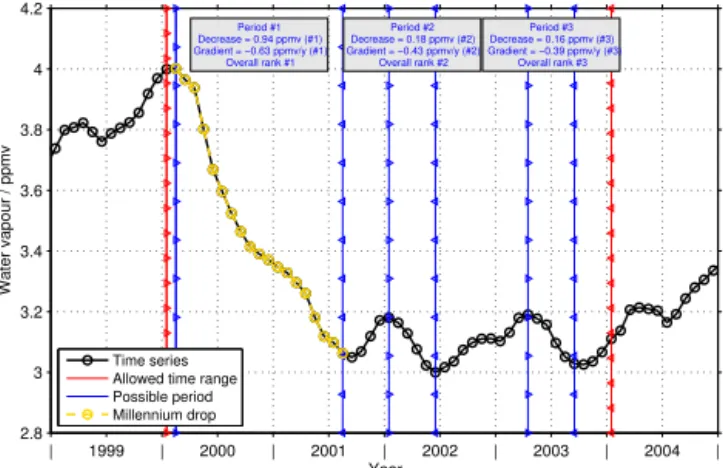
| 1999 | 2000 | 2001 | 2002 | 2003 | 2004 | 2.8
3 3.2 3.4 3.6 3.8 4 4.2
Period #1 Decrease = 0.94 ppmv (#1) Gradient = −0.63 ppmv/y (#1)
Overall rank #1
Period #2 Decrease = 0.18 ppmv (#2) Gradient = −0.43 ppmv/y (#2)
Overall rank #2
Period #3 Decrease = 0.16 ppmv (#3) Gradient = −0.39 ppmv/y (#3)
Overall rank #3
Year
Water vapour / ppmv
Time series Allowed time range Possible period Millennium drop
Figure A1.An example of the millennium drop (phase 1) char-acteristics analysis considering the HALOE/MIPAS time series at 100 hPa at the Equator. The time series is given in black and rep-resents a running mean over 1 year. The red lines indicate the gen-eral time interval where a water vapour decline will be considered. Within this period three periods can be found where water vapour is decreasing. The first period from February 2000 to August 2001 (overplotted in yellow) exhibits both the largest decrease and abso-lute gradient and is therefore selected as the representative period for the millennium drop (phase 1).
can be found in Eichinger et al. (2015) or Schieferdecker et al. (2015).
A4 Analysis approach
The basic data for the analysis presented in Fig. 3 are monthly zonal mean data covering the time period from July 1998 to December 2005. The HALOE-MIPAS data set is interpolated in time to fill a few gaps. The data are aver-aged over a latitude range of 20◦ using a 10◦latitude grid.
The rather wide average in latitude aims to handle some of the sparseness of the HALOE observations. For the simula-tions this would not be necessary but for reasons of compati-bility and comparacompati-bility the same handling is applied. In the vertical the data sets extend from 100 to about 7 hPa and are interpolated on a regular grid using 16 levels per pressure decade.
The analysis is performed separately for every pressure level and latitude bin using the steps listed below. Figure A1 shows an example.
In a first step we calculate a running average over 1 year. In Fig. A1 the averaged time series is given by the black line. Based on that time series, in the next step we calculate the gradient in water vapour along every data point.
from January 2000 to January 2004, as indicated by the red lines in Fig. A1. This is based on a priori knowledge. For higher altitudes we adjust the start of the interval to the start date of the millennium drop at 100 hPa. At this altitude the drop is typically easiest to observe and we expect that higher up no earlier start dates occur.
To decide which of the periods represents the millennium drop, we rely on two parameters: one, the absolute change in water vapour and, two, its overall gradient. These parameters are calculated for every period. Subsequently the periods are ranked according to these parameters with the largest abso-lute value gaining the highest rank. The ranks for a period are summed up and the period with the lowest sum is consid-ered as the period that most likely represents the millennium drop. In the example shown in Fig. A1 the first period is cho-sen to reprecho-sent the millennium drop as it exhibits both the largest decrease and the strongest negative gradient among the possible periods.
Appendix B: Pearson’s correlation coefficient
Pearson’s correlation coefficient is determined by the follow-ing:
r=
Pn
i=1(ai−a)(bi−b)
q
Pn
i=1(ai−a)2 q
Pn
i=1(bi−b)2
, (B1)
whereaandbare the data sets to be correlated.nis the num-ber of values per data set anda=1nPn
The Supplement related to this article is available online at doi:10.5194/acp-16-8125-2016-supplement.
Author contributions. Sabine Brinkop prepared the manuscript and analysed the model results. Martin Dameris was involved in the dis-cussion of the data analysis results and supported the writing of the manuscript. Hella Garny calculated the residual circulation based on the model simulations. Patrick Jöckel performed the simulations with EMAC. Gabriele Stiller provided the MIPAS data and partici-pated in the discussion. Stefan Lossow performed the novel analysis of the water vapour drop characteristics with the HALOE/MIPAS and the model simulation data.
Acknowledgements. This work has been funded by the Deutsche Forschungsgemeinschaft (DFG) within the research unit Strato-spheric Change and its Role for Climate Prediction (SHARP-FOR 1095). The presented investigations were carried out within the water vapour project SHARP-WV. The model simulations were performed within the DKRZ project ESCiMo (Earth System Chem-istry integrated Modelling). The merged data set of stratospheric water vapour was kindly provided by M. Hegglin. We would like to thank the Deutsches Klimarechenzentrum (DKRZ) for providing computing time and support and Christoph Kiemle for valuable comments on the manuscript. We thank S. Fueglistaler, M. Schoeberl and an anonymous referee for valuable comments on the manuscript.
The article processing charges for this open-access publication were covered by a Research
Centre of the Helmholtz Association.
Edited by: P. Haynes
References
Calvo, N., Garcia, R. R., Randel, W. J., and Marsh, D. R.: Dynami-cal mechanism for the increase in tropiDynami-cal upwelling in the lower-most tropical stratosphere during warm ENSO events, J. Atmos. Sci., 67, 2331–2340, 2010.
Deckert, R. and Dameris, M.: Higher tropical SSTs strengthen the tropical upwelling via deep convection, Geophys. Res. Lett., 35, L10813, doi:10.1029/2008GL033719, 2008.
Dessler, A. E., Schoeberl, M. R., Wang, T., Davis, S. M., Rosenlof, K. H., and Vernier, J.-P.: Variations of stratospheric water vapor over the past three decades, J. Geophys. Res., 119, 12588–12598, doi:10.1002/2014JD021712, 2014.
Eichinger, R., Jöckel, P., and Lossow, S.: Simulation of the isotopic composition of stratospheric water vapour – Part 2: Investigation
of HDO/H2O variations, Atmos. Chem. Phys., 15, 7003–7015,
doi:10.5194/acp-15-7003-2015, 2015
Eyring, V. and Lamarque, J.-F.: Global chemistry-climate mod-eling and evaluation, EOS T. Am. Geophys. Un., 93, 539, doi:10.1029/2012EO510012, 2012.
Fischer, H., Birk, M., Blom, C., Carli, B., Carlotti, M., von Clar-mann, T., Delbouille, L., Dudhia, A., Ehhalt, D., EndeClar-mann, M., Flaud, J. M., Gessner, R., Kleinert, A., Koopman, R., Langen, J., López-Puertas, M., Mosner, P., Nett, H., Oelhaf, H., Perron, G., Remedios, J., Ridolfi, M., Stiller, G., and Zander, R.: MIPAS: an instrument for atmospheric and climate research, Atmos. Chem. Phys., 8, 2151–2188, doi:10.5194/acp-8-2151-2008, 2008. Fueglistaler, S. and Haynes, P. H.: Control of interannual and
longer-term variability of stratospheric water vapor, J. Geophys. Res., 110, D24108, doi:10.1029/2005JD006019, 2005.
Fueglistaler, S., Bonazzola, M., Haynes, P., and Peter, T.: Strato-spheric water vapor predicted from the Lagrangian temperature history of air entering the stratosphere in the tropics, J. Geophys. Res., 110, D08107, doi:10.1029/2004JD005516, 2005.
Fueglistaler, S., Liu, Y. S., Flannaghan, T. J., Haynes, P. H., Dee, D. P., Read, W. J., Remsberg, E. E., Thomason, L. W., Hurst, D. F., Lanzante, J. R., and Bernath, P. F.: The re-lation between atmospheric humidity and temperature trends for stratospheric water, J. Geophys. Res., 118, 1052–1074, doi:10.1002/jgrd.50157, 2013.
Garfinkel, C. I., Hurwitz, M. M., Oman, L. D., and Waugh, D. W.: Contrasting Effects of Central Pacific and Eastern Pacific El Niño on Water Vapor, Geophys. Res. Lett., 40, 4115–4120, doi:10.1002/grl.50677, 2013a.
Garfinkel, C. I., Waugh, D. W., Oman, L. D., Wang, L., and Hur-witz, M. M.: Tem- perature trends in the tropical upper tropo-sphere and lower stratotropo-sphere: connections with sea surface tem-peratures and implications for water vapor and ozone, J. Geo-phys. Res.-Atmos., 118, 9658–9672, doi:10.1002/jgrd.50772, 2013b.
Gettelman, A., Birner, T., Eyring, V., Akiyoshi, H., Bekki, S., Brühl, C., Dameris, M., Kinnison, D. E., Lefevre, F., Lott, F., Mancini, E., Pitari, G., Plummer, D. A., Rozanov, E., Shi-bata, K., Stenke, A., Struthers, H., and Tian, W.: The Tropical Tropopause Layer 1960–2100, Atmos. Chem. Phys., 9, 1621– 1637, doi:10.5194/acp-9-1621-2009, 2009.
Gettelman, A., Hegglin, M. I., Son, S.-W., Kim, J., Fujiwara, M., Birner, T., Kremser, S., Rex, M., Añel, J. A., Akiyoshi, H., Austin, J., Bekki, S., Braesike, P., Brühl, C., Butchart, N., Chip-perfield, M., Dameris, M., Dhomse, S., Garny, H., Hardiman, S. C., Jöckel, P., Kinnison, D. E., Lamarque, J. F., Mancini, E., Marchand, M., Michou, M., Morgenstern, O., Pawson, S., Pitari, G., Plummer, D., Pyle, J. A., Rozanov, E., Scinocca, J., Shepherd, T. G., Shibata, K., Smale, D., Teyssèdre, H., Tian, W.: Multimodel assessment of the upper troposphere and lower stratosphere: Tropics and global trends, J. Geophys. Res., 115, D00M08, doi:10.1029/2009JD013638, 2010.
Giorgetta, M. A., Manzini, E., and Roeckner, E.: Forc-ing of the quasi-biennial oscillation from a broad spec-trum of atmospheric waves, Geophys. Res. Lett., 29, 86.1– 86.4,doi:10.1029/2002GL014756, 2002.
S. K., Boschung, J., Nauels, A., Xia, Y., Bex, V., and Midgley, P. M., Cambridge University Press, Cambridge, UK, and New York, NY, USA, 2013.
Hegglin, M. I., Tegtmeier, S., Anderson, J., Froidevaux, L., Fuller, R., Funke, B., Jones, A., Lingenfelser, G., Lumpe, J., Pendlebury, D., Remsberg, E., Rozanov, A., Toohey, M., Ur-ban, J., von Clarmann, T., Walker, K. A., Wang, R., and Weigel, K.: SPARC Data Initiative: Comparison of water vapor climatologies from international satellite limb sounders, J. Geo-phys. Res.-Atmos., 118, 11824–11846, doi:10.1002/jgrd.50752, 2013.
Hegglin, M. I., Plummer, D. A., Shepherd, T. G., Scinocca, J. F., Anderson, J., Froidevaux, L., Funke, B., Hurst, D., Rozanov, A., Urban, J., von Clarmann, T., Walker, K. A., Wang, H. J., Tegt-meier, S., and Weigel, K.: Vertical structure of stratospheric water vapour trends derived from merged satellite data, Nat. Geosci., 7, 768–776, 2014.
Holton, J. R.: An Introduction to Dynamic Meteorology, Interna-tional Geophysics Series, 4th Edn., Academic Press, San Diego, New York, USA, 2004.
Hurst, D. F., Oltmans, S. J., Vömel, H., Rosenlof, K. H., Davis, S. M., Ray, E. A., Hall, E. G., and Jordan, A. F.: Strato-spheric water vapor trends over Boulder, Colorado: analysis of the 30 year boulder record, J. Geophys. Res., 116, D02306, doi:10.1029/2010JD015065, 2011.
Jöckel, P., Kerkweg, A., Pozzer, A., Sander, R., Tost, H., Riede, H., Baumgaertner, A., Gromov, S., and Kern, B.: Development cycle 2 of the Modular Earth Submodel System (MESSy2), Geosci. Model Dev., 3, 717–752, doi:10.5194/gmd-3-717-2010, 2010. Jöckel, P., Tost, H., Pozzer, A., Kunze, M., Kirner, O.,
Brenninkmei-jer, C. A. M., Brinkop, S., Cai, D. S., Dyroff, C., Eckstein, J., Frank, F., Garny, H., Gottschaldt, K.-D., Graf, P., Grewe, V., Kerkweg, A., Kern, B., Matthes, S., Mertens, M., Meul, S., Neu-maier, M., Nützel, M., Oberländer-Hayn, S., Ruhnke, R., Runde, T., Sander, R., Scharffe, D., and Zahn, A.: Earth System Chem-istry integrated Modelling (ESCiMo) with the Modular Earth Submodel System (MESSy) version 2.51, Geosci. Model Dev., 9, 1153–1200, doi:10.5194/gmd-9-1153-2016, 2016.
Jones, C. D., Hughes, J. K., Bellouin, N., Hardiman, S. C., Jones, G. S., Knight, J., Liddicoat, S., O’Connor, F. M., Andres, R. J., Bell, C., Boo, K.-O., Bozzo, A., Butchart, N., Cadule, P., Corbin, K. D., Doutriaux-Boucher, M., Friedlingstein, P., Gor-nall, J., Gray, L., Halloran, P. R., Hurtt, G., Ingram, W. J., Lamar-que, J.-F., Law, R. M., Meinshausen, M., Osprey, S., Palin, E. J., Parsons Chini, L., Raddatz, T., Sanderson, M. G., Sellar, A. A., Schurer, A., Valdes, P., Wood, N., Woodward, S., Yoshioka, M., and Zerroukat, M.: The HadGEM2-ES implementation of CMIP5 centennial simulations, Geosci. Model Dev., 4, 543–570, doi:10.5194/gmd-4-543-2011, 2011.
Kley, D., Russell, J. M., and Philips, C.: Stratospheric Processes and their Role in Climate (SPARC) – Assessment of Upper Tro-pospheric and Stratospheric Water Vapour, SPARC Report 2, WMO/ICSU/IOC World Climate Research Programme, Geneva, Switzerland, 2000.
Löffler, M., Brinkop, S., and Jöckel, P.: Impact of major volcanic eruptions on stratospheric water vapour, Atmos. Chem. Phys., 16, 6547–6562, doi:10.5194/acp-16-6547-2016, 2016.
Maycock, A. C., Joshi, M. M., Shine, K. P., Davis, S. M., and Rosenlof, K. H.: The potential impact of changes in lower
stratospheric water vapour on stratospheric temperatures over the past 30 years, Q. J. Roy. Meteor. Soc., 140, 2176–2185, doi:10.1002/qj.2287, 2014.
Mote, P. W., Rosenlof, K. H., Holton, J. R., Harwood, R. S., and Wa-ters, J. W.: An atmospheric tape recorder: the imprint of tropical tropopause temperatures on stratospheric water vapor, J. Geo-phys. Res., 101, 3989–4006, 1996.
Randel, W. J. and Jensen, E. J.: Physical processes in the tropi-cal tropopause layer and their roles in a changing climate, Nat. Geosci., 6, 169–176, doi:10.1038/ngeo1733, 2013.
Randel, W. J., Wu, F., Oltmans, S. J., Rosenlof, K., and Nedoluha, G.: Interannual changes of stratospheric water vapor and correlations with tropical tropopause temperatures, J. Atmos. Sci., 61, 2133–2148, 2004.
Randel, W. J., Wu, F., Vömel, H., Nedoluha, G. E., and Forster, P.: Decreases in stratospheric water vapor after 2001: links to changes in the tropical tropopause and the Brewer–Dobson circulation, J. Geophys. Res., 111, D12312, doi:10.1029/2005JD006744, 2006.
Randel, W. J., Garcia, R. R., Calvo, N., and Marsh, D.: ENSO influence on zonal mean temperature and ozone in the trop-ical lower stratosphere, Geophys. Res. Lett., 36, L15822, doi:10.1029/2009GL039343, 2009.
Roeckner, E., Brokopf, R., Esch, M., Giorgetta, M., Hagemann, S., Kornblueh, L., Manzini, E., Schlese, U., and Schulzweida, U.: Sensitivity of simulated climate to horizontal and vertical reso-lution in the ECHAM5 atmosphere model, J. Climate, 19, 3771– 3791, doi:10.1175/JCLI3824.1, 2006.
Rosenlof, K. H. and Reid, G. C.: Trends in the tempera-ture and water vapor content of the tropical lower strato-sphere: sea surface connection, J. Geophys. Res., 113, D06107, doi:10.1029/2007JD009109, 2008.
Russell, J. M., Gordley, L. L., Park, J. H., Drayson, S. R., Hes-keth, W. D., Cicerone, R. J., Tuck, A. F., Frederick, J. E., Har-ries, J. E., and Crutzen, P. J.: The halogen occultation experi-ment, J. Geophys. Res., 98, 10777–10797, 1993.
Scaife, A. A., Butchart, N., Jackson, D.R., and Swinbank, R.: Can changes in ENSO activity help to explain increasing stratospheric water vapor?, Geophys. Res. Lett., 30, 1880, doi:10.1029/2003GL017591, 2003.
Scherer, M., Vömel, H., Fueglistaler, S., Oltmans, S. J., and Staehe-lin, J.: Trends and variability of midlatitude stratospheric water vapour deduced from the re-evaluated Boulder balloon series and HALOE, Atmos. Chem. Phys., 8, 1391–1402, doi:10.5194/acp-8-1391-2008, 2008.
Schieferdecker, T.: Variabilität von Wasserdampf in der unteren und mittleren Stratosphäre auf der Basis von HALOE/UARS und MIPAS/Envisat Beobachtungen, PhD thesis, Karlsruhe Institute oft Technology, available at: http://digbib.ubka.uni-karlsruhe.de/ volltexte/1000046296, last access: 22 June 2015.
Schieferdecker, T., Lossow, S., Stiller, G. P., and von Clarmann, T.: Is there a solar signal in lower stratospheric water vapour?, Atmos. Chem. Phys., 15, 9851–9863, doi:10.5194/acp-15-9851-2015, 2015.
Schoeberl, M. R., Dessler, A. E., and Wang, T.: Simulation of strato-spheric water vapor and trends using three reanalyses, Atmos. Chem. Phys., 12, 6475–6487, doi:10.5194/acp-12-6475-2012, 2012.
Solomon, S., Rosenlof, K. H., Portmann, R. W., Daniel, J. S., Davis, S. M., Sanford, T. S., and Plattner, G.-K.: Con-tributions of stratospheric water vapor to decadal changes in the rate of global warming, Science, 327, 1219–1223, doi:10.1126/science.1182488, 2010.
SPARC CCMVal (Stratospheric Processes And their Role in Climate): SPARC Report on the Evaluation of Chemistry-Climate Models, edited by: Eyring, V., Shepherd, T. G., and Waugh, D. W., SPARC Report No. 5, WCRP-132, WMO/TD-No. 1526, 478 pp., available at: http://www.atmosp.physics. utoronto.ca/SPARC/ccmval_final/index.php (last access: 22 June 2015), 2010.
Stenke, A. and Grewe, V.: Simulation of stratospheric water vapor trends: impact on stratospheric ozone chemistry, Atmos. Chem. Phys., 5, 1257–1272, doi:10.5194/acp-5-1257-2005, 2005. Urban, J., Lossow, S., Stiller, G., and Read, W.: Another drop in
water vapor, EOS, 95, 245–246, 2014.