www.nonlin-processes-geophys.net/23/159/2016/ doi:10.5194/npg-23-159-2016
© Author(s) 2016. CC Attribution 3.0 License.
Detecting and tracking eddies in oceanic flow fields: a Lagrangian
descriptor based on the modulus of vorticity
Rahel Vortmeyer-Kley1, Ulf Gräwe2,3, and Ulrike Feudel1
1Institute for Chemistry and Biology of the Marine Environment, Theoretical Physics/Complex Systems, Carl von Ossietzky University Oldenburg, Oldenburg, Germany
2Leibniz Institute for Baltic Sea Research, Rostock-Warnemünde, Germany
3Institute of Meteorology and Climatology, Leibniz Universität Hannover, Hanover, Germany
Correspondence to:Rahel Vortmeyer-Kley ([email protected])
Received: 29 January 2016 – Published in Nonlin. Processes Geophys. Discuss.: 10 February 2016 Revised: 19 May 2016 – Accepted: 2 June 2016 – Published: 5 July 2016
Abstract.Since eddies play a major role in the dynamics of oceanic flows, it is of great interest to detect them and gain in-formation about their tracks, their lifetimes and their shapes. We present a Lagrangian descriptor based on the modulus of vorticity to construct an eddy tracking tool. In our approach we denote an eddy as a rotating region in the flow possess-ing an eddy core correspondpossess-ing to a local maximum of the Lagrangian descriptor and enclosed by pieces of manifolds of distinguished hyperbolic trajectories (eddy boundary). We test the performance of the eddy tracking tool based on this Lagrangian descriptor using an convection flow of four ed-dies, a synthetic vortex street and a velocity field of the west-ern Baltic Sea. The results for eddy lifetime and eddy shape are compared to the results obtained with the Okubo–Weiss parameter, the modulus of vorticity and an eddy tracking tool used in oceanography. We show that the vorticity-based La-grangian descriptor estimates lifetimes closer to the analyt-ical results than any other method. Furthermore we demon-strate that eddy tracking based on this descriptor is robust with respect to certain types of noise, which makes it a suit-able method for eddy detection in velocity fields obtained from observation.
1 Introduction
Transport of particles and chemical substances mediated by hydrodynamic flows are important components in the dy-namics of ocean and atmosphere. For this reason, there is an increasing interest in identifying particular structures in
the flows such as eddies or transport barriers to understand their role in transport and mixing of the fluid as well as their impact on marine biology for instance. Of particular inter-est in oceanography are eddies, which can be responsible for the confinement of plankton within them and, hence, im-portant for the development of plankton blooms (Abraham, 1998; Martin et al., 2002; Sandulescu et al., 2007). Such ed-dies possess a large variety of sizes and lifetimes. To tackle the problem of recognizing such eddies in aperiodic flows, different approaches have been developed: on the one hand, there are several methods available which are inspired by dy-namical systems theory (Haller (2015), Mancho et al. (2013) and references therein); on the other hand, numerical soft-ware for automated eddy detection has been developed in oceanography based on either physical quantities of the flow (Okubo, 1970; Weiss, 1991; Nencioli et al., 2010) or geomet-ric measures (Sadarjoen and Post, 2000).
increas-ing number of eddy-resolvincreas-ing datasets available provided ei-ther by observations (Donlon et al., 2012) or by numerical simulations (Thacker et al., 2004; Dong et al., 2009). Con-sequently there is a growing interest in the census of eddies, their size and lifetimes depending on the season. This task re-quires robust algorithms for the computation of eddy bound-aries as well as the precise detection of their appearance and disappearance in time based on numerical velocity fields (Pe-tersen et al., 2013; Wischgoll and Scheuermann, 2001; Dong et al., 2014) as well as altimetry data (Chaigneau et al., 2008; Chelton et al., 2011). However, the huge amount of avail-able data poses a challenge to data analysis. As pointed out in Chaigneau et al. (2008), mesoscale and submesoscale ed-dies cannot be extracted from a turbulent flow without a suit-able definition and a competitive automatic identification al-gorithm. Several such algorithms have been developed based on the various concepts mentioned above. In the following we will briefly discuss several of those algorithms.
Based on dynamical systems theory, one can search for Lagrangian coherent structures (LCSs) which describe the most repelling or attracting manifolds in a flow (Haller and Yuan, 2000). The time evolution of these invariant mani-folds makes up the Lagrangian skeleton for the transport of particles in fluid flows. LCSs can be considered as the organizing centres of hydrodynamic flows. Their computa-tion is based on the search for stacomputa-tionary curves of shear in the case of hyperbolic or parabolic LCSs. Elliptic LCSs like eddies are computed as stationary curves of averaged strain (Haller and Beron-Vera, 2013; Karrasch et al., 2015; Onu et al., 2015) or Lagrangian-averaged vorticity deviation (Haller et al., 2016). Other methods to determine whether an eddy can be identified in the flow employ average Lagrangian velocities (Mezi´c et al., 2010) or burning invariant manifolds (Mitchell and Mahoney, 2012). The latter were originally in-troduced to track fronts in reaction diffusion systems (Ma-honey et al., 2012) but have recently been extended to the detection of eddies (Mahoney and Mitchell, 2015). A com-pletely different approach which connects geometric prop-erties of a flow with probabilistic measures utilizes transfer operators to identify LCSs (Froyland and Padberg, 2009). Another approach is the computation of distinguished hyper-bolic trajectories (DHTs) and their stable and unstable man-ifolds to identify Lagrangian coherent structures in a flow. DHTs can be considered as a generalization of stagnation points of saddle type and their separatrices to general time-dependent flows (Ide et al., 2002; Wiggins, 2005; Mancho et al., 2006). DHTs and their manifolds can be computed us-ing Lagrangian descriptors, which integrate intrinsic physical properties for a finite time and thereby reveal the geometric structures in phase space (Mancho et al., 2013). Stable and unstable manifolds can also be calculated using the ridges of finite-time or finite-size Lyapunov exponents (FTLEs or FSLEs) (Artale et al., 1997; Boffetta et al., 2001; d’Ovidio et al., 2004; Branicki and Wiggins, 2010) using the idea that initially nearby particles in a flow will move apart in
stretch-ing regions, while they will move closer to each other in con-tracting regions.
Despite the discussion about objectivity (cf. Haller’s short comment SC2 in the discussion of this paper, Mancho’s ed-itor comment EC1 and Mendoza and Mancho, 2012) the method of Lagrangian descriptors is very appealing and is appropriate to gain insight into oceanographic flows. It has already been successfully applied to compute Lagrangian co-herent structures in the Kuroshio current (Mendoza et al., 2010; Mendoza and Mancho, 2010, 2012), in the polar vortex (de la Cámara et al., 2012), in the north-western Mediter-ranean Sea (Branicki et al., 2011) and for analysing the possible dispersion of debris from the Malaysian Airlines flight MH370 airplane in the Indian Ocean (García-Garrido et al., 2015).
In the recent years there has been some effort to derive Eulerian quantities which can be used to draw conclusions about Lagrangian transport phenomena (Sturman and Wig-gins, 2009; McIlhany and WigWig-gins, 2012; McIlhany et al., 2011, 2015).
In oceanography, one of the most popular methods with which to identify eddies is based on the Okubo–Weiss pa-rameter (Okubo, 1970; Weiss, 1991). This method relies on the strain and vorticity of the velocity field and has been ap-plied to both numerical ocean model output and satellite data (Isern-Fontanet et al., 2006; Chelton et al., 2011). Often, the underlying velocity field is derived from altimetric data un-der the assumption of geostrophic theory. In this approach two limitations can appear. First, the derivation of the veloc-ity field can induce noise in the strain and vorticveloc-ity field. This is usually reduced by applying a smoothing algorithm, which might, in turn, remove physical information. Secondly, Dou-glass and Richman (2015) show that eddies can have a sig-nificant ageostrophic contribution. Thus, the detection might fail when relying on geostrophic theory. A slightly different approach was developed by Yang et al. (2001) and Fernandes et al. (2011), who used the signature of eddies in the sea sur-face temperature (SST) to detect them. The partially sparse coverage of satellite SST data limits the application of this method.
a unique way. Moreover, the relative velocity in the eddy core should vanish and should be enclosed by closed streamlines. This detection and tracking algorithm was successfully ap-plied by Dong et al. (2012) in the Southern California Bight. In addition, the detection algorithm of Nencioli et al. (2010) has the advantage that its application is not limited to surface fields (Isern-Fontanet et al., 2006; Chelton et al., 2011; Fer-nandes et al., 2011). Thus, it is possible to track eddies in the interior of the ocean, without any surface signature.
In this paper we develop an eddy detection and tracking tool based on the method of the Lagrangian descriptor in-troduced by Mancho and co-workers (Madrid and Mancho, 2009; Mancho et al., 2013). For the purpose of automated eddy detection we propose to use the modulus of the vortic-ity as the scalar quantvortic-ity to be computed along a trajectory instead of using the arc length of trajectories. We compare our method to four others, namely the original Lagrangian descriptor using the arc length (Madrid and Mancho, 2009; Mendoza et al., 2010), an oceanographic method based on geometric properties of the flow field (Nencioli et al., 2010) and detection tools which employ the Okubo–Weiss parame-ter (Okubo, 1970; Weiss, 1991) and the modulus of vorticity itself.
The paper is organized as follows: Sect. 2 briefly reviews the Eulerian concepts of vorticity and the Okubo–Weiss pa-rameter, as well as the Lagrangian descriptors M based on the arc length andMVbased on the modulus of vorticity. To compare the performance of the two Lagrangian descriptors and the Eulerian concepts, we use two simple velocity fields: the model of four counter-rotating eddies and a modified van Kármán vortex street in Sect. 3. In Sect. 4 we describe the im-plementation of the Lagrangian descriptor based on the mod-ulus of vorticity as a tracking tool identifying eddy lifetimes (Sect. 4.1) and compare the results again with the other afore-mentioned methods. In Sect. 4.2 we study the performance of the method in cases where we corroborate the velocity fields with noise to test the robustness of the method if applied to velocity fields obtained from observational data. Finally in Sect. 4.3 we compare the Eulerian and the Lagrangian view of the eddy shape with application to the modified van Kár-mán vortex street and to a velocity field from oceanography describing the dynamics of the western Baltic Sea (Gräwe et al., 2015a). We conclude the paper with a discussion in Sect. 5.
2 From Eulerian to Lagrangian methods
The dynamics of a fluid can be characterized employing two different concepts: the Eulerian and the Lagrangian view. While the Eulerian view uses quantities describing different properties of the velocity field, the Lagrangian view provides quantities from the perspective of a moving fluid particle. Out of the variety of different Eulerian and Lagrangian meth-ods mentioned in the Introduction, we recall here briefly only
those concepts which will be important for our development of a measure to identify eddies in a flow.
A Eulerian method to describe the circulation density of a velocity field in hydrodynamics is vorticityW(x,t ),
de-fined as the curl of the velocity fieldv(x,t ). The vorticity
associates a vector with each point in the fluid representing the local axis of rotation of a fluid particle. It displays areas with a large circulation density like eddies as regions of large vorticity and eddy cores as local maxima.
Another Eulerian quantity is the Okubo–Weiss parame-ter OW. It weights the strain properties of the flow against the vorticity properties and thus distinguishes strain-dominated areas from the vorticity-dominated one. The Okubo–Weiss parameter is defined as
OW=sn2+ss2−ω2, (1)
where the normal strain componentsn, the shear strain com-ponentss and the relative vorticityω of a two-dimensional velocity fieldv=(u,v) are defined as
sn=
∂u
∂x−
∂v ∂y, ss=
∂v
∂x+
∂u
∂y andω=
∂v
∂x−
∂u
∂y. (2)
Eddies are areas that have a negative Okubo–Weiss param-eter with a local minimum at the eddy core because here the vorticity component outweighs the strain component, while strain-dominated areas are characterized by a positive Okubo–Weiss parameter.
A Lagrangian view of the dynamics of the velocity field is given by the Lagrangian descriptor developed by Mancho and co-workers (Madrid and Mancho, 2009). A more general definition of the Lagrangian descriptor is outlined in Mancho et al. (2013). Here we focus on the Lagrangian descriptor based on the arc length of a trajectory, defined as
M x∗, t∗ v,τ=
t∗+τ Z
t∗−τ n X i=1
dxi(t )
dt
2!1/2
dt, (3)
withx(t )=(x1(t ),x2(t ). . . xn(t )) being the trajectory of a
fluid particle in the velocity fieldvthat is defined in the time
interval [t∗−τ,t∗+τ] and going through the point x∗ at
timet∗.
The Lagrangian descriptorMyields singular features that can be interpreted as time-dependent “phase space struc-tures” like (time-dependent or moving) elliptic or hyperbolic “fixed” points (denoted as distinguished elliptic or hyper-bolic trajectories, DET and DHT respectively, in Madrid and Mancho, 2009) and their time-dependent stable and unsta-ble manifolds (Mancho et al., 2013; Wiggins and Mancho, 2014). The reason for the singular features ofM is thatM
the case for DHTs and their stable and unstable manifolds. Trajectories on both sides of the manifold have a different behaviour compared to the behaviour of the trajectories on the manifold. Either they approach the manifold very fast or they move away from the manifold very fast. In both cases they accumulate larger values ofMin a given time interval than trajectories on the manifold. Therefore, the singular line ofMin a colour-coded plot ofMcan be interpreted as cor-responding to a manifold. If a trajectory stays in a region or at one point, it accumulates a small or zero value ofMand
Mbecomes a local minimum. While DHTs have been exten-sively studied, distinguished trajectories possessing an ellip-tic type are less understood. However, such trajectories can also be identified as singular features ofMbeing surrounded by an elliptic region in the sense of Mancho et al. (2013). For an extensive discussion about the notion of hyperbolic and elliptic regions in flows we refer to Mancho et al. (2013).
For each instant of timet∗the colour-coded plots ofMcan be interpreted as a “snapshot” of the phase space, where the minima correspond to one point of a DHT or a distinguished trajectory surrounded by an elliptic region. Whent∗changes,
Mreveals the time evolution of the phase space and, loosely speaking, distinguished hyperbolic trajectories can be con-sidered as “moving saddle points”, and distinguished trajec-tories surrounded by an elliptic region in the sense of Man-cho et al. (2013) as “moving elliptic points”. Due to the ar-bitrary time dependence of the flow, both the DHTs and the distinguished trajectories surrounded by an elliptic region are time-dependent and exist in general only for a finite time in a time-dependent flow. Hyperbolicity in the case of DHT refers to the fact that along those trajectories Lyapunov exponents are positive or negative but not zero except for the direction along the trajectory (Mancho et al., 2013).
Because the Lagrangian descriptorMwould display min-ima in both cases, i.e. DHT and distinguished trajectories sur-rounded by an elliptic region, a second criterion is needed to distinguish them properly. To avoid such an additional dis-tinction criterion, we suggest a Lagrangian descriptor based on the modulus of vorticity to simplify the automated eddy detection. We emphasize that it has already been pointed out by Mancho et al. (2013) that any intrinsic physical or geo-metrical property of trajectories can be used to construct a Lagrangian descriptor by integrating this property along tra-jectories over a certain time interval. Therefore, we intro-duce a vorticity-based Lagrangian descriptor MV in which the physical quantity is the modulus of the vorticityW of a velocity fieldv(x,t ):
W (x, t )= |∇ ×v(x, t )|. (4)
We define the Lagrangian descriptorMVbased on the mod-ulus of vorticity as
MV x∗, t∗
τ=
t∗+τ Z
t∗−τ
(W (x, t ))1/2dt. (5)
The Lagrangian descriptorMVbased on the modulus of vor-ticity measures the Eulerian quantity modulus of vorvor-ticity along a trajectory (Lagrangian view) passing through a po-sitionx∗at timet∗in a time interval [t∗−τ,t∗+τ]. Within
this time interval trajectories accumulate different values ofMV. Similar to the arc-length-based Lagrangian descrip-torM, the Lagrangian descriptorMVbased on the modulus of vorticity displays singular features such as lines or local minima or maxima. in the case of local maxima, a trajec-tory does not leave the region of large values of the mod-ulus of vorticity. Such regions are typical for the inner part of an eddy. Therefore, a local maximum corresponds to the eddy core and can be interpreted as a snapshot of the distin-guished trajectory at timet∗surrounded by an elliptic region in the sense of Mancho et al. (2013). By contrast, local min-ima ofMVarise if a trajectory stays in a region of small val-ues of the modulus of vorticity. In analogy with the singular lines in the case ofM, singular lines of MV can be inter-preted as the boundaries of regions of different dynamical behaviour. In this sense they can be understood as manifolds of the DHTs.
The local maxima and the singular lines of MV will be used to construct an eddy tracking tool based on the follow-ing concept of an eddy: we denote an eddy as befollow-ing bounded by pieces of stable and unstable manifolds of DHTs (accord-ing to Branicki et al., 2011, and Mendoza and Mancho, 2012) surrounding an area in which the flow is rotating. The man-ifolds correspond to singular lines inMV which are used to describe the eddy boundaries. The eddy core is considered to be a local maximum ofMVwithin this bounded region and can be interpreted as one point of a distinguished trajectory surrounded by an elliptic region.
In the case ofMVas well as in the case ofMthe resolu-tion of these structures depends on the choice of the param-eter τ that gives the length of the time interval. Structures that live shorter than 2τ cannot be resolved. Even structures that live longer than 2τ can only be resolved ifτ is chosen large enough. The choice ofτ depends on the structure and the timescale of the flow field considered. Within the range of the timescale of the problem that should be resolved some variation ofτ is needed until the optimalτ for a given prob-lem is found.
3 Eddies in a flow: comparing Eulerian and Lagrangian methods
(a)
0 0.5 1
x
1
0.5
0
y
(b)
0 0.5 1
x
0 0.2 0.4 0.6 0.8 1
Figure 1. Colour-coded representation of the modulus of vortic-ity (a)and the Okubo–Weiss parameter (b)for the eddy field in Eq. (6). All plots are normalized to the maximum value.
(a)1
0.5
0
y
(b) (c)
(d)
0 0.5 1
x
1
0.5
0
y
(e)
0 0.5 1
x
(f)
0 0.5 1
x
0 0.1 0.2 0.3 0.4 0.5 0.6 0.7 0.8 0.9 1
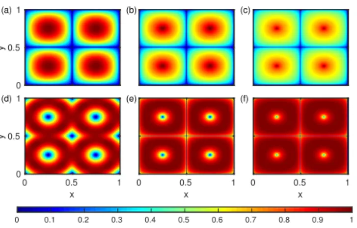
Figure 2.Colour-coded representation of the Lagrangian descriptor
MV(a)–(c)and the Lagrangian descriptorM (d)–(f)for the eddy
field in Eq. (6) withτchosen as 0.5(a, d), 25(b, e)and 100(c, f). All plots are normalized to the maximum value.
The four counter-rotating eddies are employed to show that different methods detect different aspects of the eddies. Ad-ditionally, we discuss how the displayed structure depends on the chosenτ. The vortex street is particularly used to test how suitable our method is to detecting and tracking eddies in comparison to other methods and how well they all esti-mate eddy lifetimes and shapes. This way we gain insight into performance, advantages and disadvantages of the pro-posed method compared to the others.
To give a complete view of the advantages and disadvan-tages, the results of the different test cases are interpreted in a coherent discussion after presenting all results.
The equations of motion of fluid particles in a convection flow of four counter-rotating eddies are given by
u= ˙x=sin(2π·x)·cos(2π·y)
v= ˙y= −cos(2π·x)·sin(2π·y). (6)
We compute the four different quantities, the modulus of vor-ticity, the Okubo–Weiss parameter and the two Lagrangian descriptors M and MV in a spatial domain [0, 1]×[0, 1]. To this end, the spatial domain is decomposed into a discrete grid (201×201), and the different methods are calculated for each grid point. The results are presented in Figs. 1 and 2.
(d)
-5 -4 -2 0 2 4 6 8 10 x
(c) (a)3
2 1 0 -1 -2 -3
y
(b)
-5 -4 -2 0 2 4 6 8 10 x
3 2 1 0 -1 -2 -3
y
Figure 3.Modulus of vorticity(a), Okubo–Weiss parameter(b), Lagrangian descriptorM (c) and Lagrangian descriptor MV (d)
for the hydrodynamic model of a vortex street att=0.151 with
τ=0.15, normalized to the maximum value. Blue colours indicate small values, and red large values of the depicted quantity. The dark blue regions in(c)and(d)are regions where the trajectories have left the region of interest.
The model of the vortex street consists of two eddies that emerge at two given positions in space, travel a distanceLin positivexdirection and fade out. The two eddies are counter-rotating. They emerge and die out periodically with a time shift of half a period. The model is adapted from Jung et al. (1993) and Sandulescu et al. (2006), with the difference that the cylinder as the cause of eddy formation and its impact on the flow field due to its shade are neglected. In this sense, the eddies emerge non-physically out of nowhere, but all quanti-ties like lifetime and radius to be estimated by means of eddy tracking are then given analytically and make up a perfect test scenario. A detailed description of the model can be found in the Supplement to this article. Again all methods are applied to this velocity field using a (302×122) grid. Unless other-wise stated, the time intervalτ for the Lagrangian methods is set to 0.15 times the lifetime of an eddy. The results are presented in Fig. 3.
To characterize Lagrangian coherent structures in a flow, not only do distinguished trajectories surrounded by an el-liptic region in the sense of Mancho et al. (2013) associated with eddy cores and DHTs have to be identified; the stable and unstable manifolds associated with the latter have to be identified as well to find eddy boundaries according to the concept of an eddy in Sect. 2. Those manifolds are visible as singular lines in the colour-coded plot of the Lagrangian de-scriptorM(Figs. 2d–f and 3c) and the Lagrangian descriptor
MV(Figs. 2a–c and 3d).
How detailed the displayed fine structure of the La-grangian descriptors M andMV is represented depends on the chosen value of the time interval τ. It ranges from no clear structure for smallτ (Fig. 2a and d) to a detailed struc-ture for largeτ (Fig. 2c and f).
From these properties, distinction between DHTs and eddy cores and identification of manifolds, we can conclude that the Lagrangian descriptorMV is a suitable method for an automated search for eddies in oceanographic flows. Out of the four considered quantities,MVbest allows for a clear identification of eddy cores and the stable and unstable man-ifolds of DHTs necessary to get more insight into the size of eddies with the least smallest number of check criteria. For this reason we suggest using MV as the basis for an eddy tracking tool. How these properties ofMVare implemented into an eddy tracking tool is explained for the eddy core in Sect. 4.1 and the eddy size and shape in Sect. 4.3.
4 The Lagrangian descriptorMVas an eddy tracking tool
The mean oceanic flow is superimposed by many eddies of different sizes which emerge at some time instant, persist for some time interval and disappear. Consequently, an eddy tracking tool has to detect them at the instance of emergence, track them over their lifetime and detect their disappearance. To classify the different eddies, some information about their size is needed too. This way one can finally obtain the time evolution of a size distribution function of eddies.
In this section we apply the modulus-of-vorticity-based Lagrangian descriptorMV to the hydrodynamic model of a vortex street to test its performance as an eddy tracking tool. We use the local maxima ofMVfor an automated search for eddy cores and, in addition, the area enclosed by the singular lines ofMVassociated with the manifolds of the DHTs as a measure of the size of the eddies.
4.1 Eddy birth and lifetime
First we check how well MV detects the birth of an eddy and its lifetime and compare the results to the oceanographic eddy tracking tool box (ETTB) by Nencioli et al. (2010), as well as Eulerian quantities like the Okubo–Weiss parameter and the modulus of vorticity.
0.2 0.3 0.4 0.5 0.6 0.7 0.8 0.9 1
Lifetime Tc
0 0.1 0.2 0.3 0.4 0.5 0.6 0.7 0.8 0.9 1
Measured lifetime
M
V w50
MV w100
M
V w200
ETTB w50 ETTB w100 ETTB w200 OW w50 OW w100 OW w200 absVorticity w50 absVorticity w100 absVorticity w200 Analytical lifetime
Figure 4.Eddy lifetime estimated with Okubo–Weiss (OW, vio-let); the modulus of vorticity (absVorticity, cyan);MV (red); and the eddy tracking tool box (ETTB, blue) by Nencioli et al. (2010) for vortex strengthw50, 100 and 200. The black diagonal depicts the analytical lifetime.
The idea of the tracking inspired by Nencioli et al. (2010) is to search for local maxima (MVand modulus of vorticity) or local minima (Okubo–Weiss and velocity-based method by Nencioli et al., 2010) surrounded by a region of gradient towards the maximum or minimum in a given search win-dow. The size of the search window determines which maxi-mal eddy size can be detected. The eddy is tracked from one time step to the next by searching for an eddy core with the same direction of rotation within a given distance. The choice of this distance depends on the velocity field. It should be in the range of the maximal distance a particle could travel in the time span of interest. The position of an eddy is logged in a track list for each eddy at each time step. A track list that is shorter than a given threshold number of time steps is deleted to focus on eddies which exist longer than this min-imum time interval. A detailed description of the algorithms can be found in the Supplement to this article.
In order to check the accuracy of the eddy tracking algo-rithm, we use the dimensionless model of the vortex street presented in Sect. 3, since the time instant of birth of the ed-dies and their lifetimes are given analytically. We measure both quantities for different dimensionless lifetimesTc and
dimensionless vortex strengths of 50, 100 and 200 for the eddy that arises at timeTc/2. The rationale behind varying
the vortex strength is to estimate how weak an eddy could be to be still reliably detected by the methods. ForMV,τ was chosen as 0.15·Tc. The results are presented in Figs. 4 and 5.
In all cases independent of the vortex strength, the results obtained withMV are close to the analyticalTc (Fig. 4) or
the analytical time instant of birth (Fig. 5). All other methods underestimateTc and overestimate the time instant of birth.
be-0.1 0.15 0.2 0.25 0.3 0.35 0.4 0.45 0.5
Time of birth
0 0.1 0.2 0.3 0.4 0.5 0.6 0.7 0.8
Measured time of birth
MV w50
MV w100
MV w200
ETTB w50 ETTB w100 ETTB w200 OW w50 OW w100 OW w200 absVorticity w50 absVorticity w100 absVorticity w200 Analytical lifetime
Figure 5.Time of birth of an eddy estimated with Okubo–Weiss (OW, violet); the modulus of vorticity (absVorticity, cyan); MV
(red); and the eddy tracking tool box (ETTB, blue) by Nencioli et al. (2010) for vortex strengthw50, 100 and 200. The black diagonal depicts the analytical time of birth of an eddy.
comes more and more difficult to detect the eddy as its rota-tion speed decreases. The reason for the good estimates pro-vided by MV lies in its construction, which makes use of the history of the eddy (past and future). Hence it can detect eddies earlier than they arise by taking into account the fu-ture or detect them longer than they actually exist by looking into the past.MV is not restricted to the information about the velocity field at one instant of time like the other meth-ods. However, the performance ofMV depends on the cho-sen value ofτ (Fig. 6). Ifτ gets too large in relation toTc,
the estimate of the lifetime deviates from the analytical one because the trajectories contain too much of the history of the eddy. There exists a small range of optimalτ for a cer-tain class of eddies. In our case the range is between about 15 and 18 % of the eddy lifetime. We have chosen 15 % of the eddy lifetime, because largerτ values increase the computa-tional costs forMV, too. The range of the optimalτ depends crucially on the application. Other applications might need a larger or smaller τ or aτ that is a compromise between structures with very different lifetimes. It is also advisable to varyτ to detect different size and lifetime spectra of eddies. 4.2 Robustness of the lifetime detection with respect to
noise
Velocity fields describing ocean flows either have a finite res-olution when obtained by simulations or contain measure-ment noise when retrieved from observational data. For this reason, an eddy tracking method has to be robust with re-spect to fluctuations of the velocity field. Therefore, we ex-plore how the detected eddy lifetime depends on noise added to the velocity data.
0 0.1 0.2 0.3 0.4 0.5
τ value 0.3
0.4 0.5 0.6 0.7 0.8 0.9 1 1.1
Measured lifetime
Measured lifetime Analytical lifetime
Figure 6.Measured lifetime of an eddy obtained by means ofMV
(red line) versus the chosenτ(analytical lifetimeTc=1 (blue line); vortex strength: 200).
To test the influence of noise in a manageable test setup where we know all parameters, e.g. eddy lifetime (here
Tc=1) or vortex strength (herew=200), we use the
veloc-ity componentsu(x,y,t )andv(x,y,t )of the vortex street mentioned in Sect. 3 and add three different types of noise to it mimicking measurement noise that can arise in obser-vations. The result are noisy velocity componentsuN(x,y,
t )andvN(x,y,t )for which we calculate Okubo–Weiss, the modulus of vorticity andMV and then apply the different eddy tracking methods. The noise is realized as white Gaus-sian noise in form of a matrix of normally distributed ran-dom numbers of the grid size for each time step multiplied by a factor that is referred to as noise level or noise strength. The noise level is given dimensionless, because the noise is applied to the dimensionless model of the vortex street pre-sented in Sect. 3.
The different noise types and their motivation are as fol-lows:
1. Type 1: we add white Gaussian noise ξ(x, y, t ) of different noise strength σ between 0.05 and 0.95 to the velocity componentsu(x,y, t ) and v(x, y,t ) of the vortex street. The noise is uncorrelated in space and time. The resulting velocity componentsuN(x,y,
t )=u(x, y,t)+σ·ξu(x,y,t ) andvN(x,y,t )=v(x,
y,t )+σ·ξv(x,y,t )in this case are still periodic but
noisy. This type of noise mimics the effect of computing derivatives of observed velocity fields (e.g. by satellites or high-frequency (HF) radar).
0 0.2 0.4 0.6 0.8 1
Noise level
0 0.2 0.4 0.6 0.8 1
Median lifetime
M
V
ETTB OW Abs Vorticity Analytical lifetime
Figure 7.Measured median lifetime obtained by different methods (Okubo–Weiss (OW, violet), the modulus of vorticity (absVorticity, cyan),MV (red) and the eddy tracking tool box (ETTB, blue) by
Nencioli et al. (2010)) depending on the noise level. The compu-tations have been performed in a velocity field mimicking a vortex street with type 1 noise (1000 noise realizations). The error bars in-dicate the whiskers of the distribution in the box plot (not shown here) corresponding to approximately±2.7σ.
strength of noise depends on the signal-to-noise ratio. If we have a strong current, it is easy to detect this by a satellite, since the signal strength is high. This is the op-posite for slow currents, where the noise level is much higher. Thus, we add white noise that is inversely pro-portional to the current speed. The noisy velocity com-ponents are given asuN(x,y,t )=u(x,y,t )+σ·ξu(x, y, t)/(1+max
x,y(u(x, y, t ))) and vN(x, y, t )=v(x, y, t )+σ·ξv(x,y,t)/(1+max
x,y(v(x,y,t ))).
3. Type 3: we add white Gaussian noiseξ(t )of different noise strength σ between 0.05 and 0.5 to the y com-ponent of the eddy centres’ movement. The equations of the unperturbed velocity field contain a part that de-scribes the movement of the eddy centres (see Supple-ment). The motion of theycomponents of the eddy cen-tres in the unperturbed velocity field (u,v) is given by
y1(t )=y0= −y2(t ), where the index 1 or 2 refers to the two eddies. The movement of the eddy centres in the case of noise is given byy1N(t )=y0+σ·ξ(t )and
y2N(t )= −y0+σ·ξ(t ). This type of noise can be ob-served if the velocity fields have to rely on georefer-encing. For instance, satellite-generated velocity fields have to be mapped on a longitude–latitude grid, since the satellite is moving. During this postprocessing step a shift in the georeference is possible, leading to trans-lational shifts and thus to type 3 noise. However, a high noise level of type 3 is not very likely. If one deals with typical geophysical applications, which have a grid res-olution of the order 1 to 10 km, the georeferencing
er-0 0.2 0.4 0.6 0.8 1
Noise level
0 0.2 0.4 0.6 0.8 1
Median lifetime
M
V
ETTB OW Abs Vorticity Analytical lifetime
Figure 8.Measured median lifetime obtained by different methods (Okubo–Weiss (OW, violet), the modulus of vorticity (absVorticity, cyan),MV(red) and the eddy tracking tool box (ETTB, blue) by
Nencioli et al. (2010)) depending on the noise level. The compu-tations have been performed in a velocity field mimicking a vortex street with type 2 noise (1000 noise realizations). The error bars in-dicate the whiskers of the distribution in the box plot (not shown here) corresponding to approximately±2.7σ.
rors are mostly small compared to the grid cell size. For this reason, the considered noise levels for type 3 noise are smaller than for type 1 and 2.
0 0.1 0.2 0.3 0.4 0.5 Noise level
0 0.2 0.4 0.6 0.8 1
Median lifetime
MV ETTB OW Abs Vorticity Analytical lifetime
Figure 9.Measured median lifetime obtained by different methods (Okubo–Weiss (OW, violet), the modulus of vorticity (absVorticity, cyan),MV (red) and the eddy tracking tool box (ETTB, blue) by
Nencioli et al. (2010)) depending on the noise level. The compu-tations have been performed in a velocity field mimicking a vortex street with type 3 noise (1000 noise realizations). The error bars in-dicate the whiskers of the distribution in the box plot (not shown here) corresponding to approximately±2.7σ.
distribution increases in width (Fig. 7). The reason is that the noise gets so large that it increasingly disturbs the key signal for an eddy core until no distinct eddy core can be identified anymore.
In the case of type 2 noise,MVand the ETTB show a sim-ilar behaviour to the case of type 1 noise. Both yield good results independent of the noise level. This is again due to the smoothing process in the case ofMV. The modulus of vorticity performs even better than MV in the case of small noise levels, but its performance drops below the results of
MV with increasing noise level (Fig. 8). The reason is that the key signal for determining an eddy core using the modu-lus of vorticity is stronger in the case of small noise levels and gets disturbed by the noise with increasing noise level. As expected, the performance of Okubo–Weiss decreases with increasing noise level. In contrast to type 1 noise, Okubo– Weiss can identify eddy cores even in the case of strong noise, because the key signal for an eddy core is less dis-turbed.
In the case of type 3 noise,MV yields an estimate of the lifetime with the largest error (Fig. 9). In this case noisy tra-jectories that start close to each other diverge fast, while the ones with no noise have a similar dynamical evolution. This divergence due to noise leads to a loss of structure in space that can be interpreted as a weakening of the correlation be-tween neighbouring trajectories. This effect is strongest in the case ofMVbecause it integrates over time, and so neigh-bouring trajectories that have similar values ofMVin the case of no noise yield very different values ofMVdue to the diver-gence of the trajectories. As a consequence no clear structure
inMVcan be identified. This effect increases with the noise level.
Also for the other methods noise of type 3 affects strongly the identification of the eddy core because the weakening of the correlation between neighbouring points disturbs the key signal of an eddy core (a local minimum or maximum in a certain domain). The error in estimating the lifetime in-creases with increasing noise level. In all cases the number of outliers in the box plot (not shown here) increases with the noise level.
As a consequence, none of the methods performs in an op-timal way when the noise displaces the eddy cores during their motion. This disadvantage will lead to deviations in the lifetime statistics for eddy tracking based on observational data. However, the error in georeferencing of satellite images (which is mimicked by type 3 noise) is mostly small. For special applications, a georeferencing error of smaller than 1/50 pixel is achievable (Leprince et al., 2007). Eugenio and Marqués (2003) show that with reasonable effort a mapping error smaller than 0.5 pixel is possible if fixed landmarks (coastlines, islands) are in the images. With the increase in Earth-orbiting satellites and thus the increase in available im-ages, it can be assumed that this error will drop even more (Morrow and Le Traon, 2012). If numerically generated ve-locity fields are used, noise of type 3 is completely absent. Here the evolution of neighbouring trajectories is smooth and correlated.
In summary,MV can be used for the detection of eddies and the estimate of eddy lifetimes for velocity fields with and without noise, and it yields good results independent of the noise level in the case of type 1 and 2 noise. However, one has to take into account that the velocity field should not be too noisy and that one has to choose aτthat fits the problem. The Lagrangian descriptorMV has an additional advantage in detecting arising eddies earlier than other methods due to collecting information along the trajectory from past to fu-ture. This can be useful in the identification of regions that will be eddy-dominated in the further evolution of the flow. 4.3 Detecting eddy sizes and shapes
Besides its lifetime an eddy is characterized by its size. In the following we will estimate the eddy size and shape using the the Lagrangian descriptorMV based on the modulus of vorticity and compare the results to the size detected by the ETTB by Nencioli et al. (2010). In this way, we demonstrate the differences between the Eulerian and Lagrangian point of view of the eddy size and shape.
(d)
-5 -4 -2 0 2 4 6 8 10
x
(c) (a) 3
2 1 0 -1 -2 -3
y
(b)
-5 -4 -2 0 2 4 6 8 10
x
3 2 1 0 -1 -2 -3
y
0 0.1 0.2 0.3 0.4 0.5 0.6 0.7 0.8 0.9 1
Eddy shape MV Eddy shape ETTB
Figure 10.Eddy boundaries detected with the method based onMV(red line) and with the eddy tracking tool by Nencioli et al. (2010) (black
line) att=0.201.(a)MVwithout noise,(b)MVwith type 1 noise of noise level 0.95,(c)MVwith type 2 noise of noise level 0.95,(d)MV
with type 3 noise of noise level 0.5. Theτ value is chosen as 0.15TcwithTc=1. The dark blue regions are regions where the trajectories have left the region of interest. All plots are normalized to the maximum value.
this way, one can estimate the trapping region or volume that is transported by an eddy.
The Lagrangian descriptorMVdisplays singular lines that correspond to manifolds. Therefore, the shape detection al-gorithm searches for the largest closed contour line ofMV for whichMVis an extremum and which surrounds an eddy core found withMV. This contour line, extracted fromMV with the MATLAB function contourc and along which the gradient ofMVis large, should be a line on or very close to a singular line displayed byMVcorresponding to a manifold and will give an estimate of the eddy boundary.
The ETTB by Nencioli et al. (2010) gives a Eulerian view of the eddy shape by defining the eddy boundaries as the largest closed streamline of the streamfunction around the eddy centre where the velocity still increases radially from the centre. The contour lines as well as the streamlines are extracted in a given search window which is centred on the eddy core.
The comparison of the different views on the eddy size and shape is presented in Fig. 10 for the vortex street with-out (Fig. 10a) and with noise of type 1, 2 and 3 (Fig. 10b–d). The size detected with the ETTB by Nencioli et al. (2010) is much smaller than the size based on the Lagrangian view (Fig. 10a–c). Additionally, the evolution of the eddy is cap-tured by both methods even in the case of strong type 1 and 2 noise (Fig. 10b and c). Here, the eddy boundaries in the case of noise show small irregularities due to the noise. In general, the eddy boundary computed based onMVis detected earlier and shows more growing and shrinking during the evolution of the eddy than the eddy boundary extracted by the ETTB. This is due to the conceptual idea of MV that contains the history of the trajectories. As shown in Sect. 4.2, this leads to problems in the case of a velocity field with type 3 noise
(although significant type 3 noise levels are very unlikely). If the noise level is too large, no structure – neither a clear eddy core nor a clear eddy boundary – can be detected (Fig. 10d) withinMV. But if an eddy core can be detected as in the case of the left eddy in Fig. 10d, the eddy shape detection based onMVgives an idea of the size and the noisy eddy boundary. In a real oceanic flow, eddies of different lifetime, size and shape will occur simultaneously. As an example of how dif-ferent eddy shapes and sizes can be detected in real oceanic flow fields, we apply our approach to a velocity field of the western Baltic Sea for May 2009. The Baltic Sea is a good test bed, since the tides there are negligible and the entire eddy dynamics are driven by baroclinic instabilities, frontal dynamics and the interaction with topography. Ex-tended eddy statistics in the central Baltic Sea based onMV will be the content of further research.
1
2
3
4
5
6
10.30 11.29 12.27 13.26 14.25 15.23 16.22
° East
56.33
55.92
55.51
55.11
54.70
54.29
53.89
° North
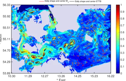
0 0.1 0.2 0.3 0.4 0.5 0.6 0.7 0.8 0.9 1 Eddy shape and center M
V Eddy shape and center ETTB
Figure 11.MVfor the western Baltic Sea for 11 May 2009 at 01:00 LT withτ=36 h normalized to the maximum value ofMV. The red lines are the eddy boundaries, and red dots the eddy cores detected with the method based onMV. The black lines are the eddy boundaries
detected with the ETTB by Nencioli et al. (2010) on 11 May 2009 at 01:00 LT. The black dots are the eddy cores detected with the ETTB by Nencioli et al. (2010) within the time interval of 11 May 2009 at 01:00 LT±36 h. The dark blue regions are areas where the trajectories have left the domain of interest; light grey regions indicate land.
surges, the North Sea–Baltic Sea model was nested into a depth-averaged storm surge model of the North Atlantic with a resolution of 5 nautical miles. The atmospheric forcing was derived from the operational model of the German Weather Service with a spatial resolution of 7 km and temporal reso-lution of 3 h. A more detailed description of the model sys-tem is given by Gräwe et al. (2015a). The flow fields for May 2009 were taken out of a running simulation covering the period 1948–2015. The velocity field was interpolated to an equidistant spacing of 1 m and finally averaged over the upper 10 m to produce a “quasi”-two-dimensional field. The temporal resolution was set to 1 h to resolve, for instance, inertial oscillations.
We have calculated MV for 11 May 2009 at 01:00 LT withτ=36 h and applied the eddy tracking based onMV. A
τ value of 36 h corresponds to 15 % of an eddy lifetime of ap-proximately 10–12 days, which was reported previously by Fennel (2001). In contrast to the test case of the vortex street, we do not expect that the eddies are perfectly circular. To ac-count for deformed and distorted eddies, we had to introduce a threshold for the convexity deficiency to eliminate contours that are only made out of filaments and are not an eddy in the sense of oceanography. We set the threshold to an 11 % dif-ference between the area of the convex hull of the points that form the boundary and the area enclosed by the boundary itself normalized to the area enclosed by the boundary. This definition of convexity deficiency is according to Haller et al. (2016). Please note that we still allow detecting contours that cover eddy merging and decay processes, which are charac-terized by filaments.
Figure 11 shows the eddy boundaries detected with the method based onMV(red) and the ETTB by Nencioli et al.
(2010) (black) on 11 May 2009 at 01:00 LT for the same search window size. There are several differences between the number and shapes of eddies which must be explained. One hundred fifty eddies can be detected with the method based onMV, whereas the ETTB detects only 24 eddies at the same instant of time. One reason for the differences is thatMV contains the information of the velocity field of a time interval, namely 11 May 2009 at 01:00 LT±36 h. Each eddy that exists, starts to arise, merges with another eddy or dies within this time interval leaves a footprint inMV like the many small eddies visible inMV. How visible this foot-print is in MV depends on the choice of τ. Therefore, the number of eddies detected with the method based onMVhas to be compared with the number of eddies detected with the ETTB by Nencioli et al. (2010) in the whole time interval that is covered byMV.
The black dots in Fig. 11 are the eddy cores detected with the ETTB by Nencioli et al. (2010) within the time interval of 11 May 2009 at 01:00 LT±36 h. In total, 339 eddies are detected which exist between<1 h and 72 h. For some eddies we will discuss exemplarily why they are detected by one of the methods and not by the other to illustrate which different problems have to be taken into account if one interprets the results of the different methods.
are detected by the ETTB by Nencioli et al. (2010) for the whole time interval; probably the eddy is too weak and lives too briefly to be seen as a structure in MV. In the case of eddy 5 the method based on MV does not detect an eddy, although the ETTB by Nencioli et al. (2010) detects several eddy cores in the region. One reason could be that the eddy arises, moves a lot and dies within the time interval such that
MV only captures a blurred structure of the eddy that does not fulfil the convexity criterion. Eddy 6 is not detected by the method based onMV, although the eddy boundary is obvious in the structure ofMV. The reason is that the choice of the search window size for the eddy core detection determines if an eddy core is detected or not. An enlarged search win-dow could solve this problem for eddy 6, but a larger search window influences the number of detected eddies. A solu-tion could be an eddy core search independent of the search window size.
A general problem which arises when using surface ve-locity fields is that this veve-locity field is not divergence-free. Although we have checked that the vertical velocity is small compared to the horizontal ones, there is still a finite resid-ual left. However, we still assume that the velocities are two-dimensional. Applying the ETTB by Nencioli et al. (2010) to these quasi-2-D fields does not cause difficulties, since the al-gorithm works on an instantaneous snapshot – a frozen veloc-ity field. Thus, the error made by the 2-D assumption is small. The situation changes when employing a Lagrangian de-scriptor. During the integration interval [t∗−τ t∗+τ],MV accumulates these residuals. Therefore,MVcan show struc-tures that seems to be eddies but are regions of a stronger ver-tical velocity or Lagrangian divergence (Jacobs et al., 2016). Therefore, the number of eddies of both methods will include false positives.
In summary, the method based on the Lagrangian descrip-torMVcan be used for the detection of eddy boundaries that act as boundaries of a trapping region. Comparing the lat-ter to boundaries detected with the ETTB by Nencioli et al. (2010) leads to large differences in the shape and in the size. Those deviations are due to the difference in the definition of the boundary. In the case of the vortex street the eddy sizes detected by the ETTB by Nencioli et al. (2010) are much smaller than the sizes detected by the method based on the Lagrangian descriptorMV. Another advantage of the method based on the Lagrangian descriptorMVis that it even shows filament structures of the eddy boundary in contrast to the ETTB by Nencioli et al. (2010) visible in the example of the western Baltic Sea. These filaments can be linked to the dy-namics of the eddy, e.g. as it starts interacting, merging or repelling with other eddies or fading out. Though these fil-ament shapes of eddies might not be eddies according to a stricter mathematical definition of an eddy boundary as in Branicki et al. (2011) and Haller et al. (2016), they are still important structures in the flow from an oceanographic point of view and should be considered in a census of eddies.
Nevertheless, one has to take into account that the detec-tion of eddy shapes by the method based on the Lagrangian descriptorMVis restricted by the choice ofτ. In highly dy-namical velocity fields like the example of the Baltic Sea not all structures can be resolved by the sameτ, which leads to a compromise forτ. This choice ofτ influences if an eddy can be detected by the method based onMV and not by the ETTB by Nencioli et al. (2010) or the other way round.
The method to detect shapes should be chosen based on which type of shapes one is interested in, and the results of the method should be handled with care.
5 Discussion and conclusion
We have shown that the Lagrangian descriptor MV based on the modulus of vorticity provides good insight into the structure of a hydrodynamic flow. It can be used to iden-tify eddy cores as well as distinguished hyperbolic trajec-tories. Eddy cores can be found as local maxima of MV, while DHTs correspond to minima ofMV. Hence, compared to the Lagrangian descriptorM based on the arc length, it does not need an additional criterion to distinguish between eddy cores and DHTs. Similar to any other Lagrangian de-scriptor, it displays singular lines that can be linked to the stable and unstable manifolds of the DHTs, which allows for a simultaneous estimate of the boundaries of the eddies to get an assessment of their size and shape. These features make the quantityMVsuitable for designing an eddy tracking tool which should be able to detect eddy cores; to track them over time; and additionally to provide information about the ed-dies’ lifetime, size and shape. Moreover, the eddy tracking should be robust with respect to velocity fields corroborated with errors when the velocity field is extracted from observa-tions.
To test all those properties in practice, we have first used some velocity fields which are constructed in such a way that the lifetimes of eddies are given analytically. It turns out that the Lagrangian descriptorMV is superior in estimating life-times compared to the other considered methods. This is due to its definition as an integral which takes the history into ac-count. Eulerian methods like Okubo–Weiss or the ETTB by Nencioli et al. (2010) detect eddies too late and underesti-mate their lifetime. The formulation ofMVas an integral is also beneficial in the case of different types of noise. How-ever, none of the tested methods can deal in a convincing way with type 3 noise which mimics errors to shifts in georefer-encing.
A general problem of any Lagrangian descriptor including
The example of the velocity field of the western Baltic Sea shows that eddy tracking based onMV is able to detect the essential eddies that are visible in the velocity field and also detected by the ETTB by Nencioli et al. (2010). Furthermore, it detects eddies that cannot be detected by the ETTB at this instant of timet∗ but was or will be detected by the ETTB at an earlier or later instant of time within the time interval [t∗−τ t∗+τ]. Nevertheless, one has to be aware that both the ETTB and the eddy tracking based onMVgive false pos-itives. The reason could be that structures of strong vertical velocity are identified as eddies. On the other hand false neg-atives can arise if (i) the eddies are too weak, (ii) the chosen
τ value is too large or too small or (iii) the search window is too large or too small.
In general, the choice of the detection method depends on the questions asked. If one is only interested in tracking eddy cores, Eulerian methods are a good choice. By contrast, La-grangian methods give a more detailed view of the dynamics and provide a more physical estimate of the eddy size. Espe-cially this feature, which describes the fluid volume trapped in an eddy, promises to be more useful for applications that consider the growth of plankton populations in oceanic flows. For the latter it has been shown that eddies can act as incuba-tors for plankton blooms due to the confinement of plankton inside the eddy (Oschlies and Garçon, 1999; Martin, 2003; Sandulescu et al., 2007).
The Supplement related to this article is available online at doi:10.5194/npg-23-159-2016-supplement.
Author contributions. Rahel Vortmeyer-Kley developed the idea of the eddy tracking tool based on the Lagrangian descriptorMVand implemented it. Ulf Gräwe supervised the oceanic questions of this work and provided the velocity field for the western Baltic Sea. The overall supervision was done by Ulrike Feudel. All authors con-tributed in preparing this manuscript.
Acknowledgements. Rahel Vortmeyer-Kley would like to thank the Studienstiftung des Deutschen Volkes for a doctoral fellowship. The financing of further developments of the Leibniz Institute of Baltic Sea Research monitoring programme and adaptations of nu-merical models (STB-MODAT) by the federal state government of Mecklenburg-Vorpommern is greatly acknowledged by Ulf Gräwe. The authors would like to thank Jan Freund, Ana Mancho, Matthias Schröder, Wenbo Tang, Tamás Tél and Alfred Ziegler for stimulating discussions.
Edited by: A. M. Mancho
Reviewed by: K. McIlhany and two anonymous referees
References
Abraham, E. R.: The generation of plankton patchiness by turbulent stirring, Nature, 391, 577–580, 1998.
Artale, V., Boffetta, G., Celani, M., Cencini, M., and Vulpiani, A.: Dispersion of passive tracers in closed basins: Beyond the diffu-sion coeffcient, Phys. Fluids, 9, 3162–3171, 1997.
Bastine, D. and Feudel, U.: Inhomogeneous dominance patterns of competing phytoplankton groups in the wake of an island, Non-lin. Processes Geophys., 17, 715–731, doi:10.5194/npg-17-715-2010, 2010.
Bettencourt, J. H., López, C., and Hernández-García, E.: Oceanic three-dimensional Lagrangian coherent structures: A study of a mesoscale eddy in the Benguela upwelling region, Ocean Model., 51, 73–83, 2012.
Boffetta, G., Lacorata, G., Redaelli, G., and Vulpiani, A.: Detecting barriers to transport: a review of different techniques, Physica D, 159, 58–70, 2001.
Bracco, A., Provenzale, A., and Scheuring, I.: Mesoscale vortices and the paradox of the plankton, P. Roy. Soc. Lond. B, 267, 1795–1800, 2000.
Branicki, M. and Wiggins, S.: Finite-time Lagrangian transport analysis: stable and unstable manifolds of hyperbolic trajecto-ries and finite-time Lyapunov exponents, Nonlin. Processes Geo-phys., 17, 1–36, doi:10.5194/npg-17-1-2010, 2010.
Branicki, M., Mancho, A., and Wiggins, S.: A Lagrangian descrip-tion of transport associated with a front-eddy interacdescrip-tion: Appli-cation to data from the North-Western Mediterranean Sea, Phys-ica D, 240, 282–304, 2011.
Chaigneau, A., Gizolme, A., and Grados, C.: Mesoscale eddies off Peru in altimeter records: Identification algorithms and eddy spatio-temporal patterns, Prog. Oceanogr., 79, 106–119, 2008. Chelton, D. B., Schlax, M. G., and Samelson, R. M.: Global
ob-servations of nonlinear mesoscale eddies, Prog. Oceanogr., 91, 167–216, 2011.
de la Cámara, A., Mancho, A. M., Ide, K., Serrano, E., and Me-choso, C. R.: Routes of Transport across the Antarctic Polar Vor-tex in the Southern Spring, J. Atmos. Sci., 69, 741–752, 2012. Dong, C., Idica, E. Y., and McWilliams, J. C.: Circulation and
multiple-scale variability in the Southern California Bight, Prog. Oceanogr., 82, 168–190, 2009.
Dong, C., Lin, X., Liu, Y., Nencioli, F., Chao, Y., Guan, Y., Chen, D., Dickey, T., and McWilliams, J. C.: Three-dimensional oceanic eddy analysis in the Southern California Bight from a numerical product, J. Geophys. Res., 117, C00H14, doi:10.1029/2011JC007354, 2012.
Dong, C., McWilliams, J. C., Liu, Y., and Chen, D.: Global heat and salt transports by eddy movement, Nat. Commun., 5, 1–6, 2014. Donlon, C. J., Martin, M., Stark, J., Roberts-Jones, J., Fiedler, E., and Wimmer, W.: The Operational Sea Surface Temperature and Sea Ice Analysis (OSTIA) system, Remote Sens. Environ., 116, 140–158, 2012.
Douglass, E. M. and Richman, J. G.: Analysis of ageostrophy in strong surface eddies in the Atlantic Ocean, J. Geophys. Res.-Oceans, 120, 1490–1507, 2015.
Eugenio, F. and Marqués, F.: Automatic Satellite Image Georefer-encing Using a Contour-Matching Approach, IEEE T. Geosci. Remote, 41, 2869–2880, 2003.
Fennel, K.: The generation of phytoplankton patchiness by mesoscale current patterns, Ocean Dynam., 52, 58–70, 2001. Fernandes, M. A., Nascimento, S., and Boutov, D.: Automatic
iden-tification of oceanic eddies in infrared satellite images, Comput. Geosci., 37, 1783–1792, 2011.
Froyland, G. and Padberg, K.: Almost-invariant sets and invari-ant manifolds – Connecting probabilistic and geometric descrip-tions of coherent structures in flows, Physica D, 238, 1507–1523, 2009.
García-Garrido, V. J., Mancho, A. M., Wiggins, S., and Mendoza, C.: A dynamical systems approach to the surface search for de-bris associated with the disappearance of flight MH370, Non-lin. Processes Geophys., 22, 701–712, doi:10.5194/npg-22-701-2015, 2015.
Gawlik, E. S., Marsden, J. E., Du Toit, P. C., and Campagnola, S.: Lagrangian coherent structures in the planar elliptic restricted three-body problem, Celest. Mech. Dyn. Astr., 103, 227–249, 2009.
Gräwe, U., Holtermann, P., Klingbeil, K., and Burchard, H.: Ad-vantages of vertically adaptive coordinates in numerical models of stratified shelf seas, Ocean Model., 92, 56–68, 2015a. Gräwe, U., Naumann, M., Mohrholz, V., and Burchard, H.:
Anat-omizing one of the largest saltwater inflows into the Baltic Sea in December 2014, J. Geophys. Res.-Oceans., 120, 7676–7697, 2015b.
Haller, G.: Lagrangian Coherent Structures, Annu. Rev. Fluid Mech., 47, 137–162, 2015.
Haller, G. and Beron-Vera, F.: Coherent Lagrangian vortices: the black holes of turbulence, J. Fluid Mech., 731, R4, doi:10.1017/jfm.2013.391, 2013.
Haller, G. and Yuan, G.: Lagrangian coherent structures and mixing in two-dimensional turbulence, Physica D, 147, 352–370, 2000. Haller, G., Hadjighasem, A., Farazmand, M., and Huhn, F.:
Defin-ing coherent vortices objectively from the vorticity, J. Fluid Mech., 795, 136–173, 2016.
Hernández-Carrasco, I., Rossi, V., Hernández-García, E., Garçon, V., and López, C.: The reduction of plankton biomass induced by mesoscale stirring: A modeling study in the Benguela upwelling, Deep-Sea Res. Pt. I, 83, 65–80, 2014.
Huhn, F., Kameke, A., Pérez-Muñuzuri, V., Olascoaga, M., and Beron-Vera, F.: The impact of advective transport by the South Indian Ocean Countercurrent on the Mada-gaskar plankton bloom, Geophys. Res. Lett., 39, L06602, doi:10.1029/2012GL051246, 2012.
Ide, K., Small, D., and Wiggins, S.: Distinguished hyperbolic tra-jectories in time-dependent fluid flows: analytical and computa-tional approach for velocity fields defined as data sets, Nonlin. Processes Geophys., 9, 237–263, doi:10.5194/npg-9-237-2002, 2002.
Isern-Fontanet, J., García-Ladona, E., and Font, J.: Vortices of the Mediterranean Sea: An Altimetric Perspective, J. Phys. Oceanogr., 36, 87–103, 2006.
Jacobs, G. A., Huntley, H. S., Kirwan, A., Lipphardt, B. L., Camp-bell, T., Smith, T., Edwards, K., and Bartels, B.: Ocean pro-cesses underlying surface clustering, J. Geophys. Res.-Oceans, 121, 180–197, 2016.
Jung, C., Tél, T., and Ziemniak, E.: Application of scattering chaos to particle transport in a hydrodynamical flow, Chaos, 3, 555– 568, 1993.
Karrasch, D., Huhn, F., and Haller, G.: Automated detection of co-herent Lagrangian vortices in two-dimensional unsteady flows, P. Roy. Soc. A, 471, 20140639, doi:10.1098/rspa.2014.0639, 2015. Klingbeil, K., Mohammadi-Aragh, M., Gräwe, U., and Burchard, H.: Quantification of spurious dissipation and mixing – Discrete variance decay in a Finite-Volume framework, Ocean Model., 81, 49–64, 2014.
Koh, T. Y. and Legras, B.: Hyperbolic lines and the stratospheric polar vortex, Chaos, 12, 382–394, 2002.
Leprince, S., Barbot, S., Ayoub, F., and Avouac, J. P.: Automatic and precise orthorectification, coregistration, and subpixel cor-relation of satellite images, application to ground deformation measurements, IEEE T. Geosci. Remote, 45, 1529–1558, 2007. Madrid, J. A. J. and Mancho, A. M.: Distinguished
trajec-tories in time dependent vector fields, Chaos, 19, 013111, doi:10.1063/1.3056050, 2009.
Mahoney, J., Bargteil, D., Kingsbury, M., Mitchell, K., and Solomon, T.: Invariant barriers to reactive front propagation in fluid flows, Europhys. Lett., 98, 44005, doi:10.1209/0295-5075/98/44005, 2012.
Mahoney, J. R. and Mitchell, K. A.: Finite-time barriers to front propagation in two-dimensional fluid flows, Chaos, 25, 087404, doi:10.1063/1.4922026, 2015.
Mancho, A., Small, D., and Wiggins, S.: A tutorial on dynami-cal systems concepts applied to Lagrangian transport in oceanic flows defined as finite time data sets: Theoretical and computa-tional issues, Phys. Rep., 437, 55–124, 2006.
Mancho, A., Wiggins, S., Curbelo, J., and Mendoza, C.: Lagrangian Descriptors: A method of revealing phase space structures of general time dependent dynamical systems, Commun. Nonlin. Sci., 18, 3530–3557, 2013.
Martin, A.: Phytoplakton patchiness: the role of lateral stirring and mixing, Prog. Oceanogr., 57, 125–174, 2003.
Martin, A., Richards, K., Bracco, A., and Provenzale, A.: Patchy productivity in the open ocean, Global Biogeochem. Cy., 16, 9-1–9-9, doi:10.1029/2001GB001449, 2002.
McIlhany, K. and Wiggins, S.: Eulerian indicators under con-tinuously varying conditions, Phys. Fluids, 24, 073601, doi:10.1063/1.4732152, 2012.
McIlhany, K., Mott, D., Oran, E., and Wiggins, S.: Optimizing mix-ing in lid-driven flow designs through predictions from Eulerian indicators, Phys. Fluids, 23, 082005, doi:10.1063/1.3626022, 2011.
McIlhany, K., Guth, S., and Wiggins, S.: Lagrangian and Eule-rian analysis of transport and mixing in the three dimensional, time dependent Hill’s spherical vortex, Phys. Fluids, 27, 063603, doi:10.1063/1.4922539, 2015.
Mendoza, C. and Mancho, A.: Hidden geometry
of ocean flows, Phys. Rev. Lett., 105, 038501, doi:10.1103/PhysRevLett.105.038501, 2010.
Mendoza, C. and Mancho, A. M.: Review Article: “The La-grangian description of aperiodic flows: a case study of the Kuroshio Current”, Nonlin. Processes Geophys., 19, 449–472, doi:10.5194/npg-19-449-2012, 2012.
al-timeter velocity fields, Nonlin. Processes Geophys., 17, 103–111, doi:10.5194/npg-17-103-2010, 2010.
Mezi´c, I., Loire, S., Fonoberov, V. A., and Hogan, P.: A New Mixing Diagnostic and Gulf Oil Spill Movement, Science, 330, 486–489, 2010.
Mitchell, K. A. and Mahoney, J. R.: Invariant manifolds and the geometry of front propagation in fluid flows, Chaos, 22, 037104, doi:10.1063/1.4746039, 2012.
Morrow, R. and Le Traon, P.-Y.: Recent advances in observing mesoscale ocean dynamics with satellite altimetry, Adv. Space Res., 50, 1062–1076, 2012.
Nencioli, F., Dong, C., Dickey, T., Washburn, L., and McWilliams, J. C.: A Vector Geometry-Based Eddy Detection Algorithm and Its Application to a High-Resolution Numerical Model Product and High-Frequency Radar Surface Velocities in the Southern California Bight, J. Atmos. Ocean. Tech., 27, 564–579, 2010. Okubo, A.: Horizontal dispersion of floatable particles in the
vicin-ity of velocvicin-ity singularities such as convergences, Deep-Sea Res. Oceanogr. Abstr., 17, 445–454, 1970.
Olascoaga, M. J. and Haller, G.: Forecasting sudden changes in en-vironmental pollution patterns, P. Natl. Acad. Sci. USA, 109, 4738–4743, 2012.
Onu, K., Huhn, F., and Haller, G.: LCS Tool: A Computational Plat-form for Lagrangian Coherent Structures, J. Comput. Sci., 7, 26– 36, 2015.
Oschlies, A. and Garçon, V.: An eddy-permitting coupled physical-biological model of the North-Atlantic, sensitivity to advection numerics and mixed layer physics, Global Biogeochem. Cy., 13, 135–160, 1999.
Petersen, M. R., Williams, S. J., Maltrud, M. E., Hecht, M. W., and Hamann, B.: A three-dimensional eddy census of a high-resolution global ocean simulation, J. Geophys. Res.-Oceans, 118, 1759–1774, 2013.
Rossi, V., López, C., Sudre, J., Hernández-García, E., and Garçon, V.: Comparative study of mixing and biological activity of the Benguela and Canary upwelling systems, Geophys. Res. Lett., 35, L11602, doi:10.1029/2008GL033610, 2008.
Sadarjoen, I. A. and Post, F. H.: Detection, quantification, and track-ing of vortices ustrack-ing streamline geometry, Comput. Graph., 24, 333–341, 2000.
Sandulescu, M., Hernández-García, E., López, C., and Feudel, U.: Kinematic studies of transport across an island wake, with appli-cation to Canary islands, Tellus A, 58, 605–615, 2006.
Sandulescu, M., López, C., Hernández-García, E., and Feudel, U.: Plankton blooms in vortices: the role of biological and hydro-dynamic timescales, Nonlin. Processes Geophys., 14, 443–454, doi:10.5194/npg-14-443-2007, 2007.
Sturman, R. and Wiggins, S.: Eulerian indiators for predicting and optimazing mmixing quality, New J. Phys., 11, 075031, doi:10.1088/1367-2630/11/7/075031, 2009.
Tang, W. and Luna, C.: Dependence of advection-diffusion-reaction on flow coherent structures, Phys. Fluids, 25, 106602, doi:10.1063/1.4823991, 2013.
Thacker, W. C., Lee, S.-K., and Halliwell, G. R.: Assimilating 20 years of Atlantic XBT data into HYCOM: a first look, Ocean Model., 7, 183–210, 2004.
Weiss, J.: The dynamics of enstrophy transfer in two-dimensional hydrodynamics, Physica D, 48, 273–294, 1991.
Wiggins, S.: The dynamical systems approach to Lagrangian transprt in oceanic flows, Annu. Rev. Fluid Mech., 37, 295–328, 2005.
Wiggins, S. and Mancho, A. M.: Barriers to transport in aperiodi-cally time-dependent two-dimensional velocity fields: Nekhoro-shev’s theorem and “Nearly Invariant” tori, Nonlin. Processes Geophys., 21, 165–185, doi:10.5194/npg-21-165-2014, 2014. Wilson, M. M., Peng, J., Dabiri, J. O., and Eldredge, J. D.:
La-grangian coherent structures in low Reynolds number swim-ming, J. Phys.-Condens Mat., 21, 204105, doi:10.1088/0953-8984/21/20/204105, 2009.
Wischgoll, T. and Scheuermann, G.: Detection and visualization of closed streamlines in planar flows, IEEE T Vis Compu Gr, 7, 165–172, 2001.