RESEARCH ARTICLE
Population Size Predicts Lexical Diversity, but
so Does the Mean Sea Level
–
Why It Is
Important to Correctly Account for the
Structure of Temporal Data
Alexander Koplenig*, Carolin Müller-Spitzer
Department of Lexical Studies, Institute for the German language (IDS), Mannheim, Germany
*Koplenig@ids-mannheim.de
Abstract
In order to demonstrate why it is important to correctly account for the (serial dependent) structure of temporal data, we document an apparently spectacular relationship between population size and lexical diversity: for five out of seven investigated languages, there is a strong relationship between population size and lexical diversity of the primary language in this country. We show that this relationship is the result of a misspecified model that does not consider the temporal aspect of the data by presenting a similar but nonsensical rela-tionship between the global annual mean sea level and lexical diversity. Given the fact that in the recent past, several studies were published that present surprising links between dif-ferent economic, cultural, political and (socio-)demographical variables on the one hand and cultural or linguistic characteristics on the other hand, but seem to suffer from exactly this problem, we explain the cause of the misspecification and show that it has profound consequences. We demonstrate how simple transformation of the time series can often solve problems of this type and argue that the evaluation of the plausibility of a relationship is important in this context. We hope that our paper will help both researchers and reviewers to understand why it is important to use special models for the analysis of data with a natural temporal ordering.
Introduction
In principle, we could start our paper like this: As complex adaptive systems [1], languages are constantly changing on all fundamental levels [2]. In this context, several studies have indicated that population size is an important factor that influences the (rate of) language change [3–5]. Based on a very large sample of the written language record [6], we present quantitative evi-dence that clearly supports the claim that population size strongly influences the lexical diver-sity of eight languages. The problem is: an almost identical pattern emerges if we correlate the lexical diversity in a given year with the global mean sea level [7] instead of population size. This strongly raises the suspicion that there might be something wrong with our analysis. The OPEN ACCESS
Citation:Koplenig A, Müller-Spitzer C (2016) Population Size Predicts Lexical Diversity, but so Does the Mean Sea Level–Why It Is Important to Correctly Account for the Structure of Temporal Data. PLoS ONE 11(3): e0150771. doi:10.1371/journal. pone.0150771
Editor:Karen Lidzba, University Children's Hospital Tuebingen, GERMANY
Received:October 26, 2015
Accepted:February 17, 2016
Published:March 3, 2016
Copyright:© 2016 Koplenig, Müller-Spitzer. This is an open access article distributed under the terms of theCreative Commons Attribution License, which permits unrestricted use, distribution, and reproduction in any medium, provided the original author and source are credited.
Data Availability Statement:All relevant data are within the paper and its Supporting Information files.
Funding:The publication of this article was funded by the Open Access fund of the Leibniz Association.
description of this problem and its consequences are at the very heart of our study: we show that whenever two variables evolve through time, those variables will almost always look highly correlated even if they are not related in any substantial sense. While we want to point out upfront that the problem is fairly common knowledge in econometric time-series analysis [8–
11], we nevertheless felt the need to outline it once again, in an instructive and non-technical manner, in this paper, given the fact that in the recent past, several studies were published–
some in journals with a good reputation–that seem to suffer from exactly this problem [12–
18]. Following [19], we consider the fact that those studies do not correctly account for the temporal structure of the data problematic, because the studies sometimes present surprising or even spectacular relationships, especially between different economic, cultural, political and (socio-)demographical variables on the one hand and cultural or linguistic characteristics (like the one described above) on the other hand. As a result, the studies also receive widespread media attention and can, in turn, affect public opinion and decision making. We therefore hope that our paper can help both researchers and reviewers detect the problem and ultimately avoid it.
The remainder of this paper is organized in the following way: First, we document an appar-ently spectacular relationship between population size and lexical diversity. We then try to show that this relationship is the result of a misspecified model that does not correctly account for the (serial dependent) structure of temporal data of the data by presenting a similar but nonsensical relationship between the global annual mean sea level and lexical diversity. On this basis, we explain the cause of the misspecification, show that it has profound consequences and demonstrate how simple data transformation can often solve the problem, before arguing that checking for plausibility is important in this context. This paper ends with some concluding remarks.
Results and Discussion
The problem of spurious correlations
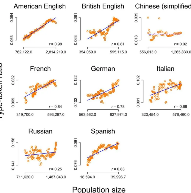
We‘investigated’the correlation between population size and lexical diversity for American English, British English, Chinese (simplified), French, German, Italian, Russian and Spanish on the basis of data on population size and the type-token ratio based on the Google Books dataset (seeMaterials and Methodsfor more details). At first glance,Fig 1seems to document a spectacular and fascinating relationship: There is a strong and statistically significant correla-tion (atp<.05 or better) between the level of the population size and the level of the
type-token ratio as a measure of lexical diversity for all investigated languages, except Chinese. On this basis, we could argue for a general relationship. For example, we assume that with increas-ing populations, the number of language speakers naturally also increases. We could then con-tinue and elaborate our argument by assuming that a larger number of speakers is most likely associated with a greater degree of variance in demographic background and sociocultural environments [20], and that this greater diversity leads to an increase of the type-token ratio as a measure of lexical diversity. The fact that there is virtually no correlation for Chinese and–
compared to the other languages–only a small correlation for the Russian data could then be incorporated in our "theory" by referring to the political background in those two countries, e.g. that in socialist countries, increasing population sizes do not affect the lexical diversity, because socialist coercion policies suppresses linguistic development by defining one common "linguistic" or "cultural" standard or something like that. This is exactly what [19] alerted to, since this result could be used in the media or even by politicians to criticize socialism.
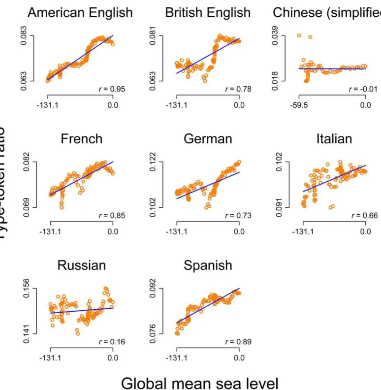
possible to argue for, the relationship between the global mean sea level and the lexical diversity is highly similar. In this context, all correlations except for Chinese and Russian are strong and highly significant (atp<.001 or better). However, arguing for any potential relationship seems to be out of the question in this context.
Fig 1. Correlation between the level of the population size and the level of the type-token ratio for eight languages (including two varieties of English).Orange circles: raw data. Blue line: linear prediction of the type-token ratio on the population size. Notes on the bottom right: Pearson correlation (allps<.05 or better, except for Chinese wherep= .89).
doi:10.1371/journal.pone.0150771.g001
Fig 3"explains" these apparent relationships: all type-token ratio time-series, again except for Chinese and Russian, clearly exhibit an upward trend. The series are said to have a unit root or to be non-stationary [11]. The same is true for both the population sizes and the global mean sea level, which also increased throughout the 20thcentury. For the analysis of temporal Fig 2. Correlation between the level of the annual global mean seal level and the level of the type-token ratio for eight languages (including two varieties of English).Orange circles: raw data. Blue line: linear prediction of the type-token ratio on the population size. Notes on the bottom right: Pearson correlation (allps<.001 except for Chinese werep= 0.95 and Russian wherep= .10)
data, this has important ramifications because the following statement is trueper definition: values that are later in time will be above the average of the mean value of the series, while val-ues that are earlier in time will be below average. Since the Pearson product-moment correla-tion measures whether values of one series that are above/below average tend to co-occur with values of another series that are above/below average, by mathematical necessity, the
Fig 3. Type-token ratio as a function of time for eight languages (including two varieties of English).Orange lines: raw data. Blue lines: simple weighted moving average with an 11-year window centered on the current value.
doi:10.1371/journal.pone.0150771.g003
correlation coefficient for two trending time-series will then be high when in fact they are not related in any substantial sense [8]. An augmented Dickey-Fuller test (a formal test for a unit root) with a lag length of 1 reveals that all time series that include the population sizes and the global mean sea level are non-stationary (allps>.05), except for the Chinese and the Russian type-token ration series wherep<.05.
Changes instead of levels
One common approach to avoid spurious correlations is to transform the series prior to the analysis, for example by detrending the series (estimating the trend and subtracting it from the actual series). Another more general solution that often results in stationary series, that is a series in which the mean and the variance of the investigated series do not change as a function of time, is to correlate period-to-period changes instead of the actual levels of the two series [11]. It is worth emphasizing that this also re-formulates the research question as it excludes the upward trends of the correlated series [21]. It determines if period-to-period changes that are above or below the average of the first series correspond mainly to changes that are above or below the average of the second series. Therefore, [8] suggest as a rule of thumb to generally model data on a combination of both levels and changes. In our case, correlating year-to-year changes (or decade-to-decade changes) seems to be even better suited to answer our "research question": if the population increases from last year to this year, then–on average–lexical diver-sity should also increase from last year to this year, if both series are related. If we correlate year-to-year changes all correlations between population size / global mean sea level and lexical diversity become virtually nonexistent (rmax= .10) and insignificant at all common levels of
sig-nificance (pmin= .31).
The problem of temporal autocorrelation
To demonstrate why it is problematic to correlate two trending time-series, we have simulated 10,000 random walks with drift (cf. Materials and Methods). Each resulting time-series has an average upward trend, but otherwise behaves in a completely random manner. This means that the random walks serve as a proxy for time series with a general upward trend. All series are then correlated with the annual global mean sea level.Fig 4shows that 7,519 of the 10,000 ran-dom walks correlate moderately (r>.30) and more than 50% (5,432) even correlate strongly
(r>.75) with the global mean sea level, if we calculate the correlation based on the level of the series (rmean= .52). This result is, of course, far from what we should actually expect for the
dis-tribution of correlation coefficients where one variable is a random quantityper definition: only a few series should–by chance–substantially correlate with the global mean sea level, while most correlation coefficients should be close to zero. If we instead correlate year-to-year changes of the two series, the maximum correlation coefficients amounts tor= .37 and–as expected–a distribution that closely resembles a normal distribution (blue line inFig 4) with a mean close to zero (rmean= .00).
Fig 4. Correlations between the annual global mean seal level and 10,000 simulated random walks with drift.Top: Histogram of the correlations between levels. Bottom: Histogram of the correlation between year-to-year changes. The height of the bars in both histograms represents the number of cases in the category. Blue lines: scaled normal density.
doi:10.1371/journal.pone.0150771.g004
Plausibility
To demonstrate why it is also important–especially for a spectacular and unexpected result–to remain skeptical and to carefully check plausibility, let us briefly give an example what our ini-tial“analysis”of the relationship between lexical diversity and population size would actually imply: if we regress the level of the lexical diversity in the Spanish Google Books data on the population size of Spain, we obtain a coefficient of determination ofr2= .69. This means that almost 70% of the variance of the lexical diversity variable is“explained”by the population size (for the American English data it would be even more than 95% of the variance). This model would also imply that every 10 new inhabitants of Spain are equal to 4.56 additional word types (per 1 million word tokens) in the Spanish Google Books data (that also includes books written and published in Latin America). We believe that this would be an extraordinary result. In fact, this result would be so extraordinary that it seems wise to first ask: is this result plausi-ble? Can we come up with any good theory regarding this relationship?
A few words on the Google Books data are in order here, as they are the basis of all but one [16] study quoted above. Here, we want to echo ([22], p. 1203): just because a dataset is big, does not mean that“one can ignore foundational issues of measurement and construct validity and reliability and dependencies among data.”However, this seems to be precisely the case regarding the Google Books Ngram data. After all, forn-grams wherenis ranges from one (single words) to five (five word units), the data consist of only year-wise aggregated overall fre-quencies of occurrence and the number of books each n-gram appears in. Since n-grams do not occur independently across distinct books, this aggregation of individual book frequencies means that we cannot account for the distributions of n-grams which can have profound con-sequences for the analysis of textual data [23,24]. In addition, it is a largely overlooked fact that the Google Books Ngram data only includes the counts for n-grams that occur at least 40 times across the entire corpus. At least from a (corpus) linguistic point of view, this certainly matters since most n-grams are very infrequent. So in terms of what we know about word frequency dis-tributions [25], this procedure eliminates approximately 95% of all different 1-gram types; for n-grams where n>1 this figure is even higher [26]. To the best of our knowledge, the question of whether this arbitrary data truncation does not impose a systematic bias on the data is something that remains to be demonstrated empirically, given the fact that corpus size for each year strongly increases as a function of time. At the same time, this means that we would have to further extend our analysis illustrated above: nearly every second new inhabitant of Spain is "responsible" for one new word typethat occurs more than 40 timesin the Spanish Google Books data.
To check the plausibility of this result, we would have to face the fact that we still do not have any reliable information about the books included in the corpora. According to the FAQs of the Culturomics project behind the GB data [27] the team has“not received permission [. . .]
Returning to our research question–the correlation between population size and lexical diversity–population growth is affected by the birth of children and the influx of immigrants. Babies do not write books, and only a few immigrants publish books which are acquired by libraries shortly after immigration. So, the strong relationship between lexical diversity and population size would indicate that nearly every second new inhabitant (babies and immigrants alike) is "responsible" for one new word typethat occurs more than 40 timesin the Spanish Google Books data. This would really be an extraordinary relationship.
To drive home this point, if we regress the level of lexical diversity in the German Google Books data to the population size of China, we obtain a very strong correlation ofr= .89 that is significant at all standard levels. Our model predicts that with every 1,000 new inhabitants of China, we will find roughly 15 additional word types in the German Google Books data. While it is certainly possible to“rationalize nearly everything”([9], p. 2), we just do not think that this result makes any sense–which mechanism could generate a relationship like this? If we use year-to-year changes instead of the actual levels, we obtain an insignificant correlation of 0.10 (p= 0.34). This implies that knowing the Chinese population size does not help in predicting the lexical diversity in the Google Books data, a result which we believe fits reality more closely.
From a statistical point of view, this demonstrates why it can be a good idea to model a potential relationship between two trending time series with changes instead of levels. This is also important from a methodological point of view: just because two series are trending, does not necessarily imply any substantial relationship [31]. Therefore we strongly advise against using the fact that two series are evolving in a predicted way as evidence in order to substantiate a specific theoretical claim.
The general question concerning the Google Books data itself, whether the acquisition strat-egy of major libraries really can serve as an (temporarily) unbiased proxy for the evolution of subjective or even latent cognitive traits, is an open research question. Again, we are rather skeptical. For example, a change in the acquisition strategy of one major library is not necessar-ily motivated by one of the factors we might be interested in; nevertheless in aggregation of the frequency counts of different n-grams, it might look like one. Once again, we want to refer to ([22], p. 1203) regarding such naïve mapping:
“All empirical research stands on a foundation of measurement. Is the instrumentation actually capturing the theoretical construct of interest? Is measurement stable and comparable across cases and over time? Are measurement errors systematic?”
The outlined problems all have to do with the fact that–in making the data freely available (which is a fantastic thing)–Google wanted to avoid breaking any copyright laws, and it goes with-out saying that legal restrictions also have to be taken seriously in this case. However, while we are–
as many other empirically-minded researchers–fascinated by the possibilities that the analysis of
“big data”offers, we believe that the seemingly prevailing view that the size of the (Google Books Ngram) data will stand in for fundamental methodological problems, is not justified.
Concluding Remarks
All recently published studies that we mentioned in the introduction do not explicitly model the underlying temporal structure of the data [12–18]. This certainly has to do with the fact that time series analysis is a relatively young statistical discipline ([11], p. xxi-xxii). To improve the reliability of research [32], we hope that this paper will help both researchers and reviewers to understand why it is important to use special models for the analysis of such data. Standard statistical models that work for cross-sectional data run the risk of incorrect statistical inference in time-series analysis, where (potentially strong) effects are meaningless and therefore can potentially lead to wrong conclusions.
While our analysis indicates that type-token ratios do not dependent on population sizes, this does not imply, of course, that the increase of the type-token ratios over time is not inter-esting in itself as Harald Baayen (personal communication) points out, because this increase could reflect the fact that onomasiological needs increase with the complexity of modern socie-ties [33]. Or put differently, new ideas and new technologies need new designations in order to efficiently communicate about related concepts. Thus, under the assumption that cultural adaption is cumulative [34,35], a rapid increase of technological innovations could result in an increase of the type-token ratio, independently of the population size. This is certainly an inter-esting avenue for future research.
Materials and Methods
S1 Filecontains the population data, compiled from [36]. The time-series of the global mean sea level was presented in [7] and is available at [37]. The type-token ratio, a common way to measure lexical diversity, is based on the Google Books datasets that were made available by [6] at [27]. For the present study, the 1-gram datasets of Version 2 (July 2012) of the following lan-guages were used: American English, British English, Chinese (simplified), French, German, Italian, Russian and Spanish. The type-token ratio for each year and each language is calculated by dividing the number of unique strings by the total number of strings. Higher type-token ratios are indicative of higher lexical diversity. Since this measure is known to be heavily text-length dependent [38] and given the fact that the corpus size based on the Google Books data strongly increases as a function of time, calculating the type-token ratio based on the actual corpus sizes would systematically bias the results. To solve this problem, random samples of 1,000,000 tokens were drawn from the data as described in [39]. The analysis is restricted to the 20thcentury, except for Chinese, which is restricted to the time span 1950–2000 since the size of the Google Books base corpora is not sufficient (<1,000,000 tokens) for earlier periods.
Additionally, we simulatedi= 10,000 random walks with drift [40,11] that are defined as:
xt;i ¼di xt 1;iþet;i
wherext,iis the value of theith random walk at time pointt; the constant drift termdiis
ran-domly drawn from a uniformly distributed interval [0.02,0.2) andet,iis white noise, normally
distributed over the interval [0,1).
For each resulting series this means that the current value of the series depends on its previ-ous value plus a positive drift term and a white noise error term. At each point in time, the series takes one random step away from the last position, but as result of the drift term, the series will have an upward trend in the long-run.
All analyses were carried out using Stata/MP2 14.0 for Windows (64-bit version). To ensure maximal replicability,S2 Filecontains a Stata script (‘do-file’) that automatically downloads the data and reproduces all results presented in this article, whileS3 Fileis a delimited text file (comma-separated) of the final dataset that can be used to replicate our findings with another software package.
Temporal autocorrelation
From a statistical point of view, temporal autocorrelation is problematic because it biases our estimators. If, for example, we fit a simple time-series regression that can be written as:
yt¼b0þb1x1tþεt
whereytrepresents the level of our outcome variable intandx1tis the level of predictor
Fig 5. Correlations of current and lagged residuals of a regression of the 10,000 simulated random walks with drift on the annual global mean seal level.Top: Histogram for levels. Bottom: Histogram for year-to-year changes. The height of the bars in both histograms represents the number of cases in the category. Blue lines: scaled normal density.
doi:10.1371/journal.pone.0150771.g005
analysis assumes that there is no autocorrelation between the residuals (Cov(εs,εt) = 0 for all s6¼t). In this context,first-order autocorrelationεtcan be written as:
εt¼rεt 1þZt
whereρis the autoregressive parameter andηtis a white-noise process. In the presence offi
rst-order autocorrelation, the OLS estimators are biased and lead to incorrect statistical inferences [41]. To see, why this is also the problem of our simulation,Fig 5shows the correlation between current and lagged residuals of an OLS regression for each of the simulated random walks with drift on the annual global mean seal level. While the regression residuals of levels are strongly autocorrelated (rmean= .91), we obtain a normal distribution with a mean close to zero (rmean=
-.02) for the regression residuals of year-to-year changes.
Supporting Information
S1 File. Population size data, compiled from [36].
(XLSX)
S2 File. Stata do-file that automatically downloads the data and reproduces all results pre-sented in the article.
(TXT)
S3 File. Delimited text file (comma-separated) of the final dataset that can be used to repli-cate our findings.
(TXT)
Acknowledgments
We would like to thank Sascha Wolfer for valuable comments on earlier drafts of this article and Sarah Signer for proofreading. Also, we are grateful to an anonymous reviewer for helpful suggestions and to Harald Baayen for insightful comments and additional inputs on the inter-pretation of our analyses as mentioned in the text. The publication of this article was funded by the Open Access fund of the Leibniz Association.
Author Contributions
Conceived and designed the experiments: AK CMS. Performed the experiments: AK. Analyzed the data: AK. Wrote the paper: AK CMS.
References
1. Beckner C, Blythe R, Bybee J, Christiansen MH, Croft W, Ellis NC, et al. Language Is a Complex Adap-tive System: Position Paper. Lang Learn. 2009; 59: 1–26. doi:10.1111/j.1467-9922.2009.00533.x 2. Labov W. Principles of linguistic change. Oxford, UK; Cambridge [Mass.]: Blackwell; 1994. 3. Bromham L, Hua X, Fitzpatrick TG, Greenhill SJ. Rate of language evolution is affected by population
size. Proc Natl Acad Sci. 2015; 112: 2097–2102. doi:10.1073/pnas.1419704112PMID:25646448 4. Nettle D. Is the rate of linguistic change constant? Lingua. 1999; 108: 119–136. doi:
10.1016/S0024-3841(98)00047-3
5. Wichmann S, Holman EW. Population Size and Rates of Language Change. Hum Biol. 2009; 81. Avail-able:http://digitalcommons.wayne.edu/humbiol/vol81/iss2/8.
6. Michel J-B, Shen YK, Aiden AP, Verses A, Gray MK, The Google Books Team, et al. Quantitative Anal-ysis of Culture Using Millions of Digitized Books. Science. 2010; 331: 176–182 [online pre–print: 1–12]. doi:10.1126/science.1199644PMID:21163965
8. Granger CWJ, Newbold P. Spurious regressions in econometrics. J Econom. 1974; 2: 111–120. doi: 10.1016/0304-4076(74)90034-7
9. Yule GU. Why do we sometimes get nonsense correlations between time series? A study in sampling and the nature of time series. J R Stat Soc. 1926; 89: 1–64.
10. Chatfield C. The analysis of time series: an introduction. 6th ed. Boca Raton, FL: Chapman & Hall/ CRC; 2004.
11. Becketti S. Introduction to time series using Stata. 1st ed. College Station, Tex: Stata Press; 2013. 12. Bentley RA, Acerbi A, Ormerod P, Lampos V. Books Average Previous Decade of Economic Misery.
Perc M, editor. PLoS ONE. 2014; 9: e83147. doi:10.1371/journal.pone.0083147PMID:24416159 13. Caruana-Galizia P. Politics and the German language: Testing Orwell’s hypothesis using the Google
N-Gram corpus. Digit Scholarsh Humanit. 2015; doi:10.1093/llc/fqv011
14. Hills TT, Adelman JS. Recent evolution of learnability in American English from 1800 to 2000. Cogni-tion. 2015; 143: 87–92. doi:10.1016/j.cognition.2015.06.009PMID:26117487
15. Hills T, Protio E, Sgroi D. Historical Analysis of National Subjective Wellbeing Using Millions of Digitized Books [Internet]. Bonn; 2015. Available:http://ftp.iza.org/dp9195.pdf.
16. Frimer JA, Aquino K, Gebauer JE, Zhu L (Lei), Oakes H. A decline in prosocial language helps explain public disapproval of the US Congress. Proc Natl Acad Sci. 2015; 112: 6591–6594. doi:10.1073/pnas. 1500355112PMID:25964358
17. Twenge JM, Campbell WK, Gentile B. Male and Female Pronoun Use in U.S. Books Reflects Women’s Status, 1900–2008. Sex Roles. 2012; 67: 488–493. doi:10.1007/s11199-012-0194-7
18. Zeng R, Greenfield PM. Cultural evolution over the last 40 years in China: Using the Google Ngram Viewer to study implications of social and political change for cultural values: CULTURAL EVOLUTION IN CHINA. Int J Psychol. 2015; 50: 47–55. doi:10.1002/ijop.12125PMID:25611928
19. Roberts S, Winters J. Linguistic Diversity and Traffic Accidents: Lessons from Statistical Studies of Cul-tural Traits. Emmert-Streib F, editor. PLoS ONE. 2013; 8: e70902. doi:10.1371/journal.pone.0070902 PMID:23967132
20. Atkinson M, Kirby S, Smith K. Speaker Input Variability Does Not Explain Why Larger Populations Have Simpler Languages. Caldwell CA, editor. PLOS ONE. 2015; 10: e0129463. doi:10.1371/journal. pone.0129463PMID:26057624
21. Hamilton LC. Statistics with Stata: updated for version 12 ( 8th ed.). Belmont: Cengage; 2013. 22. Lazer D, Kennedy R, King G, Vespignani A. The Parable of Google Flu: Traps in Big Data Analysis.
Sci-ence. 2014; 343: 1203–1205. doi:10.1126/science.1248506PMID:24626916
23. Lijffijt J, Nevalainen T, Säily T, Papapetrou P, Puolamaki K, Mannila H. Significance testing of word fre-quencies in corpora. Digit Scholarsh Humanit. 2014; doi:10.1093/llc/fqu064
24. Brezina V, Meyerhoff M. Significant or random?: A critical review of sociolinguistic generalisations based on large corpora. Int J Corpus Linguist. 2014; 19: 1–28. doi:10.1075/ijcl.19.1.01bre 25. Baayen RH. Word Frequency Distributions. Dordrecht: Kluwer Academic Publishers; 2001.
26. Baroni M. Distributions in text. In: Lüdeling A, Kytö M, editors. Corpus linguistics: an international hand-book. Berlin; New York: Walter de Gruyter; 2009. pp. 803–821.
27. Culturomics.www.culturomics.org. In:www.culturomics.org[Internet]. 2014 [cited 8 Sep 2014]. Avail-able:http://www.culturomics.org/.
28. Michel J-B, Shen YK, Aiden AP, Verses A, Gray MK, The Google Books Team, et al. Quantitative Anal-ysis of Culture Using Millions of Digitized Books (Supporting Online Material). Science. 2010; 331. doi: 10.1126/science.1199644
29. Koplenig A. The impact of lacking metadata for the measurement of cultural and linguistic change using the Google Ngram datasets–reconstructing the composition of the German corpus in times of WWII. Digit Scholarsh Humanit. 2015.
30. Pechenick EA, Danforth CM, Dodds PS. Characterizing the Google Books corpus: Strong limits to infer-ences of socio-cultural and linguistic evolution [Internet]. 2015. Available:http://arxiv.org/abs/1501. 00960.
31. Vigen T. Spurious correlations. First edition. New York: Hachette Books; 2015.
32. Ioannidis JPA. Why Most Published Research Findings Are False. PLoS Med. 2005; 2: e124. doi:10. 1371/journal.pmed.0020124PMID:16060722
33. Baayen RH, Tomaschek F, Gahl S, Ramscar M. The Ecclesiastes principle in language change. In: Hundt M, Mollin S, Pfenninger S, editors. The changing English language: Psycholinguistic perspec-tives. Cambridge, UK: Cambridge University Press; 2015. p. to appear.
34. Richerson PJ, Boyd R. Not by genes alone: how culture transformed human evolution. Paperback ed., [Nachdr.]. Chicago, Ill.: Univ. of Chicago Press; 2006.
35. Juola P. Using the Google N-Gram corpus to measure cultural complexity. Lit Linguist Comput. 2013; 28: 668–675. doi:10.1093/llc/fqt017
36. Lahmeyer J. POPULATION STATISTICS: historical demography of all countries, their divisions and towns. In:http://www.populstat.info/[Internet]. 2006 [cited 6 Aug 2014]. Available:http://www.populstat. info/.
37. Hay CC, Morrow E, Kopp RE, Mitrovica JX. Probabilistic reanalysis of twentieth-century sea-level rise (Excel source data). Nature. 2015; 517: 481–484. doi:10.1038/nature14093PMID:25629092 38. Tweedie FJ, Baayen RH. How Variable May a Constant be? Measures of Lexical Richness in
Perspec-tive. Comput Humanit. 1998; 32: 323–352.
39. Koplenig A. Using the parameters of the Zipf-Mandelbrot law to measure diachronic lexical, syntactical and stylistic changes–a large scale corpus analysis. Corpus Linguist Linguist Theory. to appear. 40. Hill RC. Principles of econometrics. In: Principles of Econometrics, 3rd Edition (accompanying website)
[Internet]. 2008 [cited 23 Jun 2014]. Available:http://www.principlesofeconometrics.com/poe3/ poe3do_files/figure12-2.do.