www.geosci-model-dev.net/9/1627/2016/ doi:10.5194/gmd-9-1627-2016
© Author(s) 2016. CC Attribution 3.0 License.
Inverse transport modeling of volcanic sulfur dioxide emissions
using large-scale simulations
Yi Heng1,2,a, Lars Hoffmann1, Sabine Griessbach1, Thomas Rößler1, and Olaf Stein1 1Forschungszentrum Jülich, Jülich Supercomputing Centre (JSC), Jülich, Germany
2Forschungszentrum Jülich, Institute of Energy and Climate Research – Tropospheric Research (IEK-8), Jülich, Germany
anow at: School of Chemical Engineering and Technology, Sun Yat-sen University, Guangzhou, China
Correspondence to:Yi Heng ([email protected], [email protected]) Received: 3 August 2015 – Published in Geosci. Model Dev. Discuss.: 21 October 2015 Revised: 3 April 2016 – Accepted: 7 April 2016 – Published: 2 May 2016
Abstract.An inverse transport modeling approach based on the concepts of sequential importance resampling and par-allel computing is presented to reconstruct altitude-resolved time series of volcanic emissions, which often cannot be ob-tained directly with current measurement techniques. A new inverse modeling and simulation system, which implements the inversion approach with the Lagrangian transport model Massive-Parallel Trajectory Calculations (MPTRAC) is de-veloped to provide reliable transport simulations of vol-canic sulfur dioxide (SO2). In the inverse modeling system MPTRAC is used to perform two types of simulations, i.e., unit simulations for the reconstruction of volcanic emissions and final forward simulations. Both types of transport simu-lations are based on wind fields of the ERA-Interim meteoro-logical reanalysis of the European Centre for Medium Range Weather Forecasts. The reconstruction of altitude-dependent SO2emission time series is also based on Atmospheric In-fraRed Sounder (AIRS) satellite observations. A case study for the eruption of the Nabro volcano, Eritrea, in June 2011, with complex emission patterns, is considered for method validation. Meteosat Visible and InfraRed Imager (MVIRI) near-real-time imagery data are used to validate the temporal development of the reconstructed emissions. Furthermore, the altitude distributions of the emission time series are com-pared with top and bottom altitude measurements of aerosol layers obtained by the Cloud–Aerosol Lidar with Orthogo-nal Polarization (CALIOP) and the Michelson Interferometer for Passive Atmospheric Sounding (MIPAS) satellite instru-ments. The final forward simulations provide detailed spa-tial and temporal information on the SO2distributions of the
Nabro eruption. By using the critical success index (CSI), the simulation results are evaluated with the AIRS observations. Compared to the results with an assumption of a constant flux of SO2 emissions, our inversion approach leads to an improvement of the mean CSI value from 8.1 to 21.4 % and the maximum CSI value from 32.3 to 52.4 %. The simulation results are also compared with those reported in other studies and good agreement is observed. Our new inverse modeling and simulation system is expected to become a useful tool to also study other volcanic eruption events.
1 Introduction
2013), although in some cases different transport directions of SO2and ash were also observed because of different injec-tion altitudes and vertical wind shear (Moxnes et al., 2014).
Satellite instruments are well suited to observe trace gases and aerosols on a global scale and to provide long-term records. Together, volcanic SO2and sulfate aerosols provide excellent tracers to study atmospheric transport processes. In order to further improve the quality of available satellite data, e. g., to perform more effectual suppression of inter-fering background signals, new detection algorithms for vol-canic emissions for European Space Agency (ESA) and Na-tional Aeronautics and Space Administration (NASA) satel-lite experiments have been developed and are used in this study (Griessbach et al., 2012, 2014; Hoffmann et al., 2014; Griessbach et al., 2015). However, satellite observations are often limited in temporal and spatial resolution due to their measurement principles. Therefore, atmospheric models are indispensable to study transport processes. In particular, La-grangian particle dispersion models enable studies of trans-port and mixing of air masses based on the trajectories of individual air parcels. Widely used models are the Flexible Particle (FLEXPART) model (Stohl et al., 2005), the Hy-brid Single-Particle Lagrangian Integrated Trajectory (HYS-PLIT) model (Draxler and Hess, 1998), the Lagrangian anal-ysis tool (LAGRANTO) (Wernli and Davies, 1997), and the Numerical Atmospheric-dispersion Modeling Environment (NAME) (Jones et al., 2007). Recently, Massive-Parallel Tra-jectory Calculations (MPTRAC), a new Lagrangian transport model that is designed for large-scale simulations on state-of-the-art supercomputers, was developed at the Jülich Super-computing Centre. A detailed description of MPTRAC and a comparison of the results of transport simulations for three volcanic emission events by means of different, freely avail-able meteorological data products can be found in Hoffmann et al. (2016).
Suitable initializations of the trajectory model, namely, the altitude- and time-resolved emission data, are crucial for ac-curate and reliable simulations of the transport of volcanic SO2emissions. However, emissions usually can only be re-constructed indirectly, for instance, by empirical estimates from weather radar measurements (Lacasse et al., 2004), or by using satellite data (Theys et al., 2013; Clarisse et al., 2014; Hoffmann et al., 2016). We refer to previous work (Eckhardt et al., 2008; Stohl et al., 2011; Kristiansen et al., 2012, 2015) on inverse transport modeling techniques in the context of estimating volcanic emissions. Those studies used an analytical inversion algorithm, based on Seibert (2000), for the reconstruction of volcanic ash or SO2emission rates. The inversion approach was applied to several case stud-ies such as the 2010 Eyjafjallajökull and the 2014 Kelut eruptions. With respect to the mathematical setting, the es-timation task was formulated as a linear inverse problem. A Tikhonov-type regularization method (Tikhonov and Ar-senin, 1977; Seibert, 2000) was used to resolve the ill posed-ness of the inverse problem. The objective function defined
for the minimization problem not only quantifies the mis-fit between model values and observations, but also enforces smoothness of the solution. Several parameters such as the matrix of model sensitivities of observations to source terms and the regularization parameters that tune the smoothness of the solution needed to be provided a priori. Other work such as Flemming and Inness (2013) used satellite retrievals of SO2total columns to estimate initial conditions for subse-quent SO2plume forecasts by applying the Monitoring At-mospheric Composition and Climate (MACC) system (Stein et al., 2012), which is an extension of the 4D-Var system of the European Centre for Medium Range Weather Forecasts (ECMWF).
This paper is organized as follows: we first briefly intro-duce the Lagrangian transport model MPTRAC, the ERA-Interim meteorological data product, the Atmospheric In-fraRed Sounder (AIRS) satellite observations, and other val-idation data sets in Sect. 2. In Sect. 3, we present the concept of our new inverse modeling and simulation system, which uses an efficient parallel strategy for the reconstruction of volcanic emissions and to establish reliable SO2 transport simulations. In Sect. 4, we focus on a case study of the Nabro volcano, Eritrea, whose eruption started on 12 June 2011 and lasted several days. First, the reconstructed altitude-resolved time series of volcanic emissions are discussed and vali-dated with Meteosat Visible and InfraRed Imager (MVIRI) infrared imagery and Cloud–Aerosol Lidar with Orthogo-nal Polarization (CALIOP) and Michelson Interferometer for Passive Atmospheric Sounding (MIPAS) aerosol measure-ments. Second, forward simulation results based on these ini-tial conditions are evaluated with the AIRS satellite observa-tions. A comparison of the simulations results with those re-ported in the studies of Theys et al. (2013) and Clarisse et al. (2014) is also included. Our conclusions are given in the final section.
2 Transport model and satellite data products 2.1 MPTRAC
In this study we make use of the Lagrangian transport model MPTRAC (Hoffmann et al., 2016) for the forward simula-tions. MPTRAC calculates the trajectories for large num-bers of air parcels to represent the advection of air. The kinematic equation of motion is solved with the explicit midpoint method (Hoffmann et al., 2016). Diffusion and subgrid-scale wind fluctuations are simulated following the approach of the FLEXPART model (Stohl et al., 2005; Hoff-mann et al., 2016). A hybrid-parallelization scheme based on the Message Passing Interface (MPI) and Open Multi-Processing (OpenMP) is implemented in MPTRAC. The MPI distributed memory parallelization is applied to facili-tate ensemble simulations by distributing the ensemble mem-bers on the different compute nodes of a supercomputer. Tra-jectory calculations of an individual ensemble member are distributed over the cores of a compute node by means of the OpenMP shared memory parallelization. This implemen-tation enables rapid forward simulations for ensembles with large numbers of air parcels (typically on the order of 102to 104 members per ensemble, with 106 to 108air parcels per ensemble member). Moreover, MPTRAC provides efficient means for model output and data visualization. For further details we refer to the work of Hoffmann et al. (2016).
External meteorological data are a prerequisite for the tra-jectory calculations with MPTRAC. We use the latest global atmospheric reanalysis produced by ECMWF, namely, the ERA-Interim data product (Dee et al., 2011). A large
vari-ety of 3-hourly surface parameters and 6-hourly upper-air parameters that cover the troposphere and stratosphere are included in the data product. Here, the ERA-Interim stan-dard data on a 1◦×1◦ longitude–latitude grid are applied. The altitude coverage ranges from the surface to 0.1 hPa with 60 model levels. The vertical resolution in the upper troposphere and lower stratosphere (UT/LS) region varies between 700 and 1200 m. The 6-hourly temporal resolu-tion corresponds to data assimilaresolu-tion cycles at 00:00, 06:00, 12:00, and 18:00 UTC. A discussion of the analysis incre-ments of the ERA-Interim data, being a figure of merit for the data quality, can be found in Dee et al. (2011). Includ-ing a case study for the Nabro eruption, Hoffmann et al. (2016) showed that ERA-Interim data provided good perfor-mance in the Lagrangian transport simulations of volcanic SO2with MPTRAC in comparison with three other meteo-rological data products.
2.2 AIRS
For inversely estimating the volcanic emissions and for val-idating the simulation results, we use satellite observations of volcanic SO2obtained by the AIRS instrument (Aumann et al., 2003; Chahine et al., 2006) aboard NASA’s Aqua satel-lite. Aqua is in a nearly polar, sun-synchronous orbit with Equator crossing at 01:30 and 13:30 LT (local time). Scans in the across-track direction are carried out by means of a ro-tating mirror. Each scan consists of 90 footprints that cor-respond to 1765 km distance on the ground surface. Two adjacent scans are separated by 18 km along-track distance. While the AIRS footprint size is 13.5 km×13.5 km at nadir, it is 41 km×21.4 km at the scan extremes. Thermal infrared spectra (3.7 to 15.4 µm) for more than 2.9 million footprints are measured by AIRS per day.
AIRS data product considered here has low noise, i.e., about 0.14 K at 250 K scene temperature.
2.3 Validation data sets
For validation of the temporal development of the recon-structed emissions, we consider infrared (IR; 11.5 µm) and water-vapor (WV; 6.4 µm) radiance data products from the MVIRI aboard Eumetsat’s Meteosat-7 (Indian Ocean Data Coverage, IODC).1 MVIRI provides radiance images in three spectral bands from the full Earth disc at 5 km×5 km resolution (sub-satellite point) every 30 min. The MVIRI IR band overlaps with a spectral window region and is used for imaging surface and cloud top temperatures at day and night. The MVIRI WV absorption band is mainly used for deter-mining the amount of water vapor in the upper troposphere. This band is opaque if water vapor is present, but transpar-ent if the air is dry. The WV band can effectively be used to detect volcanic emissions in the upper troposphere because emissions from lower altitudes are blocked by water vapor absorption.
To verify the altitude distribution of the volcanic emissions we consider aerosol measurements from the CALIOP instrument aboard the Cloud–Aerosol Lidar and In-frared Pathfinder Satellite Observations (CALIPSO) satellite (Winker et al., 2010).2The spatial resolution of the CALIOP data is 1.67 km (horizontal)×60 m (vertical) at 8 to 20 km altitude. We also consider aerosol top and bottom altitude measurements from the Michelson Interferometer for Pas-sive Atmospheric Sounding (MIPAS) aboard the Environ-mental Satellite (Envisat) (Fischer et al., 2008; Griessbach et al., 2015). The spatial sampling of MIPAS in the nom-inal operation mode during the years 2005 to 2012 was 410 km (horizontal)×1.5 km (vertical) at 6 to 21 km altitude (Raspollini et al., 2013). MIPAS has lower spatial resolution than CALIOP, but it is more sensitive to low aerosol concen-trations due to the limb observation geometry.
We also consider the work of Theys et al. (2013) and Clarisse et al. (2014) for further validation of the recon-structed emissions as well as the forward simulation re-sults. Satellite observations such as the second Global Ozone Monitoring Experiment (GOME-2) and the Infrared Atmo-spheric Sounding Interferometer (IASI) data sets were used in case studies, including the volcanic eruption of the Nabro in 2011. GOME-2, a UV–visible spectrometer covering the 240–790 nm wavelength interval with a spectral resolution of 0.2–0.5 nm (Munro et al., 2006), measures the solar radiation backscattered by the atmosphere and reflected from the sur-face of the Earth in a nadir viewing geometry. The instrument is in a sun-synchronous polar orbit on board the Meteorolog-ical Operational satellite-A (MetOp-A). It has an Equator-1Browse images from http://oiswww.eumetsat.org/IPPS/html/
MTP (last access: 10 July 2015).
2Browse images at http://www-calipso.larc.nasa.gov/products/
lidar/browse_images/production (last access: 10 July 2015).
crossing time of 09:30 LT (local time) on the descending node. The ground spatial resolution is about 80 km×40 km and the full width of a GOME-2 scanning swath is 1920 km, which allows for nearly daily global coverage. IASI was launched in 2006 on board MetOp-A (Clerbaux et al., 2009; Hilton et al., 2012). Global nadir measurements are obtained twice a day (at 09:30 and 21:30 mean local equatorial time). Its footprint ranges from a small to medium size, a 12 km di-ameter circle at nadir and an ellipse with 20 and 39 km axes at the scan extremes. Measurements of many trace gases in-cluding SO2are available from the IASI instrument (Clarisse et al., 2011).
3 Inverse modeling and simulation system 3.1 Inversion by means of sequential importance
resampling
A flow chart of the inverse modeling and simulation system proposed in this paper is shown in Fig. 1. Important system inputs consist of a specification of the time- and altitude-dependent domain for SO2 emissions, the total number of air parcels for the final forward simulation, the satellite data, and the meteorological data. The Lagrangian transport model MPTRAC is used to perform unit simulations in a parallel manner. In this study, an inversion approach based on the concept of sequential importance sampling (Gordon et al., 1993) in combination with different resampling strategies is proposed to iteratively estimate the relative distribution of the volcanic SO2 emissions. Sequential importance resampling is a special type of particle filter (Del Moral, 1996) that is used to estimate the posterior density of state variables given indirect observations. The method approximates the proba-bility density by a weighted set of samples. Here we infer the probability density of “hidden” variables (i.e., the SO2 emis-sions at the volcano) based on indirect observations (AIRS detections of the SO2plume). The method provides the rel-ative distribution of the SO2 emissions. The SO2 emission rates can then be calculated by assuming that the total SO2 mass is known a priori. Together with the final forward sim-ulation results, the emission rates are the main output of the system.
We assume that the volcanic SO2 emissions occur in a time- and altitude-dependent domainE:= [t0, tf]×. Here t0 andtfdenote the initial and final time of possible emis-sions, and:= [λc−0.51λ, λc+0.51λ]×[φc−0.51φ, φc+ 0.51φ] × [hl, hu]corresponds to a rectangular column ori-ented vertically and centered over the volcano. The horizon-tal coordinates for the volcano are defined by geographic longitudeλc and geographic latitude φc. Note that1λ and
1φcan be varied to control the area of the horizontal
Figure 1.Flow chart of the proposed inverse modeling and simu-lation system to infer volcanic SO2emissions rates and to perform
transport simulations.
along the time axis and the altitude axis withnt andnh
uni-form intervals, respectively. This leads toN=nt·nhdisjoint
subdomains, for which we perform N parallel “unit simu-lations”, correspondingly. Each unit simulation is conducted with an initialization of a given number of air parcels emitted in only one of the disjoint subdomains ofE.
TheNunit simulations at each iteration can be considered as a weighted set of particles,{(wij, sij), i=1, . . ., nt, j=
1, . . ., nh}, withsij andwij representing the hidden
initial-ization and the relative posterior probabilities of the occur-rence of the air parcels for the (i, j )th-unit simulation, re-spectively. The importance weights wij have to satisfy the
normalization condition Pnt
i=1 Pnh
j=1wij=1. By
rearrang-ing the importance weights in matrix form, we obtainW= (wij)i=1,...,nt;j=1,...,nhand use this notation in the subsequent sections. This way, the task of reconstructing the altitude-resolved time series of the volcanic emissions from satellite observations mathematically turns into the task of iteratively estimating the importance weight matrixW. In order to find more realistic importance weights that reflect the relative dis-tribution of emissions in the subdomains, unit simulations then have to be performed to estimate importance weights in an iterative scheme. Changes in the importance weights indi-cate how many air parcels should be reassigned to each sub-domain and considered as new initial conditions for the next iteration. In our case, after 1–2 iterations we can already ob-tain rather stable importance weights that lead to good sim-ulation results. Nevertheless, in order to establish a robust computational procedure, we defined a stopping criterion for the iterative update process (see Sect. 3.3 for details). Based
on the importance weights obtained in the final iteration, the total number of SO2air parcels is redistributed in the entire initialization domain. With the reconstructed emission time series, the final forward simulations are performed.
Algorithm 1Inverse modeling approach
Input:time- and altitude-dependent emission domain
E= [t0, tf] ×, total number and mass of SO2air parcels for the
final forward simulation, meteorological data, and satellite observations
1. Discretize the entire domainE, by consideringntequal-sized
intervals on the time axis andnh heights along the altitude
axis, respectively.
2. Distribute air parcels in allN=nt·nhsubdomains ofE
uni-formly. Set initial weights according to the equal-probability strategy,wij=1/N.
3. Do
4. PerformNunit simulations in parallel and calculate CSI time series.
5. Update importance weightswij based on one of the
weight-updating schemes described in Sect. 3.3. Resample air parcels distributions according to importance weights.
6. Whilerelative difference between adjacent importance weight matrices according to Eq. (7) is larger than a given tolerance. 7. Distribute air parcels in the entire initialization domain based
on final importance weights.
8. Perform final forward simulation based on the reconstructed altitude-dependent time series of emissions.
Output:horizontal and vertical trace gas distributions (column densities, lists of air parcels) and diagnostic data (CSI, FAR and
POD plots) at different model time steps
Our inverse modeling approach is summarized in Algo-rithm 1. We first discretize the time- and altitude-dependent domain for SO2emissions and initialize air parcels in all sub-domains with equal probability, i.e., distribute them in time and space uniformly (steps 1–2). Then, as the core part of the system, an iterative procedure (steps 3–6) is used to up-date the importance weights by performing unit simulations and applying different weight-updating schemes (see details below). The iterative procedure ends when a given termina-tion criterion (step 6) is satisfied. Finally, we use the calcu-lated importance weights to resample the SO2air parcels in all subdomains and summarize the information in the entire initialization domain (step 7). With the reconstructed initial-izations, the final forward simulations are performed (step 8). 3.2 A measure of goodness-of-fit for forward
simulations
To evaluate the goodness-of-fit of the forward simulations and to estimate the importance weightswij, we use the CSI
to validate simulations of volcanic eruption events (Stunder et al., 2007; Webley et al., 2009; Harvey et al., 2016). The CSI measures the agreement between the model forecasts and the satellite observations by comparing the spatial extent of the modeled and observed SO2plumes over time. Model and observation data are analyzed on a 1◦×1◦ longitude– latitude grid, accumulated over 12 h time periods. At mid-and low latitudes there are typically two satellite overpasses per day (at 01:30 and 13:30 LT). An accumulation time in-terval shorter than 12 h may lead to time periods in the CSI analysis during which the satellite observations do not cover the volcanic plume at all. Therefore, 12 h is a reasonable min-imum time period for this analysis. A model forecast is clas-sified as “positive” if the SO2amount in a grid box exceeds a certain threshold (for instance, 0.1 % of the assumed to-tal SO2mass of all parcels in this case). Likewise, a satel-lite observation is classified as positive if the mean SI of the AIRS footprints within a grid box exceeds a given threshold. Here we use 2 K, which approximately corresponds to 4 DU (Dobson Units; 1 DU=2.85×10⁻⁵kg m−2) in terms of SO2 column density (Hoffmann et al., 2014).
The CSI is calculated based on event counts of positive and negative model forecasts and satellite observations, re-spectively. To calculate the CSI, a 2×2 contingency table of the event counts is created first. By denoting the number of positive forecasts with positive observations ascx, the
num-ber of negative forecasts with positive observations ascy, and
the number of positive forecasts with negative observations ascz, the CSI is defined as
CSI=cx/(cx+cy+cz). (1)
The CSI provides the ratio of successful forecasts (cx) to the
total number of forecasts that were actually made (cx+cz)
or should have been (cy). Note that the fourth element of the
2×2 contingency table, the numbercwof negative forecasts
with negative observations, is not considered in the definition of the CSI. Although cw is neglected to simply avoid cases
of no interest, it should be noted that this causes the CSI to be a biased indicator of forecast skills (Schaefer, 1990). Al-ternative ways to evaluate the forward simulations, such as the false alarm rate (FAR), namely, the ratio of wrong pre-dictions to the total number of forecasts,
FAR=cz/(cx+cz), (2)
and the probability of detection (POD), denoting the ratio of observations that are correctly forecasted to the total number of observations,
POD=cx/(cx+cy), (3)
can also provide relevant information in addition to the CSI.
Since we compare simulation results with satellite obser-vations on a discrete-time finite horizon (12 h time intervals), for each unit simulation the CSI values obtained at differ-ent timestk can be summarized as a data vector of length
nk. We denote the data vector for the(i, j )th-unit simulation
as(CSIijk)withk=1, . . ., nkfor later use in subsequent
sec-tions.
3.3 Iterative update of importance weights and resampling strategies
A straightforward scheme for updating the importance weightswij is given by
wij=mij/ nt X
a=1
nh X
b=1
mab, (4)
where the measuremij is defined as
mij =( nk X
k=1
CSIijk)/nk. (5)
Here, nk denotes the total number of the time instants of
satellite data (12 h intervals) that are used for computing the CSI values. This measure considers an equal weighting of the obtained CSI values of the time series data. As will be shown in Sect. 4, the weight-updating scheme defined by Eqs. (4) and (5), referred to as “mean rule” below, leads to simulations that can capture the basic transport dynamics for the Nabro case study pretty well. However, by definition any non-zero CSI value over the entire observation time period will result in a non-zero importance weight and hence it can-not fully exclude cases in which emissions are actually can-not likely to occur at all. A few representative examples concern-ing this issue will be shown in Sect. 4.2.
In practice, new SO2emissions and already present SO2 emissions from earlier times are often hard to be distin-guished in an initial time period, but they are often more clearly separated at later times. Therefore, an improved mea-sure is suggested here as
mij = n′k
P
k=1 CSIijk n′k ·
nk P
k=n′ k+1
CSIijk nk−n′k
,1≤n′k< nk, (6)
accurate simulations both globally and locally. Note that the length of the initial time period might be different for each particular volcanic eruption. The split point is chosen at 48 h for the simulations presented here. Nevertheless, the general setting of Eq. (6) allows one to control the trade-off between both time periods by tuningn′kaccordingly.
In each iteration of the inversion procedure the measures and corresponding weight-updating schemes based on the CSI data vectors of all unit simulations are evaluated. Fur-thermore, the numbers of SO2air parcels in all subdomains (i.e., the discretized grid boxes of the initialization domain along the time axis and the altitude axis) are scaled linearly with the corresponding importance weights. This resampling step redistributes the total SO2 mass of all air parcels be-tween the subdomains, according to the current importance weights. The iterative procedure ends when the change of importance weight matrices of successive iterations becomes sufficiently small. To quantify the change we use the relative differenced calculated as
d(Wl+1,Wl)= ||W
l+1−Wl||
F
max(||Wl+1||F,||Wl||F), l≥1, (7)
whereldenotes the iteration number and|| · ||F corresponds to the Frobenius norm,
||Wl||F= v u u t nt X
i=1
nh X
j=1
|wijl |2. (8)
We selected a threshold of 1 % for the relative differencedin our simulations. In the Nabro case study the final importance weights were obtained after three iterations.
4 Nabro case study 4.1 Simulation setup
The Nabro is a stratovolcano located at (13◦22′N, 41◦42′E)
in Eritrea, Africa. There were no historical eruptions recorded before June 2011. However, at about 20:30 UTC on 12 June 2011, a series of earthquakes resulted in a strong volcanic eruption. Volcanic activity lasted over 5 days and various plume altitudes occurred. Clarisse et al. (2012) re-ported a total SO2mass of approximately 1.5×10⁹kg in the UT/LS region based on measurements by the IASI. As a sig-nificant amount of ash was emitted, some regional flights had to be canceled.3Due to the complexities of its emission pat-terns and transport processes related to the Asian monsoon circulation, we consider the Nabro eruption as an excellent example to validate our inverse modeling approach.
As described in Sect. 3, we here consider different types of simulations, i.e., unit simulations used for the reconstruction 3See http://www.bbc.com/news/world-africa-13778171 (last
access: 22 June 2015).
of the altitude-dependent time series of the Nabro SO2 emis-sions and final forward simulations based on the estimated emission data. Regarding the unit simulations we assume that the SO2emissions occurred in the vicinity of the Nabro vol-cano within a horizontal area of 1◦×1◦at 0 to 30 km alti-tude between 12 June 2011, 12:00 UTC and 18 June 2011, 00:00 UTC. During this time period, AIRS detected volcanic SO2in nearly 75 000 satellite footprints. Hence, the inversion of SO2emissions is constrained by a large number of satellite observations. For the numerical discretization of the emis-sion domain, a time step of 1 h and an altitude step of 250 m are applied. This discretization leads to 132×120=15 840 subdomains. For the reconstruction of the SO2 emission rates we use the AIRS satellite data between 13 June 2011, 00:00 UTC and 23 June 2011 00:00 UTC, which are mea-sured at nearly fixed local times of 01:30 and 13:30. In each iteration of the inversion procedure, 15 840 unit simulations for the subdomains were carried out. These large-scale simu-lations were performed in parallel on the Jülich Research on Petaflop Architectures (JuRoPA) supercomputer4.
For the final forward simulations, starting on 12 June 2011, 12:00 UTC and running for 15 days, a total number of 2 mil-lion air parcels are considered. The sum of these parcels then hold the total Nabro emission mass, which is estimated as 1.5×10⁹kg according to the work of Clarisse et al. (2012). AIRS satellite data between 13 June 2011, 00:00 UTC and 28 June 2011, 00:00 UTC are considered to validate these simulation results. In Sect. 4.6 we compare final forward sim-ulations obtained with different weight-updating schemes. The first scheme assumes that the SO2 emissions have equal probability of occurrence in the initialization domain. Namely, equal importance weights,wij=1/15 840, are
con-sidered for initializations in all 15 840 subdomains, which leads to constant and vertically uniform emission rates for the simulation. This type of simulation does not require any mea-surement information such as the satellite observations. Al-though such an assumption is unrealistic in practice, it serves as a good initial condition for our inversion procedure to es-timate the final importance weights with the other weight-updating schemes. By applying the mean rule and the prod-uct rule, the iterative inversion procedure reconstrprod-ucts more realistic time- and altitude-dependent volcanic SO2emission rates than the equal-probability scheme.
4.2 Examples of unit simulations
In order to illustrate the basic idea behind the weight-updating schemes in the frame of the proposed inversion ap-proach, we first study individual unit simulations. Figures 2 to 4 show the results of the CSI analysis for three represen-tative examples. Since the AIRS satellite data used here lack vertical information, only horizontally projected simulation 4See http://www.fz-juelich.de/ias/jsc/juropa (last access: 22
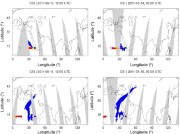
Figure 2.Unit simulation for the Nabro case study with air parcels initialized around 13 June, 00:00 UTC and 16.5 km altitude. The CSI analysis is performed on a 1◦×1◦longitude–latitude grid. Gray color indicates missing satellite data. Orange color corresponds to positive model forecasts, but lack of satellite data. Yellow color in-dicates positive forecasts and positive satellite observations. Blue color corresponds to negative forecasts with positive observations. Red color corresponds to positive forecasts with negative observa-tions. The black square shows the location of the Nabro volcano.
results are used to test the data match in grid boxes. SO2 col-umn densities are not compared directly. As mentioned ear-lier, the analysis is performed on a 1◦×1◦longitude–latitude grid.
Based on these examples, the unit simulations can be clas-sified into three categories. In the first category, we con-sider the cases in which the assigned initialization in the spe-cific subdomain yields SO2air parcel trajectories that match the satellite observations well. As an example, Fig. 2 shows the unit simulation with an initialization of emissions on 13 June 2011, 00:00 UTC±30 min and at(16.5±0.125)km altitude. This simulation shows excellent agreement with parts of the satellite observations over the entire simulation time period. This indicates that SO2 emissions most likely occurred in the corresponding temporal and spatial subdo-main.
In the second category, we consider the cases where model forecasts quickly mismatch the satellite observations. As an example, Fig. 3 shows a model forecast related to emis-sions released at the same time as in the first example, but at(29±0.125)km altitude. Figure 3 illustrates that the fore-casts agree with the satellite observations only shortly after the volcanic eruption. After 12 h the SO2air parcels were al-ready transported westwards, not agreeing with the satellite observations. Hence, this indicates that SO2emissions were not likely to occur in this temporal and spatial subdomain.
Figure 3.Same as Fig. 2, but for a unit simulation initialized at 29 km altitude. This simulation almost immediately disagrees with the satellite observations. Note that the time steps are partly differ-ent from those shown in Fig. 2.
Figure 4.Same as Fig. 2, but for a unit simulation initialized at 20 km altitude. This simulation agrees with the satellite observa-tions for about 48 h, but disagrees at later times. Note that the time steps are partly different from those shown in Figs. 2 and 3.
In the third category, successful model forecasts can be found for a longer time period compared with second cat-egory. The example presented in Fig. 4, with air parcels re-leased at the same time but at(20±0.125)km altitude, shows agreement between the model forecast and the satellite obser-vations for about 2 days. However, the SO2air parcels were transported westwards and are not agreeing with the satellite observations at later times. Also in this temporal and spatial subdomain SO2emissions were not likely to occur.
As will be shown in the subsequent sections, both the mean rule and the product rule work well for the cases in the first category. They can therefore capture the basic transport dy-namics. However, for less realistic situations in the second and third category the application of the mean rule still yields small importance weights. The product rule can be used to exclude these unrealistic cases and yield proper importance weights by choosing a suitable split point of the obtained CSI time series. As will be shown in Sect. 4.6, it is therefore con-sidered as a superior strategy, both qualitatively and quanti-tatively.
4.3 Reconstruction of volcanic SO2emissions
Suitable initializations are necessary in order to perform re-liable final forward simulations. For this purpose we esti-mate the time- and altitude-dependent volcanic SO2 emis-sions with the iterative inversion approach outlined in Sect. 3. The time- and altitude-resolved emission rates are estimated based on the different weight-updating schemes. By assum-ing a total mass of 1.5×10⁹kg for the entire initialization do-main, the equal-probability resampling strategy (first guess) considers an equal weight of wij=1/15 840 that leads to
constant and vertically uniform emission rates of approxi-mately 0.1052 kg m−1s−1. However, note that such an as-sumption is in general not very realistic, even by posing fur-ther time- and altitude-constraints, because volcanic erup-tions often change over time significantly and emissions are also not uniformly distributed with altitude.
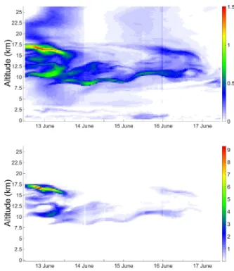
Figure 5 shows the temporally and spatially resolved SO2emission rates reconstructed by applying the mean rule and the product rule, respectively. The application of the mean rule results in temporally and spatially broader ar-eas with smaller emission rates (Fig. 5, top) up to about 1.5 kg m−1s−1. As shown in the figure, some unlikely cases of local emissions mentioned in Sect. 4.2 are not excluded. In contrast, the application of the product rule emphasizes the more likely cases and excludes unlikely cases (Fig. 5, bottom). Its maximum emission rate is about 6 times larger than that of the mean rule. In particular, the peak emission rates on 13 June 2011, 00:00 UTC, 14 June 2011, 15:00 UTC, and 16 June 2011, 10:00 UTC are approximately 9.28, 0.57, and 0.70 kg m−1s−1, respectively. The corresponding peak emission rates estimated by the mean rule are approximately 1.50, 0.56, and 0.42 kg m−1s−1. Since the total emission con-sidered in this study (1.5×10⁹kg) is the same for all emis-sion reconstruction schemes, and the mean rule yields some local emissions for unlikely cases (for instance at altitudes above 20 km), the emissions for more likely cases (e. g., on 13 June 2011, 00:00 UTC at 16.5 km altitude) are underesti-mated.
Our results qualitatively agree with the emission data re-constructed by the backward-trajectory approach presented by Hoffmann et al. (2016). The maximum emission rates ob-tained by the backward-trajectory approach are in between
Figure 5.Reconstructed SO2emission rates (kg m−1s−1) for the
Nabro eruption in June 2011. Emission rates were obtained by ap-plying the mean rule (top) and the product rule (bottom) weight-updating schemes of the proposed inversion approach (see text for details).
the maximum values obtained with the mean rule and the product rule weight-updating schemes used here. Even closer agreement with the backward-trajectory approach might be achieved by tuning the split point of the product rule accord-ingly. A sensitivity study for this important tuning parameter will be presented in Sect. 4.4. As shown in Fig. 5, the recon-structed emissions contain very low oscillations, which indi-cates that the estimations are well constrained by the avail-able AIRS satellite data.
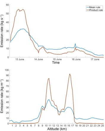
Finally, Fig. 6 shows the reconstructed emission rates in-tegrated over time and altitude. As found earlier, the max-imum emission rates for the main eruption on 13 June ob-tained by the product rule are much higher (up to a factor of 2 for the integrated values) than those obtained by the mean rule. However, this is compensated by lower emission rates by the product rule from 14 to 17 June. Considering the al-titude distribution, Fig. 6 (bottom) reveals, especially for the product rule, that most SO2emissions occurred at 10 to 12 and 15 to 17 km altitude. We find that the altitude distribution is less constrained for the mean rule than for the product rule. 4.4 Sensitivity analysis for the weight-updating
schemes
In this section, we first discuss the effect of different choices of the parameter nk for the mean rule weight-updating
num-Figure 6. Comparison of reconstructed emission rates integrated over altitude (top) and time (bottom) for the mean rule and the prod-uct rule weight-updating schemes.
ber of discrete-time intervals used for the CSI analysis. It di-rectly corresponds to the choice of the final time step of the satellite data. For the reference simulations we have chosen 23 June 2011, 00:00 UTC as the final time, corresponding to nk=21. Figure 7 (top) displays a contour plot of the
impor-tance weights for the reference case. Figure 7 (middle and bottom) shows the absolute differences with respect to other final times. By choosing 22 June 2011, 00:00 UTC (nk=19)
and 24 June 2011, 00:00 UTC (nk=23) as the final times,
the relative differences of the importance weights are about 9.5 and 10 %, respectively. The choice of 22 June 2011, 12:00 UTC (nk=20) and 23 June 2011, 12:00 UTC (nk=
22) as final time lead to smaller relative differences, about 7.2 and 6.2 %, respectively (not shown). Based on a visual inspection, the aforementioned different importance weights all show rather similar results in the final forward simula-tions.
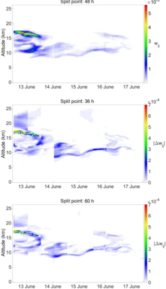
For the product rule, we performed a sensitivity analysis withnk corresponding to the reference date (23 June 2011,
00:00 UTC), but we choose five different split pointsn′k, cor-responding to 24, 36, 48, 60, and 72 h after the beginning of the simulation (13 June 2011, 00:00 UTC). Considering 48 h as the reference case, the choice of the other split points lead to 23.1, 11.3, 8.7, and 13.7 % relative differences of the im-portance weights. Except in the case of 24 h, which is too short to constrain the time and altitude distribution of the
Figure 7.Sensitivity analysis for the mean rule parameternk:
esti-mated importance weightswijfor choosing 23 June, 00:00 UTC as
the final time of used satellite data (top); absolute differences of esti-mated importance weights|1wij|for choosing 23 June, 00:00 UTC as the final time and those for choosing 22 June, 00:00 UTC (mid-dle) and 24 June, 00:00 UTC (bottom) as final time.
Figure 8.Sensitivity analysis for the product rule parametern′k: es-timated importance weightswijfor choosing 23 June 00:00 as the
final time of used satellite data and 48 h as the split point (top); abso-lute differences of estimated importance weights|1wij|for
choos-ing 48 h as the split point and those for chooschoos-ing 36 h (middle) and 60 h (bottom) as split point.
4.5 Validation of emission time series
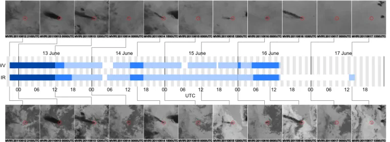
From MVIRI WV and IR measurements aboard Meteosat-7 (IODC) (Fig. 9, top and bottom panel), we derived time se-ries information (Fig. 9, middle panel) of the eruption his-tory. The WV channel gives information on the high alti-tude eruption phase because it gets optically thick in the middle troposphere (around 6 km), where also the AIRS SO2 channel gets optically thick. In contrast, the IR chan-nel reaches down to the ground and also gives information on low altitude plumes (e.g., on 17 June 2011). The satel-lite imagery indicates that the strongest eruptions occurred between 13 June 2011, 00:00 and 12:00 UTC. A series of smaller emission events until 16 June 2011, 15:00 UTC were also observed. In particular, there were two short-time
peri-ods of strong eruptions on 14 and 16 June 2011. The emission time series derived with our inverse modeling approach are in good temporal agreement with the MVIRI observations.
Injection altitudes of the Nabro eruption have been dis-cussed recently, mostly based on different satellite measure-ments (Bourassa et al., 2012; Fromm et al., 2013; Vernier et al., 2013; Fromm et al., 2014). For the evaluation of the SO2heights we used MIPAS and CALIOP H2SO4(sulfate aerosol) detections. This aerosol forms from the SO2 and hence, it can be seen as an indicator for the position of the SO2. As other studies already found (Fromm et al., 2014; Clarisse et al., 2014) there was very little ash in the Nabro plume. However, to really make sure that we did not com-pare with ash, we checked the CALIOP depolarization ratio (no depolarization for liquid particles) and filtered out vol-canic ash using the MIPAS volvol-canic ash detection algorithm (Griessbach et al., 2014). The first CALIOP aerosol obser-vations found the initial plume at 11–15.5 km over Pakistan and at 15–16.5 km over Iran on 15 June. Plumes were mea-sured at 18–19 and 8.5 –11.5 km over Egypt, at 16–17.5 km over Turkey, at 8.5–11 km over the Arabian Peninsula, at 16– 17 km over Iran, and at 14–16.2 km over China on 16 June. MIPAS detected the aerosol resulting from Nabro eruption at 12–16.5 km over Israel on 14 June. The aerosol layers nearest to the Nabro were measured at 11–16.5 km on 15 June. They reached 16–18.5 km on 16 June and 12–15.5 km on 17 June. The altitudes measured by CALIOP and MIPAS agree within their uncertainties.
13 June 14 June 15 June 16 June 17 June
00 06 12 18 00 06 12 18 00 06 12 18 00 06 12 18 00 06 12 18
UTC WV
IR
Figure 9.Time line of the 2011 Nabro eruption based on MVIRI IR and WV measurements from Meteosat-7 (IODC). The satellite images were used to roughly estimate the strength of the volcanic activity (white is none, light blue is low level, blue is medium level, dark blue is high level).
Figure 10.Comparison of the critical success index (CSI), the false alarm rate (FAR), and the probability of detection (POD) time series during 12 h time intervals obtained by applying the equal-probability strategy, the mean rule, and the product rule.
4.6 Final forward simulations
We performed the final forward simulations for the Nabro case study with the initializations obtained in Sect. 4.3. Fig-ure 10 shows the corresponding CSI, POD, and FAR time series based on 12 h time intervals, obtained by applying the equal-probability strategy, the mean rule, and the prod-uct rule, respectively. Note that the equal-probability strat-egy assumes a constant emission rate in the entire time-and altitude-dependent initialization domain. In all cases, the
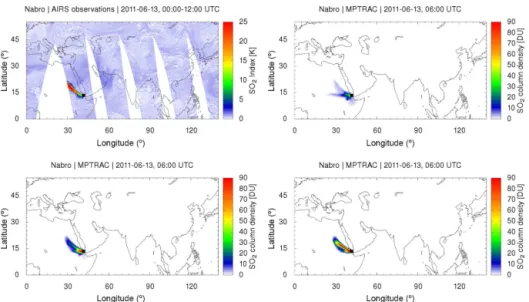
Figure 11.Comparison of AIRS satellite observations (top, left) and MPTRAC simulation results on 13 June 2011, 06:00 UTC based on the equal-probability strategy (top, right), the mean rule (bottom, left), and the product rule (bottom, right).
Figure 12.Same as Fig. 11, but for 14 June 2011, 06:00 UTC.
application of the product rule provides the best simulation results of all three cases. Its maximum and mean CSI val-ues are 52.4 and 21.4 %, respectively. Our findings for the CSI are confirmed by the FAR and POD time series (Fig. 10, lower panels), which indicates that the use of product rule yields the best simulation results of the three cases.
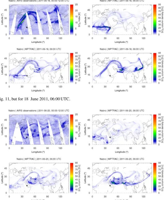
Figures 11 to 17 compare the simulation results with AIRS satellite observations for selected time steps. SO2 column densities from the model are presented on a 0.5◦×0.5◦ longitude–latitude grid. The AIRS SO2index during corre-sponding 12 h time periods is presented on the measurement grid of the instrument. In the case of the equal-probability strategy, unrealistic transport of air parcels westward of the Nabro is found. Accordingly, the estimated SO2column
den-sities for realistic pathways are significantly lower. In the case of the mean rule, more realistic forecasts of the basic SO2transport patterns are obtained. The simulation results are qualitatively closer to the satellite observations both in time and space. However, unrealistic westward transport of SO2is still recognizable. The product rule clearly yields the most reliable simulation results of the three cases. It most successfully excludes unlikely local emission patterns.
Figure 13.Same as Fig. 11, but for 15 June 2011, 06:00 UTC.
Figure 14.Same as Fig. 11, but for 16 June 2011, 06:00 UTC.
to the GOME-2 satellite retrievals reported by Theys et al. (2013, Fig. 10b–d). Our simulations (Figs. 12 and 14) show more realistic transport patterns on 14 and 16 June 2011 than the FLEXPART model outputs based on the IASI data (Theys et al., 2013, Fig. 12). Besides, the SO2 distributions on 16 and 18 June 2011 in China are not well captured by the FLEXPART model outputs based on the GOME-2 data (Theys et al., 2013, Fig. 10b and c), but by our simulations (Figs. 14 and 15). Furthermore, the SO2 transport patterns of our simulations are in good agreement with IASI obser-vations that were extensively studied in the context of the Nabro eruption (Clarisse et al., 2014, Figs. 6–10).
5 Conclusions and outlook
ini-Figure 15.Same as Fig. 11, but for 18 June 2011, 06:00 UTC.
Figure 16.Same as Fig. 11, but for 20 June 2011, 06:00 UTC.
tialization domain, which is estimated by the proposed inver-sion algorithm, the local SO2emission rates can be obtained. Together with the equal-probability assumption, two weight-updating schemes, referred to as the mean rule and product rule have been proposed for the reconstruction of emission data. Considering the Nabro eruption in June 2011 as a case study, we qualitatively assessed the reconstructed emission time series by comparing them with Meteosat-7 (IODC) imagery to validate the temporal development and with CALIOP and MIPAS satellite observations to confirm the injection altitudes. Simulation results based on the initial-izations reconstructed by different weight-updating schemes have been compared, in particular, to demonstrate the advan-tages of the product rule. The mean and maximum CSI val-ues obtained by using the equal-probability strategy are 8.1
and 32.3 %, respectively. The mean rule yields a mean CSI value of 16.6 % and a maximum of 41.2 %. The product rule leads to an improvement of the mean CSI value to 21.4 % and of the maximum CSI value to 52.4 %. The simulation re-sults for the Nabro case study show good agreement with the AIRS satellite observations in terms of SO2horizontal distri-butions and have been validated through other independent data sets such as IASI and GOME-2 satellite observations re-ported by other studies. The simulation results show that the inverse modeling system successfully identified the complex volcanic emission pattern of the Nabro eruption, and helped to further reveal the complex transport processes through the Asian monsoon circulation.
Figure 17.Same as Fig. 11, but for 24 June 2011, 06:00 UTC.
of the current approach towards near-real-time forecasting, the development of an adaptive strategy for discretizing the initialization domain, the consideration of the SO2 kernel functions, and a detailed treatment of data uncertainties. An adaptive strategy is expected to reduce the computational ef-fort and to provide better resolution in areas of the initial-ization domain where there is large variability. This way, we would expect more precise importance weights estimated for the most likely cases of local emission and hence more ac-curate simulation results with better local details in a quan-titative manner. In particular, the SO2 kernel functions of the AIRS channels used to calculate the SI depend on atmo-spheric conditions and altitude (e.g., Hoffmann et al., 2016, Fig. 1). However, variations in the UT/LS region where most of the Nabro emissions occurred are not too large. Hence, we did not consider this dependency in our analysis. How-ever, the consideration of the AIRS kernel functions in the CSI analysis will be an important aspect in future work. Un-certainties in the meteorological data are another important source of error. The topic is addressed in a recent study by Hoffmann et al. (2016), wherein four different meteorologi-cal products have been tested for the MPTRAC simulations. This work aims to introduce an inversion approach for SO2 transport simulations. A more detailed, quantitative study of the errors resulting from the uncertainties of different mete-orological data will be considered in future work. Further-more, the version of MPTRAC used in this study did not consider loss processes of SO2. Hoffmann et al. (2016) used a newer version of MPTRAC, which takes into account loss processes of SO2. Although the simulation results by means of the two different versions of MPTRAC are rather similar, a precise quantitative analysis considering the SO2loss will be subject of future efforts. Further research shall also be de-voted to the testing of the proposed MPTRAC-based inverse
modeling and simulation system for other case studies of vol-canic eruptions and its capacity for forecasting.
Code and data availability
The current release of the MPTRAC model can be down-loaded from the model web site at http://www.fz-juelich.de/ ias/jsc/mptrac. The code version used in this study can be obtained by contacting the corresponding author. The time-and altitude-dependent emission time series obtained with the different weight-updating schemes (Fig. 5) are provided as an electronic supplement to this paper. This allows our results to be reproduced and extended in future work, for in-stance by performing simulations with other transport mod-els.
The Supplement related to this article is available online at doi:10.5194/gmd-9-1627-2016-supplement.
Acknowledgements. AIRS data products were obtained from the NASA Goddard Earth Sciences Data Information and Services Center (GES DISC). ERA-Interim data were obtained from the European Centre for Medium-Range Weather Forecasts (ECMWF). The authors gratefully acknowledge the computing time granted on the supercomputer JuRoPA at the Jülich Supercomputing Centre (JSC).
The article processing charges for this open-access publication were covered by a Research
References
Aumann, H. H., Chahine, M. T., Gautier, C., Goldberg, M. D., Kalnay, E., McMillin, L. M., Revercomb, H., Rosenkranz, P. W., Smith, W. L., Staelin, D. H., Strow, L. L., and Susskind, J.: AIRS/AMSU/HSB on the Aqua Mission: design, science objec-tives, data products, and processing systems, IEEE T. Geosci. Remote, 41, 253–264, 2003.
Bourassa, A. E., Robock, A., Randel, W. J., Deshler, T., Rieger, L. A., Lloyd, N. D., Llewellyn, E. J. T., and Degen-stein, D. A.: Large Volcanic Aerosol Load in the Stratosphere Linked to Asian Monsoon Transport, Science, 337, 78–81, 2012. Brenot, H., Theys, N., Clarisse, L., van Geffen, J., van Gent, J., Van Roozendael, M., van der A, R., Hurtmans, D., Coheur, P.-F., Clerbaux, C., Valks, P., Hedelt, P., Prata, F., Rasson, O., Sievers, K., and Zehner, C.: Support to Aviation Control Service (SACS): an online service for near-real-time satellite monitoring of vol-canic plumes, Nat. Hazards Earth Syst. Sci., 14, 1099–1123, doi:10.5194/nhess-14-1099-2014, 2014.
Carn, S. A., Krueger, A. J., Krotkov, N. A., Yang, K., and Evans, K.: Tracking volcanic sulfur dioxide clouds for aviation hazard mit-igation, Nat. Hazards, 51, 325–343, 2009.
Casadevall, T. J.: The 1989–1990 eruption of Redoubt Volcano, Alaska: impacts on aircraft operations, J. Volcanol. Geoth. Res., 62, 301–316, 1994.
Chahine, M. T., Pagano, T. S., Aumann, H. H., Atlas, R., Bar-net, C., Blaisdell, J., Chen, L., Divakarla, M., Fetzer, E. J., Gold-berg, M., Gautier, C., Granger, S., Hannon, S., Irion, F. W., Kakar, R., Kalnay, E., Lambrigtsen, B. H., Lee, S., Mar-shall, J. L., McMillan, W. W., McMillin, L., Olsen, E. T., Rever-comb, H., Rosenkranz, P., Smith, W. L., Staelin, D., Strow, L. L., Susskind, J., Tobin, D., Wolf, W., and Zhou, L.: AIRS: improv-ing weather forecastimprov-ing and providimprov-ing new data on greenhouse gases, B. Am. Meteorol. Soc., 87, 911–926, 2006.
Clarisse, L., R’Honi, Y., Coheur, P.-F., Hurtmans, D., and Clerbaux, C.: Thermal infrared nadir observations of 24 atmospheric gases, Geophys. Res. Lett., 38, L10802, doi:10.1029/2011GL047271, 2011.
Clarisse, L., Hurtmans, D., Clerbaux, C., Hadji-Lazaro, J., Ngadi, Y., and Coheur, P.-F.: Retrieval of sulphur dioxide from the infrared atmospheric sounding interferometer (IASI), Atmos. Meas. Tech., 5, 581–594, doi:10.5194/amt-5-581-2012, 2012. Clarisse, L., Coheur, P.-F., Prata, F., Hadji-Lazaro, J., Hurtmans, D.,
and Clerbaux, C.: A unified approach to infrared aerosol remote sensing and type specification, Atmos. Chem. Phys., 13, 2195– 2221, doi:10.5194/acp-13-2195-2013, 2013.
Clarisse, L., Coheur, P.-F., Theys, N., Hurtmans, D., and Clerbaux, C.: The 2011 Nabro eruption, a SO2plume height analysis
us-ing IASI measurements, Atmos. Chem. Phys., 14, 3095–3111, doi:10.5194/acp-14-3095-2014, 2014.
Clerbaux, C., Boynard, A., Clarisse, L., George, M., Hadji-Lazaro, J., Herbin, H., Hurtmans, D., Pommier, M., Razavi, A., Turquety, S., Wespes, C., and Coheur, P.-F.: Monitoring of atmospheric composition using the thermal infrared IASI/MetOp sounder, At-mos. Chem. Phys., 9, 6041–6054, doi:10.5194/acp-9-6041-2009, 2009.
Dee, D. P., Uppala, S. M., Simmons, A. J., Berrisford, P., Poli, P., Kobayashi, S., Andrae, U., Balmaseda, M. A., Balsamo, G., Bauer, P., Bechtold, P., Beljaars, A. C. M., van de Berg, L., Bidlot, J., Bormann, N., Delsol, C., Dragani, R., Fuentes, M.,
Geer, A. J., Haimberger, L., Healy, S. B., Hersbach, H., Hólm, E. V., Isaksen, L., Kãllberg, P., Köhler, M., Matricardi, M., McNally, A. P., Monge-Sanz, B. M., Morcrette, J.-J., Park, B.-K., Peubey, C., de Rosnay, P., Tavolato, C., Thépaut, J.-N., and Vitart, F.: The ERA-Interim reanalysis: configuration and perfor-mance of the data assimilation system, Q. J. Roy. Meteor. Soc., 137, 553–597, 2011.
Del Moral, P.: Non Linear Filtering: Interacting Particle Solution, Markov Processes and Related Fields, 2, 555–580, 1996. Draxler, R. R. and Hess, G. D.: An overview of the HYSPLIT_4
modeling system of trajectories, dispersion, and deposition, Aust. Meteorol. Mag., 47, 295–308, 1998.
Eckhardt, S., Prata, A. J., Seibert, P., Stebel, K., and Stohl, A.: Esti-mation of the vertical profile of sulfur dioxide injection into the atmosphere by a volcanic eruption using satellite column mea-surements and inverse transport modeling, Atmos. Chem. Phys., 8, 3881–3897, doi:10.5194/acp-8-3881-2008, 2008.
Fischer, H., Birk, M., Blom, C., Carli, B., Carlotti, M., von Clar-mann, T., Delbouille, L., Dudhia, A., Ehhalt, D., EndeClar-mann, M., Flaud, J. M., Gessner, R., Kleinert, A., Koopman, R., Langen, J., López-Puertas, M., Mosner, P., Nett, H., Oelhaf, H., Perron, G., Remedios, J., Ridolfi, M., Stiller, G., and Zander, R.: MIPAS: an instrument for atmospheric and climate research, Atmos. Chem. Phys., 8, 2151–2188, doi:10.5194/acp-8-2151-2008, 2008. Flemming, J. and Inness, A.: Volcanic sulfur dioxide plume
fore-casts based on UV satellite retrievals for the 2011 Grímsvötn and the 2010 Eyjafjallajökull eruption, J. Geophys. Res., 118, 10172– 10189, 2013.
Fromm, M., Nedoluha, G., and Charvát, Z.: Comment on “Large Volcanic Aerosol Load in the Stratosphere Linked to Asian Monsoon Transport”, Science, 339, p. 647, doi:10.1126/science.1228605, 2013.
Fromm, M., Kablick III, G., Nedoluha, G., Carboni, E., Grainger, R., Campbell, J., and Lewis, J.: Correcting the record of volcanic stratospheric aerosol impact: Nabro and Sarychev Peak, J. Geophys. Res., 119, 10343–10364, 2014.
Gordon, N. J., Salmond, D. J., and Smith, A. F. M.: Novel approach to nonlinear/non-Gaussian Bayesian state estimation, IEE Pro-ceedings F (Radar and Signal Processing), 140, 107–113, 1993. Griessbach, S., Hoffmann, L., von Hobe, M., Müller, R., Spang, R.
and Riese, M.: A six-year record of volcanic ash detection with Envisat MIPAS, in: Proceedings of ESA ATMOS 2012, Eu-ropean Space Agency, ESA Special Publication SP-708 (CD-ROM), 2012.
Griessbach, S., Hoffmann, L., Spang, R., and Riese, M.: Volcanic ash detection with infrared limb sounding: MIPAS observations and radiative transfer simulations, Atmos. Meas. Tech., 7, 1487– 1507, doi:10.5194/amt-7-1487-2014, 2014.
Griessbach, S., Hoffmann, L., Spang, R., von Hobe, M., Müller, R., and Riese, M.: Infrared limb emission measurements of aerosol in the troposphere and stratosphere, Atmos. Meas. Tech. Dis-cuss., 8, 4379–4412, doi:10.5194/amtd-8-4379-2015, 2015. Harvey, N. J. and Dacre, H. F.: Spatial evaluation of volcanic ash
forecasts using satellite observations, Atmos. Chem. Phys., 16, 861–872, doi:10.5194/acp-16-861-2016, 2016.
Guidard, V., Hurtmans, D., Illingworth, S., Jacquinet-Husson, N., Kerzenmacher, T., Klaes, D., Lavanant, L., Masiello, G., Ma-tricardi, M., McNally, A., Newman, S., Pavelin, E., Payan, S., Péquignot, E., Peyridieu, S., Phulpin, T., Remedios, J., Schlüs-sel, P., Serio, C., Strow, L., Stubenrauch, C., Taylor, J., Tobin, D., Wolf, W., and Zhou, D.: Hyperspectral Earth Observation from IASI: Five Years of Accomplishments, Bull. Amer. Meteor. Soc., 93, 347–370, 2012.
Hoffmann, L. and Alexander, M. J.: Retrieval of stratospheric tem-peratures from Atmospheric Infrared Sounder radiance measure-ments for gravity wave studies, J. Geophys. Res., 114, D07105, doi:10.1029/2008JD011241, 2009.
Hoffmann, L. and Alexander, M. J.: Occurrence frequency of convective gravity waves during the North Ameri-can thunderstorm season, J. Geophys. Res., 115, D20111, doi:10.1029/2010JD014401, 2010.
Hoffmann, L., Griessbach, S., and Meyer, C. I.: Volcanic emis-sions from AIRS observations: detection methods, case study, and statistical analysis, Proc. SPIE, 9242, 924214–924214-8, doi:10.1117/12.2066326, 2014.
Hoffmann, L., Rößler, T., Griessbach, S., Heng, Y., and Stein, O.: Lagrangian transport simulations of volcanic sulfur dioxide emissions: impact of meteorological data products, J. Geophys. Res.-Atmos., 121, doi:10.1002/2015JD023749, 2016.
Jones, A., Thomson, D., Hort, M., and Devenish, B.: Volcanic emissions from AIRS observations: The UK Met Office’s next-generation atmospheric dispersion model, NAME III, in Air Pol-lution Modeling and its Application XVII, 580–589, Springer, 2007.
Karagulian, F., Clarisse, L., Clerbaux, C., Prata, A. J., Hurt-mans, D., and Coheur, P. F.: Detection of volcanic SO2,
ash, and H2SO4 using the Infrared Atmospheric
Sound-ing Interferometer (IASI), J. Geophys. Res., 115, D00L02, doi:10.1029/2009JD012786, 2010.
Kristiansen, N. I., Stohl, A., Prata, A. J., Bukowiecki, N., Dacre, H., Eckhardt, S., Henne, S., Hort, M. C., Johnson, B. T., Marenco, F., Neininger, B., Reitebuch, O., Seibert, P., Thomson, D. J., Web-ster, H. N., and Weinzierl, B.: Performance assessment of a vol-canic ash transport model mini-ensemble used for inverse model-ing of the 2010 Eyjafjallajökull eruption, J. Geophys. Res., 117, D00U11, doi:10.1029/2011JD016844, 2012.
Kristiansen, N. I., Prata, A. J., Stohl, A., and Carn, S. A.: Strato-spheric volcanic ash emissions from the 13 February 2014 Kelut eruption, Geophys. Res. Lett., 42, 588–596, 2015.
Lacasse, C., Karlsdóttir, S., Larsen, G., Soosalu, H., Rose, W., and Ernst, G.: Weather radar observations of the Hekla 2000 eruption cloud, Iceland, B. Volcanol., 66, 457–473, 2004.
Lamb, H. H.: Volcanic dust in the atmosphere, with a chronology and assessment of its meteorological significance, Philos. T. Roy. Soc. A, 266, 425–533, 1970.
Moxnes, E. D., Kristiansen, N. I., Stohl, A., Clarisse, L., Durant, A., Weber, K., and Vogel, A.: Separation of ash and sulfur diox-ide during the 2011 Grímsvötn eruption, J. Geophys. Res., 119, 7477–7501, doi:10.1002/2013JD021129, 2014.
Munro, R., Eisinger, M., Anderson, C., Callies, J., Corpaccioli, E., Lang, R., Lefebvre, A., Livschitz, Y., and Albinana, A. P.: GOME-2 on MetOp, in: Proceedings of The 2006 EUMET-SAT Meteorological Satellite Conference, Helsinki, Finland, 12– 16 June 2006, EUMETSAT p. 48, 2006.
Prata, A. J.: Satellite detection of hazardous volcanic clouds and the risk to global air traffic, Nat. Hazards, 51, 303–324, 2009. Raspollini, P., Carli, B., Carlotti, M., Ceccherini, S., Dehn, A.,
Dinelli, B. M., Dudhia, A., Flaud, J.-M., López-Puertas, M., Niro, F., Remedios, J. J., Ridolfi, M., Sembhi, H., Sgheri, L., and von Clarmann, T.: Ten years of MIPAS measurements with ESA Level 2 processor V6 – Part 1: Retrieval algorithm and di-agnostics of the products, Atmos. Meas. Tech., 6, 2419–2439, doi:10.5194/amt-6-2419-2013, 2013.
Robock, A.: Volcanic eruptions and climate, Rev. Geophys., 38, 191–219, 2000.
Schaefer, J. T.: The critical success index as an indicator of warning skill, Weather Forecast., 5, 570–575, 1990.
Sears, T. M., Thomas, G. E., Carboni, E. A., Smith, A. J., and Grainger, R. G.: SO2as a possible proxy for volcanic ash in
avia-tion hazard avoidance, J. Geophys. Res., 118, 5698–5709, 2013. Seibert, P.: Inverse modelling of sulfur emissions in Europe based on trajectories, in: Inverse Methods in Global Biogeochemical Cycles, edited by: Kasibhatla, P., Heimann, M., Rayner, P., Ma-howald, N., Prinn, R. G., and Hartley, D. E., Geophysical Mono-graph 114, American Geophysical Union, ISBN-10: 0-87590-097-6, Washington DC, USA, 147–154, 2000.
Solomon, S., Daniel, J. S., Neely, R., Vernier, J.-P., Dutton, E. G., and Thomason, L. W.: The persistently variable “background” stratospheric aerosol layer and global climate change, Science, 333, 866–870, 2011.
Stein, O., Flemming, J., Inness, A., Kaiser, J. W., and Schultz, M. G.: Global reactive gases forecasts and reanalysis in the MACC project, J. Integr. Environ. Sci., 9, 57–70, 2012. Stohl, A., Forster, C., Frank, A., Seibert, P., and Wotawa, G.:
Technical note: The Lagrangian particle dispersion model FLEXPART version 6.2, Atmos. Chem. Phys., 5, 2461–2474, doi:10.5194/acp-5-2461-2005, 2005.
Stohl, A., Prata, A. J., Eckhardt, S., Clarisse, L., Durant, A., Henne, S., Kristiansen, N. I., Minikin, A., Schumann, U., Seibert, P., Stebel, K., Thomas, H. E., Thorsteinsson, T., Tørseth, K., and Weinzierl, B.: Determination of time- and height-resolved vol-canic ash emissions and their use for quantitative ash disper-sion modeling: the 2010 Eyjafjallajökull eruption, Atmos. Chem. Phys., 11, 4333–4351, doi:10.5194/acp-11-4333-2011, 2011. Stunder, B. J., Heffter, J. L., and Draxler, R. R.: Airborne volcanic
ash forecast area reliability, Weath. Forecast, 22, 1132–1139, 2007.
Theys, N., Campion, R., Clarisse, L., Brenot, H., van Gent, J., Dils, B., Corradini, S., Merucci, L., Coheur, P.-F., Van Roozendael, M., Hurtmans, D., Clerbaux, C., Tait, S., and Ferrucci, F.: Vol-canic SO2fluxes derived from satellite data: a survey using OMI,
GOME-2, IASI and MODIS, Atmos. Chem. Phys., 13, 5945– 5968, doi:10.5194/acp-13-5945-2013, 2013.
Tikhonov, A. N. and Arsenin, V. Y.: Solutions of Ill-posed Prob-lems, V. H. Winston and Sons, Washington, ISBN-10: 0-470-99124-0, 1977.
Webley, P., Stunder, B., and Dean, K.: Preliminary sensitivity study of eruption source parameters for operational volcanic ash cloud transport and dispersion models – a case study of the August 1992 eruption of the Crater Peak vent, Mount Spurr, Alaska, J. Volcanol. Geotherm. Res., 186, 108–119, 2009.
Wernli, H. and Davies, H. C.: A Lagrangian-based analysis of ex-tratropical cyclones, I: The method and some applications, Q. J. Roy. Meteor. Soc., 123, 467–489, 1997.