www.atmos-chem-phys.net/14/4779/2014/ doi:10.5194/acp-14-4779-2014
© Author(s) 2014. CC Attribution 3.0 License.
Atmospheric
Chemistry
and Physics
Sulfur hexafluoride (SF
6
) emissions in East Asia determined by
inverse modeling
X. Fang1,2, R. L. Thompson1, T. Saito3, Y. Yokouchi3, J. Kim4,5, S. Li4,6, K. R. Kim4,6, S. Park7, F. Graziosi8, and A. Stohl1
1Norwegian Institute for Air Research, Kjeller, Norway
2State Key Joint Laboratory for Environmental Simulation and Pollution Control, College of Environmental Sciences and
Engineering, Peking University, Beijing, China
3National Institute for Environmental Studies, Tsukuba, Japan
4School of Earth and Environmental Sciences, Seoul National University, Seoul, South Korea
5Scripps Institution of Oceanography, University of California at San Diego, La Jolla, California, USA 6Research Institute of Oceanography, Seoul National University, Seoul, South Korea
7Department of Oceanography, Kyungpook National University, Sangju, South Korea 8University of Urbino, Urbino, Italy
Correspondence to:X. Fang ([email protected])
Received: 4 June 2013 – Published in Atmos. Chem. Phys. Discuss.: 13 August 2013 Revised: 11 March 2014 – Accepted: 20 March 2014 – Published: 14 May 2014
Abstract. Sulfur hexafluoride (SF6)has a global warming
potential of around 22 800 over a 100-year time horizon and is one of the greenhouse gases regulated under the Kyoto Protocol. Around the year 2000 there was a reversal in the global SF6emission trend, from a decreasing to an
increas-ing trend, which was likely caused by increasincreas-ing emissions in countries that are not obligated to report their annual emis-sions to the United Nations Framework Convention on Cli-mate Change. In this study, SF6emissions during the period
2006–2012 for all East Asian countries – including Mongo-lia, China, Taiwan, North Korea, South Korea and Japan – were determined by using inverse modeling and in situ at-mospheric measurements. We found that the most impor-tant sources of uncertainty associated with these inversions are related to the choice of a priori emissions and their as-sumed uncertainty, the station network as well as the me-teorological input data. Much lower uncertainties are due to seasonal variability in the emissions, inversion geome-try and resolution, and the measurement calibration scale. Based on the results of these sensitivity tests, we estimate that the total SF6 emission in East Asia increased rapidly
from 2404±325 Mg yr−1in 2006 to 3787±512 Mg yr−1in 2009 and stabilized thereafter. China contributed 60–72 % to the total East Asian emission for the different years, followed
by South Korea (8–16 %), Japan (5–16 %) and Taiwan (4– 7 %), while the contributions from North Korea and Mongo-lia together were less than 3 % of the total. The per capita SF6emissions are highest in South Korea and Taiwan, while
the per capita emissions for China, North Korea and Japan are close to global average. During the period 2006–2012, emissions from China and from South Korea increased, while emissions from Taiwan and Japan decreased overall.
1 Introduction
Sulfur hexafluoride (SF6) is one of the greenhouse gases
(GHG) regulated under the Kyoto Protocol (UN, 1998). Its atmospheric lifetime is estimated to be∼3200 years (Rav-ishankara et al., 1993). It is the most potent GHG, with a global warming potential (GWP) of 22800 over a 100-year time horizon (Forster et al., 2007). The major source for SF6
to the atmosphere is fugitive emissions from high-voltage electric equipment, while the minor sources are magnesium production, electronics manufacturing, SF6 production and
2000, after a small decrease in the period 1995–2000 (Rigby et al., 2010). An explanation for this behavior is that SF6
emission reductions have been achieved in most of the de-veloped countries that are obligated to report their annual emissions to the United Nations Framework Convention on Climate Change (UNFCCC; so-called “Annex-I” countries). However, further emission reductions after the year 2000 could no longer compensate for the increase in the emissions from countries not required to report their emissions due to their developing status (so-called “non-Annex-1” countries; Levin et al., 2010; Rigby et al., 2010).
With the exception of Japan, all countries in East Asia – Mongolia, China, Taiwan, North Korea and South Korea – are non-Annex-I countries. Every year, the Greenhouse Gas Inventory Office of Japan (GIO) submits their emis-sion estimates based on inventory technology to the UN-FCCC (GIO, 2012). The second national communication of South Korea submitted to UNFCC reports SF6emissions of
around 700 Mg yr−1during the period 2006–2009 (Republic of Korea, 2012). The Second Communication for Taiwan re-ports SF6emissions of about 120 Mg yr−1within 2006–2008
(Taiwan, 2011). Mongolia and China only report emissions for 2005 of 0 Mg yr−1(Mongolia, 2010) and 436.7 Mg yr−1 (China, 2012), respectively. SF6emissions are not included
in North Korea’s Communication (Democratic People’s Re-public of Korea, 2000). These bottom-up national estimates, however, are uncertain and need independent validation.
Top-down estimates based on atmospheric SF6
measure-ments provide one way to validate these inventories. Based on measurements from the Shangdianzi station in China and a Lagrangian transport model, SF6 emissions from
China were estimated for the first time to be 800 (530– 1100) Mg yr−1 in October 2006–March 2008 (Vollmer et al., 2009). SF6 emissions were estimated for South Korea,
China and Japan during November 2007 to December 2008 based on an interspecies ratio method and atmospheric mea-surements at the Gosan station in South Korea (Li et al., 2011; Kim et al., 2010). Using combined Eulerian and La-grangian chemical transport models and measurement data from Gosan, average emissions for the period 2007–2009 were estimated for South Korea, China, Japan and Taiwan (Rigby et al., 2011). In some cases, discrepancies are found among these top-down estimates and the bottom-up invento-ries. For example, emissions from South Korea for 2008 were estimated to be 380 (330–440) Mg yr−1(Li et al., 2011), 221 (154–287) Mg yr−1(2007–2009 average, Rigby et al., 2011) and 728 Mg yr−1(Republic of Korea, 2012).
In this study, we quantify the emissions in East Asia dur-ing the last seven years (2006–2012) usdur-ing measurement data from several stations in this region, a Lagrangian particle dis-persion model, and inverse modeling.
2 Methodology 2.1 Measurement data
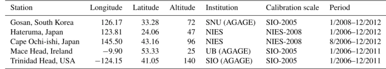
In this study, we used in situ measurements from three sta-tions in East Asia and from two stasta-tions outside East Asia (Table 1). The Asian stations are (1) Gosan, situated on Jeju Island in the Yellow Sea south of the Korean Peninsula and operated by Seoul National University (SNU), South Ko-rea (Kim et al., 2010), as part of the Advanced Global At-mospheric Gases Experiment (AGAGE) global network; (2) Hateruma, located on a small island with an area of 12.7 km2 at the southern edge of the Japanese archipelago; and (3) Cape Ochi-ishi, at the tip of the Nemuro Peninsula located in the eastern part of Hokkaido, Japan. Both Japanese sta-tions are operated by the National Institute for Environmental Studies (NIES; Tohjima et al., 2002).
At Gosan, ambient mixing ratios of SF6are measured
ev-ery two hours using the Medusa gas chromatograph–mass spectrometry (GC-MS) technology (Miller et al., 2008). Measurements of SF6 started in November 2007, but only
data from January 2008 were used here. At Hateruma and Cape Ochi-shi stations, SF6 mixing ratios are
mea-sured once per hour using a technique developed at NIES based on cryogenic preconcentration and a capillary GC-MS (Enomoto, 2005; Yokouchi et al., 2006). The Japanese measurements are reported on the NIES-2008 calibration scale, whereas for the other stations the SIO-2005 calibra-tion scale was used. Intercomparisons between the NIES-2008 and SIO-2005 scales yielded a NIES-NIES-2008 / SIO-2005 ratio of 1.013±0.006. We used this value to convert all NIES data from the NIES-2008 to the SIO-2005 calibration scale. Sensitivity tests demonstrate that using the NIES-2008 cali-bration scale as a reference increased the national emissions from all East Asian countries by less than 1.1 %, and that the differences in emissions were even smaller when SIO-2005-referenced data were adjusted to the widely used scale, NOAA-2006 (Hall et al., 2011), by multiplication by a con-stant factor of 1.002 derived from Rigby et al. (2010); there-fore, this will not be discussed any further.
Table 1.List of the measurement stations, corresponding coordinates, the operating institutions and the period of available data used in this study.
Station Longitude Latitude Altitude Institution Calibration scale Period
Gosan, South Korea 126.17 33.28 72 SNU (AGAGE) SIO-2005 1/2008–12/2012
Hateruma, Japan 123.81 24.06 47 NIES NIES-2008 1/2006–12/2012
Cape Ochi-ishi, Japan 145.50 43.16 96 NIES NIES-2008 8/2006–12/2012 Mace Head, Ireland −9.90 53.33 25 UB (AGAGE) SIO-2005 1/2006–12/2011 Trinidad Head, USA −124.15 41.05 140 SIO (AGAGE) SIO-2005 1/2006–12/2011
Fig. 1. Footprint emission sensitivity obtained from FLEXPART 20-day backward simulations based on ECMWF input data aver-aged for the period 2006–2012 for Gosan(a), Hateruma(b), Cape Ochi-shi(c)and all three stations(d). Black dots represent the cor-responding measurement stations.
2.2 Lagrangian backwards modeling
The method of Lagrangian backwards modeling used here is very similar to that presented in previous work (Stohl et al., 2009, 2010). Therefore, we only provide a brief de-scription of the method here. The Lagrangian particle dis-persion model FLEXPART v-9.02 (Stohl et al., 1998, 2005; http://www.flexpart.eu) was run every three hours for 20 days backwards in time to establish source–receptor relationships (SRR, often also called “footprints” or “emission sensitivi-ties”) between potential SF6emission sources and the change
in mixing ratio at each measurement station.
FLEXPART was driven by operational 3-hourly meteoro-logical data at 1◦×1◦resolution from the European Centre for Medium-Range Weather Forecasts (ECMWF) from 2006 to 2012. Figure 1 shows maps of average emission sensitiv-ities for each station as well as for all stations combined for the period 2006–2012. North Korea, South Korea, Japan, Tai-wan and the eastern part of China are well covered by the emission sensitivities of these three stations, which means
that influence of emissions from these countries should be seen in the measured mixing ratios. Western and southwest-ern China are not well covered; however, this region is only sparsely populated and emissions there are expected to be small. Therefore, the poor constraint on emissions in this re-gion will not significantly affect the accuracy of estimates of national emissions in China. There is minimal sensitivity to emissions over Southeast Asian countries – e.g., Vietnam, Malaysia, and the Philippines – and practically no sensitivity to emissions in South Asia – e.g., India – so these countries are not considered in this study.
To determine how sensitive our results are to the choice of meteorological input data used for driving FLEXPART, we made alternative simulations for the year 2008 driven with 0.25◦×0.25◦ 3-hourly nested ECMWF data, 1◦×1◦ 6-hourly National Center for Environmental Prediction (NCEP) Final (FNL) Operational Model Global Tropo-spheric Analyses data (http://rda.ucar.edu/datasets/ds083.2/) and 0.5◦×0.5◦ 3-hourly NCEP Climate Forecast System Reanalysis (CFSR) 6-hourly products (http://rda.ucar.edu/ datasets/ds093.0/).
2.3 Inversion routine
The inversion method used is the same as described and evaluated by Stohl et al. (2009, 2010). Briefly, a Bayesian optimization technique is employed to estimate both emis-sion strength and distribution over the domain influencing the measurement sites. The algorithm optimizes the model agreement with the measurements, while also considering a priori emissions and the uncertainties in the emissions, ob-servations and the model simulations. The cost function to be minimized is
J=(Mx˜− ˜y)Tdiag(σo−2) (Mx˜− ˜y)+ ˜xTdiag(σx−2)x,˜ (1) whereσois the vector of errors in the observation space
(in-cluding the model error),σxis the vector of errors of the state space (i.e., in the a priori emissions),M represents the SRR matrix determined by the FLEXPART backward simulations,
˜
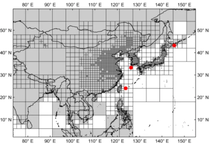
° °
Fig. 2.Map showing a zoom-in over East Asia of the variable-resolution grid (highest variable-resolution: 0.5◦×0.5◦) used for the inver-sion. The red dots denote the measurement stations. Gray boxes are considered in the inversion process and white boxes are not used.
in detail by Stohl et al. (2009), which also includes an op-timization of the baseline by the inversion scheme. Model– data mismatch uncertainties are determined as the root mean square error (RMSE) between a priori model output and ob-servation, averaged for each station, which was described in detail by Stohl et al. (2009). A variable-resolution emission grid, with grid sizes ranging from 18◦×18◦to 0.5◦×0.5◦, was used for the inversion. A zoom-in over the East Asian part of the global variable-resolution grid used for the inver-sion is shown in Fig. 2.
2.4 A priori information
In this study, we use the average value of two previous esti-mates of global SF6emissions for the years 2006–2008: (1)
that of Rigby et al. (2010) of 6500, 7140 and 7420 Mg yr−1 for 2006, 2007 and 2008, respectively, and (2) that of Levin et al. (2010) of 6290, 6790 and 7160 Mg yr−1for the same years. These estimates were linearly extrapolated to give emissions up to 2012 using the emission trend for the years 2004–2008.
We collected all available information on emissions from individual countries. The latest available UNFCCC data for more than 40 countries are for 2010 (UNFCCC, 2012a), and we assumed that emissions in 2011 and 2012 for each coun-try were equal to an average of the corresponding emis-sions from 2008–2010. In East Asia, Japan is the only Annex-I country and its reported emissions decreased from 205 Mg yr−1 in 2006 to 78 Mg yr−1 in 2010 (UNFCCC, 2012a; GIO, 2012). For South Korea, the second national communication reports emissions of 669, 707, 728 and 778 Mg yr−1 from 2006 to 2009, respectively (Republic of Ko-rea, 2012). In South KoKo-rea, Clean Development Mechanism (CDM) projects were launched in 2010 with a reduction tar-get of 86 Mg yr−1, and an additional reduction capacity of
64 Mg yr−1in 2011 (UNFCCC, 2012b), so we adopted a pri-ori emissions of 692, 628 and 628 Mg yr−1 from 2010 to 2012, respectively. For China, a priori information was de-rived from a comprehensive inventory for mainland China for 1990–2010 with a projection to 2020, which was recently made by compiling consumption and emission factor data for four industrial sources (Fang et al., 2013). For Taiwan, we adopted the values reported by the second national commu-nication submitted to the UNFCCC (Taiwan, 2011), which were 125, 125 and 129 Mg yr−1 for 2006, 2007 and 2008, respectively. They were extrapolated to 2012 by averaging the values for 2006–2008. All the national and global a pri-ori emissions used in our study are listed in Table S1 in the Supplement. The remaining emissions in all other countries (including North Korea, for which little information is avail-able) were disaggregated according to the Population Den-sity Grid Future Estimates v3 for 2010 (CIESIN, 2005). This data set was also used for gridding all national emissions.
2.5 Quantification of national emissions
We defined a “reference” inversion that uses the best avail-able a priori information (described in Sect. 2.4) and data from all stations. We performed 12 inversions with various changes made to this reference setup and report the national annual emissions as the ensemble average result. The uncer-tainty of the national emissions is estimated based on vari-ous sensitivity tests described in Sect. 3. Regarding the inver-sion ensemble, we removed the additional a priori informa-tion on China, South Korea and Taiwan, and instead assign these countries’ emissions in proportion to their fraction of the global population from non-Annex-I countries (the “no East Asia information” inversion). We also replaced our ref-erence a priori emission data set with the EDGAR (Emis-sion Database for Global Atmospheric Research) inventory (the “EDGAR” inversion). Finally, we repeated the refer-ence, no East Asia information and EDGAR inversions with the a priori emissions and their uncertainties set to 50, 100, 150, and 200 % of the value in the reference inversion. In this study, emissions from mainland China, Hong Kong and Macao were summed up and included together as emissions from “China”.
3 Results of the sensitivity tests
3.1 A priori information
We evaluated the influence of different a priori emission data sets on the inversion: (1) the reference data set, UN-FCCC and East Asian country emissions were disaggregated using the Center for International Earth Science Information Network (CIESIN, 2005) population map (UNFCCC/East Asia/CIESIN, from here on “UC_adjust”); (2) the same as UC_adjust but without East Asian country-specific in-formation (UNFCCC/CIESIN, from here on “UC”); and (3) the gridded SF6 inventory from EDGAR v4.2 (termed
“EDGAR”). Note that the emissions allocation in EDGAR is quite different from the CIESIN (2005) global popula-tion map, because EDGAR uses the urban settlements of CIESIN (2005) for an urban population map that was used as a proxy for spatial emission distribution (Janssens-Maenhout et al., 2013).
To evaluate the different a priori emission data sets, we compare the FLEXPART simulated mixing ratios using each prior with the station measurements. The mean bias between the a priori mixing ratios and observations (Ba)is the
small-est for our reference data set, UC_adjust (Supplement Ta-ble S2). For example at Gosan, the bias is only 0.165 ppt, whereas corresponding biases with EDGAR and UC emis-sions are several times higher. The a priori RMSEs (Ea)and
the squared Pearson correlation coefficients between the ob-servations and the a priori model results (ra2)values are
low-est and highlow-est, respectively, for UC_adjust at Gosan and Cape Ochi-ishi. However, at Hateruma, the EDGAR simula-tion performs better. This is because for air masses crossing Taiwan, simulation results are best using the higher EDGAR emissions for Taiwan (Supplement Table S3).
The a posteriori emissions and their distribution differ among UC_adjust, UC, and EDGAR inversions (Supplement Fig. S1). The total a posteriori emissions for China are high-est in the EDGAR inversion (2668 Mg yr−1), while values for the UC_adjust and UC inversions are lower (2312 Mg yr−1 and 2258 Mg yr−1, respectively). The reason for this is the urban clustering of emissions in the EDGAR data set, due to the constant relative emission uncertainty scaling, which leads to very high emission uncertainties in a few grid boxes. This allows the inversion (which increased Chinese emis-sions in all cases) to increase the emisemis-sions more compared with the more homogeneously distributed uncertainties in the other data sets (UC_adjust and UC). This is an effect of the clustering of high values of the emissions and their uncer-tainties in a relatively small number of grid cells in EDGAR. While our statistical comparison of the a priori and a pos-teriori model results and measurement data at Gosan and Cape Ochi-ishi was best for the UC_adjust case, the EDGAR case was slightly better at Hateruma (Table S2 in the Supple-ment). Therefore, averages of the a posteriori emissions from all three cases were used for reporting national emissions in Sect. 4.
3.2 Emission uncertainty
We tested the uncertainty scaling in a similar way to Keller et al. (2011) by employingσxj=p·maxh0.5xj,1.0xsurfiand
varying the uncertainty scale factorp, withxj being the a priori emission flux in inversion boxj, andxsurfthe average
land surface emission flux. The results in terms of a compar-ison of modeled and measured mixing ratios are shown in Supplement Fig. S2. There is a nearly monotonic decrease in the RMSE and an increase in the correlation coefficient with increasing values ofp, i.e., when the constraint to the a priori emissions is relaxed. However, there is hardly any change in the model skill forpvalues larger than 5. At the same time, whenp values increase, so does the danger of overfitting the observations as the a priori constraint is weak-ened. The a posteriori emission maps show increasing lev-els of noise for these largepvalues. For instance, artificially high emissions for SF6were produced forp> 5 in
southwest-ern China, which cannot be explained by known sources. The exact choice of the scale factor remains subjective, but from these tests a value of 1 appears most appropriate and was therefore used for our inversions.
3.3 Inversion resolution and geometry
A source of a posteriori emission errors in the country to-tals is the attribution of emissions in border regions to one of the neighboring countries. This is especially problematic for smaller countries like North and South Korea. A compar-ison of the a posteriori emissions when using 0.5◦×0.5◦and 1◦×1◦as the maximum grid resolution is shown in Supple-ment Fig. S3. The total national a posteriori emissions do not change much for large countries; for example, a posteriori emissions for China and Japan differ by only 0 and 1 % for these two inversions, respectively. However, for North Korea and South Korea, emissions are 28 % higher and−7 % lower with the coarser resolution, respectively. The emissions are about 10 times higher for South Korea than for North Korea, and large emissions occur near the political border. With the coarser resolution, more of these emissions are erroneously attributed to North Korea. Simulated mixing ratios, however, are very similar for the coarse- and fine-resolution inversions. For instance, the squared Pearson correlation coefficients be-tween the observations and the a posteriori model results (rb2) values for Gosan, Hateruma and Cape Ochi-ishi change by only 0.001–0.009 when degrading the resolution to 1◦×1◦.
for Gosan, Hateruma and Cape Ochi-ishi, respectively. The emission estimates for larger countries are also stable, while relative differences are larger for smaller countries. Tests showed that the a posteriori emission distribution patterns re-mained relatively stable when more than about 1500 boxes were used. Thus, we chose about 2500 boxes for our inver-sions.
3.4 Station network
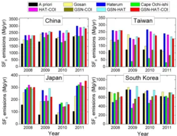
Inversion results may be quite sensitive to adding or remov-ing a station. Since no time series is completely continuous, data gaps are equivalent to effectively “adding” or “remov-ing” a station for the duration of the gap. Therefore, we tested the influence of adding/removing stations on the a posteriori SF6 emissions in East Asia. Figure 3 shows the national a
priori and a posteriori emissions in each year from the ref-erence inversion but using either one, two or three stations in East Asia (Mace Head and Trinidad Head were used in all these tests). The difference between the a priori and a posteriori emissions is generally smaller when only one sta-tion is used compared to when more than one stasta-tion is used in the inversion. The impact of the different stations for the national emission estimates is quite different. A posteriori emissions for China and Taiwan when using only Hateruma data, for instance, are quite close to the corresponding three-station result, while using only Gosan or Cape Ochi-ishi data yields a posteriori emissions much closer to the a priori val-ues. This is probably due to the fact that footprint emission sensitivity values in Taiwan and southern China are highest for Hateruma (see Fig. 1).
3.5 Meteorological input data
To evaluate the influence of meteorological input data res-olution, 0.25◦×0.25◦ ECMWF data for East Asia (100 to 150◦E, 10 to 50◦N) were nested (termed “Nest_ECMWF”) into the global 1.0◦×1.0◦ECMWF data used without nest-ing for our reference inversion (termed “ECMWF”). The Nest_ECMWF simulations generally improve the model per-formance compared to the observations in terms of bias, RMSE and correlation obtained for simulated versus ob-served mixing ratios at the three stations (Supplement Ta-ble S4). This holds both for a priori and a posteriori re-sults. For example, in the ECMWF case (Nest_ECMWF case) the rb2 values are 0.45 (0.49), 0.58 (0.65) and 0.76 (0.77) for Gosan, Hateruma and Cape Ochi-ishi, respec-tively. However, a posteriori national emission totals are similar (Supplement Table S5) – e.g., 2312 (ECMWF) and 2355 (Nest_ECMWF) Mg yr−1 for China – and there is a difference of only 3 % for total emissions from East Asia. Thus, while dispersion model results are slightly better with nested data (e.g.,ra2=0.26 for ECMWF case and 0.32 for Nest_ECMWF case), the national emission totals obtained from the inversion are relatively stable. Therefore, only
–
Fig. 3.A priori and a posteriori national SF6 emissions in East Asia for the years 2008–2011. A posteriori results are from the reference inversion but using measurement data from only one, two or all three East Asian measurement stations (GSN=Gosan, HAT=Hateruma and COI=Cape Ochi-ishi).
global meteorological data were used for our yearly inver-sions.
Results for inversions using CFSR and FNL data are also shown in Supplement Tables S4 and S5. There is no one data set that is consistently better than the others. The per-formance statistics show that for Gosan and Cape Ochi-ishi, the ECMWF data yield best results, while for Hateruma, the FNL data seem to work better. However, even for a given site the best-performing data set changes with time. For instance, Fig. 4 shows the mixing ratio time series for Hateruma in 2008 and an example of emission sensitivities for highlighted cases is shown in Supplement Fig. S5. Overall, ECMWF simulations performed slightly better than the other data sets, but only the Nest_ECMWF simulations give the best results for almost all stations and for almost all statistical param-eters. It is difficult to say what exactly causes the different model performances for the non-nested cases. One reason may be the higher vertical resolution of the ECMWF data (92 levels compared to 37 and 26 levels for CSFR and FNL). Temporal resolution may be another factor. While ECMWF and CFSR data were used with 3-hourly resolution, the FNL data are 6-hourly. Certainly there are many other differences between the different meteorological data sets such as the underlying physical model and data assimilation scheme.
3.6 Seasonal variability
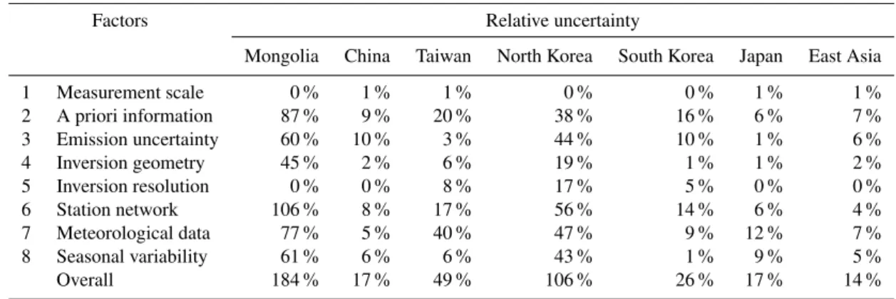
Table 2.Relative uncertainties of a posteriori SF6emissions in East Asia as obtained from the different sensitivity tests, as well as total uncertainty assuming that the individual errors are independent.
Factors Relative uncertainty
Mongolia China Taiwan North Korea South Korea Japan East Asia
1 Measurement scale 0 % 1 % 1 % 0 % 0 % 1 % 1 %
2 A priori information 87 % 9 % 20 % 38 % 16 % 6 % 7 %
3 Emission uncertainty 60 % 10 % 3 % 44 % 10 % 1 % 6 %
4 Inversion geometry 45 % 2 % 6 % 19 % 1 % 1 % 2 %
5 Inversion resolution 0 % 0 % 8 % 17 % 5 % 0 % 0 %
6 Station network 106 % 8 % 17 % 56 % 14 % 6 % 4 %
7 Meteorological data 77 % 5 % 40 % 47 % 9 % 12 % 7 %
8 Seasonal variability 61 % 6 % 6 % 43 % 1 % 9 % 5 %
Overall 184 % 17 % 49 % 106 % 26 % 17 % 14 %
Fig. 4.Observed and simulated SF6 mixing ratio time series at Hateruma station when using ECMWF, CFSR and FNL meteoro-logical data for 2008. Pollution episodes labeled(a), (b) and(c) were best simulated by using the CFSR, FNL and ECMWF data set, respectively.
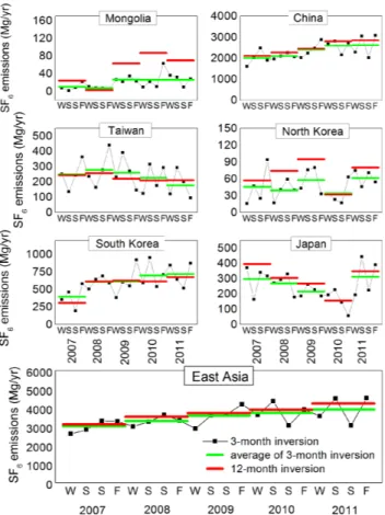
(March, April, May), summer (June, July, August) and au-tumn (September, October, November). For these inversions, and for the whole-year inversion used for comparison, the number of emission boxes was reduced to about 1500 be-cause of the reduced number of measurements. Five-year seasonal variations of SF6 a posteriori emissions for each
East Asian country show that there is no regular seasonal-ity of the retrieved SF6emissions (Fig. 5). For example, for
China, in 2007 the inferred emissions are highest in sum-mer, while in 2011 the emissions in summer are the lowest. This irregular emission variability is the same in the other
five countries/regions. This is not very surprising, because no seasonality is expected for the major SF6source categories.
Figure 5 shows that the average of the a posteriori emis-sions from four seasonal inveremis-sions is close to the a posteriori emissions from the whole-year inversion for the same year. For the years 2007–2011, the relative differences between the mean of the seasonal inversions and the reference inversion are−7±4 % for China, 2±17 % for Taiwan,−18±35 % for North Korea, 8±13 % for South Korea, −6±8 % for Japan and−6±2 % for East Asia.
3.7 Overview of the sensitivity tests
Table 2 presents an overview of the uncertainties of national emissions obtained from the different sensitivity tests for the year 2008. It is not possible to derive an exact value for the posterior uncertainty as this requires exact knowledge of the transport errors, prior errors and observation errors and their correlations. However, our sensitivity tests provide an ap-proximation for the uncertainty from these components. For testi, we report the relative uncertainty Ui as the standard deviation of the a posteriori emissions divided by the mean of the ensemble inversions in testi. Assuming that the uncer-tainties fromN sensitivity tests performed are independent from each other (in reality they are not completely indepen-dent, but their correlation is not known), we report the total relative uncertainty asU=
q
PN
Fig. 5.Seasonal variations of SF6a posteriori emissions for each East Asian country for the 2007–2011 period. Black dots denote a posteriori emissions from seasonal inversions; green lines denote an average of a posteriori emissions from four seasonal inversions in each year; red lines denote a posteriori emissions from the refer-ence inversion using the whole-year observation data. W, S, S and F on thexaxis represent winter (December, January, and February), spring (March, April, and May), summer (June, July and August) and fall (September, October and November) in each year, respec-tively.
errors, such as model biases, e.g., under- or overestimation of boundary layer heights, which may be important especially for countries like China where the reported stochastic errors are small.
4 National total emissions and emission distribution 4.1 National emissions
National emissions as obtained from the inversion are re-ported in Table 3, with uncertainties (indicated by±values) derived from the overall relative uncertainties as obtained in the sensitivity tests. These uncertainty estimates are larger than the uncertainties obtained from error propagation in a single reference inversion. Measurement statistics and inver-sion performance for the period 2006–2012 are shown in
Supplement Table S6, and time series of the measured and simulated SF6mixing ratios for 2011 are shown as an
exam-ple in Supexam-plement Fig. S6.
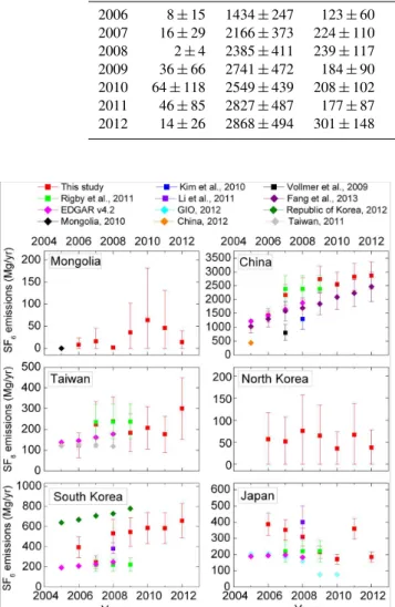
Comparisons of our estimates with other published es-timates are shown in Fig. 6. For China, our best esti-mate for 2008, 2385±411 Mg yr−1, is larger than the es-timate of 1300 (930–1700) Mg yr−1 reported by Kim et al. (2010) and agrees within uncertainty with the value of 2383 (1867–2865) Mg yr−1 for 2007–2009 reported by Rigby et al. (2011). Our estimate for 2007 is also much larger than the estimate of Vollmer et al. (2009) for the same year, although the emissions of other halocarbons esti-mated by Vollmer et al. (2009) are higher than those reported in other studies (Stohl et al., 2010; Li et al., 2011). Com-pared with the bottom-up estimates of Fang et al. (2013) and EDGAR (2011), our estimates are slightly higher (especially for years 2007–2009) but with consistent emission trends.
For Taiwan, the a posteriori emissions are consistent with the estimated emissions by Rigby et al. (2011), but are about two times higher than the bottom-up estimates in the sec-ond national communication of Taiwan for the years 2007 and 2008 (Taiwan, 2011). For South Korea, the inversion re-sults are always lower than bottom-up estimates in the South Korea national communication (Republic of Korea, 2012). However, our estimates for the years 2008 and 2009 are about twice as high as estimates by Li et al. (2011) and Rigby et al. (2011). This is not due to a too-high a priori adopted in our inversion because a posteriori values of the same magni-tude were still obtained even with the a priori value cut by 50 %. For Japan, our estimates agree within the uncertainty range with the ratio-method estimates of Li et al. (2011) and the inversion estimates of Rigby et al. (2011). The reported emissions to UNFCCC and EDGAR estimates are lower than our estimates for Japan.
The emission trends were very different in East Asian countries during the 2006–2012 period. For Japan, one of the Annex-I countries under UNFCCC, inversion results show that its emissions are decreasing except for the year 2011. From 2008 to 2009, there is a relatively large decrease in emissions from 309±54 Mg yr−1 to 215±38 Mg yr−1, which is partly due to a reported reduction of 43 Mg yr−1 caused by the equipment of SF6 manufacturing facilities
with recovery/destruction units and reported additional re-ductions of 17 Mg yr−1in the magnesium foundry sector and 11 Mg yr−1in the semiconductor manufacture sector in 2009 (GIO, 2012). The emission anomaly in 2011 is very likely caused by leakage to the atmosphere of SF6 enclosed in
certain high-voltage electrical insulation equipment due to the damage caused by the Great East Japan Earthquake on 11 March 2011. Seasonal inversions show that the increase is largely due to extraordinarily high emissions in spring, con-sistent with a source related to the earthquake. Indeed, loss of SF6due to earthquake damage was reported by some
Table 3.SF6emissions (Mg yr−1) per country/region for the period 2006–2012. Results are shown for the mean a posteriori emissions from the inversion ensemble, and the corresponding uncertainties estimated based on the overall relative uncertainties in Table 2.
Mongolia China Taiwan North Korea South Korea Japan East Asia
2006 8±15 1434±247 123±60 57±60 395±104 387±68 2404±325 2007 16±29 2166±373 224±110 52±55 246±65 352±62 3056±413 2008 2±4 2385±411 239±117 76±81 532±140 309±54 3542±479 2009 36±66 2741±472 184±90 65±69 546±143 215±38 3787±512 2010 64±118 2549±439 208±102 36±38 586±154 172±30 3616±489 2011 46±85 2827±487 177±87 67±71 584±153 360±63 4061±549 2012 14±26 2868±494 301±148 38±40 657±172 185±32 4063±549
Fig. 6.Comparison of our a posteriori national emission estimates with other published estimates, as specified in the legend at the top. Square symbols denote top-down estimates and diamond symbols denote bottom-up estimates.
For China, the a posteriori emissions almost doubled dur-ing 2006–2012, reflectdur-ing a fast increase of SF6
consump-tion and emissions in China. Usage of SF6 in the electrical
equipment sector was estimated to have increased from about 820 Mg yr−1in 2001 to 4990 Mg yr−1in 2010, with a bigger leap in the first five years. Usage of SF6in the semiconductor
manufacturing sector and the magnesium production sector also increased by about 4 times and the total of these two sectors accounts for one-eighth of that in the electrical equip-ment sector (Fang et al., 2013). Considering the increase of usage during the period 2001–2010 and the delay between its employment and its emissions in the electrical equipment sector, an emission increase during 2006–2012 is expected.
For South Korea, emissions increase from 2006 to 2012, with an exception in 2007. CDM projects with 86 Mg yr−1 reduction capacity and additional 64 Mg yr−1 reduction ca-pacity were launched in 2010 and in 2011, respectively. Without these CDM reductions, the SF6emissions in South
Korea would most likely have increased more strongly. For Taiwan, communications to the UNFCCC report increasing emissions from 2000 to 2008 (Taiwan, 2011), and we find a decrease from about the year 2008, suggesting emissions from Taiwan peaked around the year 2008. However, emis-sions for 2012 are estimated to be much higher than those in previous years. Emissions from North Korea and Mongolia are very small and there are no significant trends. For North Korea, it is possible that some of the emissions are actually due to South Korean sources close to the border, which could not be correctly attributed by the inversion.
The SF6emissions from East Asia as a whole (Fig. 7,
up-per left) grew gradually from 2404±325 Mg yr−1in 2006 to 3787±512 Mg yr−1in 2009 and stabilized afterwards. The global SF6emissions for the period 2006–2008 have likely
increased almost linearly (see Supplement Table S1). The contribution from emissions in East Asia to the global total increased from 38±5 % in 2006 to 49±7 % in 2009. Based on extrapolated global emissions (see Sect. 2.4), the contri-butions of East Asia to the global totals stabilized between 49±7 and 45±6 % for the period 2009–2012.
The major contribution to East Asian emissions is from China (Fig. 7, upper right), accounting for 60–72 % depend-ing on the year, followed by South Korea (8–16 %), Japan (5–16 %) and Taiwan (4–7 %), while emissions from North Korea and Mongolia together contribute less than 3 %. Taken on a per capita basis, SF6emissions in China and Japan are
close to the global average (Fig. 7, bottom). On the other hand, per capita emissions from South Korea and Taiwan are more than 5 times the global per capita emissions.
4.2 Spatial emission distribution and Chinese provincial emissions
Fig. 7.Global perspective of SF6emissions of East Asian countries. The upper left panel shows absolute (black symbols and leftyaxis) and relative contributions (orange symbols and rightyaxis) of emis-sions in East Asia to the global totals. The upper right panel shows relative contributions of emissions from each country within East Asia. The lower panel shows per capita emissions for each country, with the yellow line indicating the global average.
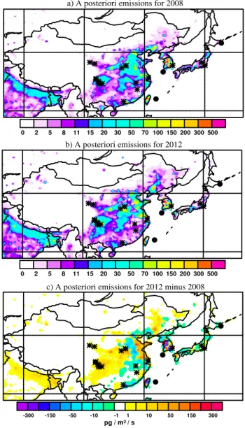
are in South Korea, where the liquid-crystal display (LCD) sector and electrical equipment sector are two important emission sources. Several abatement CDM projects were launched in the LCD sector in 2010 and 2011, so it is seen that emissions from some of the boxes containing LCD fac-tories have decreased afterwards. However, we have to con-sider the compensation by emission increases from other sources located in the same boxes. For Taiwan, the emis-sions are higher in the west than in the east, as the popu-lation is denser and there is more industry along the western coastline. For Japan, high emission fluxes occur in the re-gions of Tokyo, Osaka and Nagoya. For China, high emis-sions are concentrated in Liaoning and Jilin (northeastern China), Beijing, Hebei, Shanxi and Henan (northern China), Shandong, Jiangsu, Shanghai and Zhejiang (eastern China) and Sichuan (southwestern China) provinces. The locations of factories known to have produced SF6 around the year
2008 (Xiao, 2010; Cheng, 2010) are also marked in Fig. 8. Almost all Chinese factories are shown on the map, but this was not used as a priori information in the inversion. While loss during SF6 production is only one source of SF6,
esti-mated as 7.5 % of the inventory total emission in China (Fang et al., 2013), most of the factory locations are associated with high a posteriori emissions by the inversion. However, in China, emissions from electrical equipment dominate, ac-counting for more than 70 % of national totals based on the estimates by Fang et al. (2013). Hundreds of thousands of individual devices containing SF6have been reported in the
yearbook (CEPP, 2010), leading to widespread distribution
a) A posteriori emissions for 2008
b) A posteriori emissions for 2012
c) A posteriori emissions for 2012 minus 2008
Fig. 8.Maps of the a posteriori SF6emissions for 2008 (top panel) and 2012 (middle panel), and difference between a posteriori emis-sions for 2012 and those for 2008 (bottom panel). Black dots denote the location of measurement stations. Asterisks mark the locations of factories in East Asia known to have produced SF6around the year 2008.
of SF6 emission sources. During 2008–2012, emission
5 Conclusion
We have performed a large number of sensitivity tests to quantify the uncertainties associated with our inversion setup. We found that the most important sources of uncer-tainty associated with the inversions are related to the a pri-ori emissions used and their assumed uncertainty, the station network as well as the meteorological input data. Much lower uncertainties are due to seasonal emission variability, inver-sion geometry, inverinver-sion resolution and measurement cali-bration scale. The overall relative uncertainties of the na-tional a posteriori emissions are 184, 17, 49, 106, 26 and 17 % for Mongolia, China, Taiwan, North Korea, South Ko-rea and Japan, respectively.
Based on the sensitivity tests, we employed the optimal parameters in our inversion setup and performed yearly in-versions for the period 2006–2012. Results show that the SF6 emissions from East Asia as a whole grew gradually
from 2404±325 Mg yr−1 in 2006 to 3787±512 Mg yr−1 in 2009 and stabilized afterwards. Contributions from East Asia to global emissions are estimated to be between 38±5 and 49±7 % in different years. The major contributor to the East Asian totals is China (60–72 % depending on the year), followed by South Korea (8–16 %), Japan (5–16 %) and Taiwan (4–7 %), while emissions from North Korea and Mongolia together were less than 3 % of the total. Chi-nese emissions increased from 1434±247 Mg yr−1in 2006 to 2741±472 Mg yr−1 in 2009 and did not change much afterwards. Emissions from South Korea increased from 395±104 Mg yr−1 in 2006 to 657±172 Mg yr−1 in 2012,
while emissions from Taiwan and Japan have decreased over-all. The per capita SF6 emissions in South Korea and
Tai-wan are more than 5 times the global per capita emissions, while per capita emissions for China, North Korea and Japan are close to the global average. Emission spatial distributions changed differently in different parts of East Asia. For exam-ple, while the total Chinese emissions increased gradually, there were large regional differences.
Supplementary material related to this article is available online at http://www.atmos-chem-phys.net/14/ 4779/2014/acp-14-4779-2014-supplement.pdf.
Acknowledgements. We acknowledge use of ECMWF, CFSR
and FNL meteorological data. Atmospheric observations at Hateruma and Cape Ochi-ishi stations were supported by the Global Environment Fund (Ministry of the Environment of Japan). Measurements at Gosan station were supported by the National Research Foundation of Korea (NRF, no. 2010-0029119). We thank the Atmospheric Chemistry Research Group, University of Bristol (UB), United Kingdom, and Scripps Institution of Oceanography (SIO), University of California, United States, for running the Mace Head and Trinidad Head AGAGE stations, respectively,
and SIO for providing the calibrations for these two stations and Gosan. We acknowledge J. Mühle (SIO) and Christina Harth (SIO) for their great contribution to the intercalibration between NIES-2008 and SIO-2005. We also acknowledge use of EDGAR and UNFCCC emission data, and CIESIN gridded population data. The financial support provided by the China Scholarship Council (no. 201206010235) during a one-year visit of X. Fang to the Norwegian Institute for Air Research is gratefully acknowledged. The Norwegian Research Council also provided partial support through the SOGG-EA project (no. 193774).
Edited by: G. Stiller
References
CEPP: China Electric Power Yearbook, China Electric Power Press (CEPP), Beijing, China, 2010 (in Chinese).
Cheng, H.: Competitive Strength and Market Analysis of Elec-tronic Chemicals and Special Gas Containing Fluorine, Chemical Production and Technology, 17, 1–7, doi:10.3969/j.issn.1006-6829.2010.06.001, 2010 (in Chinese with English abstract). China: Second National Communication on Climate Change of The
People’s Republic of China, National Development and Reform Commission of China, Beijing, China, 2012.
CIESIN: Gridded Population of the World: Future Estimates (GPWFE), Center for International Earth Science Informa-tion Network (CIESIN), http://sedac.ciesin.columbia.edu/data/ collection/gpw-v3 (last access: 7 November 2012), 2005. Democratic People’s Republic of Korea: DPRK’s first national
communication under the Framework Convention on Climate Change, Ministry of Land and Environment Protection, Demo-cratic People’s Republic of Korea, 2000.
EDGAR: Emission Database for Global Atmospheric Research (EDGAR), release version 4.2, European Commission, Joint Research Centre (JRC)/Netherlands Environmental Assess-ment Agency (PBL), http://edgar.jrc.ec.europa.eu (last access: 22 March 2012), 2011.
Enomoto, T., Yokouchi, Y., Izumi, K., and Inagaki, T: Development of an analytical method for atmospheric halocarbons and its ap-plication to airborne observation, J. Jpn. Soc. Atmos. Environ., 40, 1–8, 2005 (in Japanese).
Fang, X., Hu, X., Janssens-Maenhout, G., Wu, J., Han, J., Su, S., Zhang, J., and Hu, J.: Sulfur hexafluoride (SF6) emis-sion estimates for China: an inventory for 1990–2010 and a projection to 2020, Environ. Sci. Technol., 47, 3848–3855, doi:10.1021/es304348x, 2013.
Forster, P., Ramaswamy, V., Artaxo, P., Berntsen, T., Betts, R., Fa-hey, D. W., Haywood, J., Lean, J., Lowe, D. C., Myhre, G., Nganga, J., Prinn, R., Raga, G., Schulz, M., and Dorland, R. V.: Changes in Atmospheric Constituents and in Radiative Forc-ing, in: Climate Change 2007: The Physical Science Basis. Con-tribution of Working Group I to the Fourth Assessment Report of the Intergovernmental Panel on Climate Change, edited by: Solomon, S., Qin, D., Manning, M., Chen, Z., Marquis, Z., Av-ery, K. B., Tignor, M., and Miller, H. L., Cambridge University Press, Cambridge, UK, 129–234, 2007.
Environmental Studies (NIES), Ministry of the Environment, Japan, 2012.
Hall, B. D., Dutton, G. S., Mondeel, D. J., Nance, J. D., Rigby, M., Butler, J. H., Moore, F. L., Hurst, D. F., and Elkins, J. W.: Improving measurements of SF6 for the study of atmospheric transport and emissions, Atmos. Meas. Tech., 4, 2441–2451, doi:10.5194/amt-4-2441-2011, 2011.
Hitachi Cable, Ldt.: Report on the Great East Japan Earthquake: Global Warming Prevention, Hitachi Cable, Ltd., Japan, 2011. Janssens-Maenhout, G., Diego, V. P., and Marilena Muntean,
G.: Global emission inventories in the Emission Database for Global Atmospheric Research (EDGAR) – Manual (I). Gridding: EDGAR emissions distribution on global gridmaps, Publications Office of the European Union, Luxembourg, 2013.
Kim, J., Li, S., Kim, K. R., Stohl, A., Mühle, J., Kim, S. K., Park, M. K., Kang, D. J., Lee, G., Harth, C. M., Salameh, P. K., and Weiss, R. F.: Regional atmospheric emissions deter-mined from measurements at Jeju Island, Korea: Halogenated compounds from China, Geophys. Res. Lett., 37, L12801, doi:10.1029/2010GL043263, 2010.
Keller, C. A., Brunner, D., Henne, S., Vollmer, M. K., O’Doherty, S., and Reimann, S.: Evidence for under-reported western Euro-pean emissions of the potent greenhouse gas HFC-23, Geophys. Res. Lett., 38, L15808, doi:10.1029/2011gl047976, 2011. Levin, I., Naegler, T., Heinz, R., Osusko, D., Cuevas, E., Engel, A.,
Ilmberger, J., Langenfelds, R. L., Neininger, B., Rohden, C. v., Steele, L. P., Weller, R., Worthy, D. E., and Zimov, S. A.: The global SF6source inferred from long-term high precision atmo-spheric measurements and its comparison with emission invento-ries, Atmos. Chem. Phys., 10, 2655–2662, doi:10.5194/acp-10-2655-2010, 2010.
Li, S., Kim, J., Kim, K. R., Mühle, J., Kim, S. K., Park, M. K., Stohl, A., Kang, D. J., Arnold, T., Harth, C. M., Salameh, P. K., and Weiss, R. F.: Emissions of Halogenated Compounds in East Asia Determined from Measurements at Jeju Island, Korea, Environ. Sci. Technol., 45, 5668–5675, doi:10.1021/Es104124k, 2011. Miller, B. R., Weiss, R. F., Salameh, P. K., Tanhua, T., Greally, B.
R., Mühle, J., and Simmonds, P. G.: Medusa: A sample precon-centration and GC/MS detector system for in situ measurements of atmospheric trace halocarbons, hydrocarbons, and sulfur com-pounds, Anal. Chem., 80, 1536–1545, doi:10.1021/Ac702084k, 2008.
Mongolia: Mongolia second national communication under the United Nations Framework Convention on Climate Change, Ministry of Nature, Environment and Tourism, Ulaanbaatar, Mongolia, 2010.
Olivier, J. G. J., Van Aardenne, J. A., Dentener, F., Ganzeveld, L., and Peters, J. A. H. W.: Recent trends in global greenhouse gas emissions: regional trends and spatial distribution of key sources, in: Non-CO2Greenhouse Gases (NCGG-4), edited by: van Am-stel, A., Millpress, Rotterdam, the Netherlands, 325–330, 2005. Prinn, R. G., Weiss, R. F., Fraser, P. J., Simmonds, P. G.,
Cun-nold, D. M., Alyea, F. N., O’Doherty, S., Salameh, P., Miller, B. R., Huang, J., Wang, R. H. J., Hartley, D. E., Harth, C., Steele, L. P., Sturrock, G., Midgley, P. M., and McCulloch, A.: A his-tory of chemically and radiatively important gases in air de-duced from ALE/GAGE/AGAGE, J. Geophys. Res., 105, 17751– 17792, doi:10.1029/2000jd900141, 2000.
Ravishankara, A. R., Solomon, S., Turnipseed, A. A., and War-ren, R. F.: Atmospheric Lifetimes of Long-Lived Halogenated Species, Science, 259, 194–199, 1993.
Republic of Korea: Korea’s third national communication under the United Nations Framework Convention on Climate Change, Ministry of Environment, Seoul, The Republic of Korea, 2012. Rigby, M., Mühle, J., Miller, B. R., Prinn, R. G., Krummel, P.
B., Steele, L. P., Fraser, P. J., Salameh, P. K., Harth, C. M., Weiss, R. F., Greally, B. R., O’Doherty, S., Simmonds, P. G., Vollmer, M. K., Reimann, S., Kim, J., Kim, K.-R., Wang, H. J., Olivier, J. G. J., Dlugokencky, E. J., Dutton, G. S., Hall, B. D., and Elkins, J. W.: History of atmospheric SF6from 1973 to 2008, Atmos. Chem. Phys., 10, 10305–10320, doi:10.5194/acp-10-10305-2010, 2010.
Rigby, M., Manning, A. J., and Prinn, R. G.: Inversion of long-lived trace gas emissions using combined Eulerian and Lagrangian chemical transport models, Atmos. Chem. Phys., 11, 9887–9898, doi:10.5194/acp-11-9887-2011, 2011.
Stohl, A., Hittenberger, M., and Wotawa, G.: Validation of the La-grangian particle dispersion model FLEXPART against large-scale tracer experiment data, Atmos. Environ., 32, 4245–4264, doi:10.1016/s1352-2310(98)00184-8, 1998.
Stohl, A., Forster, C., Frank, A., Seibert, P., and Wotawa, G.: Technical note: The Lagrangian particle dispersion model FLEXPART version 6.2, Atmos. Chem. Phys., 5, 2461–2474, doi:10.5194/acp-5-2461-2005, 2005.
Stohl, A., Seibert, P., Arduini, J., Eckhardt, S., Fraser, P., Greally, B. R., Lunder, C., Maione, M., Mühle, J., O’Doherty, S., Prinn, R. G., Reimann, S., Saito, T., Schmidbauer, N., Simmonds, P. G., Vollmer, M. K., Weiss, R. F., and Yokouchi, Y.: An analytical inversion method for determining regional and global emissions of greenhouse gases: Sensitivity studies and application to halo-carbons, Atmos. Chem. Phys., 9, 1597–1620, doi:10.5194/acp-9-1597-2009, 2009.
Stohl, A., Kim, J., Li, S., O’Doherty, S., Mühle, J., Salameh, P. K., Saito, T., Vollmer, M. K., Wan, D., Weiss, R. F., Yao, B., Yokouchi, Y., and Zhou, L. X.: Hydrochlorofluoro-carbon and hydrofluoroHydrochlorofluoro-carbon emissions in East Asia deter-mined by inverse modeling, Atmos. Chem. Phys., 10, 3545– 3560, doi:10.5194/acp-10-3545-2010, 2010.
Taiwan: Second National Communication of the Republic of China (Taiwan) under the United Nations Framework Convention on Climate Change Executive Summary, 2011.
Tohjima, Y., Machida, T., Utiyama, M., Katsumoto, M., Fujinuma, Y., and Maksyutov, S.: Analysis and presentation of in situ atmospheric methane measurements from Cape Ochi-ishi and Hateruma Island, J. Geophys. Res., 107, ACH 8-1–ACH 8-11, doi:10.1029/2001jd001003, 2002.
UN: Kyoto Protocol to the United Nations Framework Convention on Climate Change, United Nations, 1998.
UNFCCC: Flexible GHG data queries, United Nations Framework Convention on Climate Change (UNFCCC), http://unfccc.int/di/ FlexibleQueries.do (last access: 21 December 2012), 2012a. UNFCCC: United Nations Framework Convention on Climate
Change: Clean Development Mechanism (CDM), http://cdm. unfccc.int/Projects/projsearch.html (last access: 20 December 2012), 2012b.
M., Zhang, F., Huang, J., and Simmonds, P. G.: Emissions of ozone-depleting halocarbons from China, Geophys. Res. Lett., 36, L15823, doi:10.1029/2009gl038659, 2009.
Xiao, M. L.: Development analysis of domestic sulfur hexafluoride industry, Chemical Propellants & Polymeric Materials, 8, 65–67, 2010 (in Chinese with English abstract).