OASIS4 – a coupling software for next generation earth system modelling

(1)

GMDD

2, 797–843, 2009

The OASIS4 software for coupled climate

modelling

R. Redler et al.

Title Page

Abstract Introduction

Conclusions References

Tables Figures

◭ ◮

Back Close

Full Screen / Esc

Printer-friendly Version

Interactive Discussion

Geosci. Model Dev. Discuss., 2, 797–843, 2009 www.geosci-model-dev-discuss.net/2/797/2009/ © Author(s) 2009. This work is distributed under the Creative Commons Attribution 3.0 License.

Geoscientific Model Development Discussions

Geoscientific Model Development Discussionsis the access reviewed discussion forum ofGeoscientific Model Development

OASIS4 – a coupling software for next

generation earth system modelling

R. Redler1, S. Valcke2, and H. Ritzdorf1

1

NEC Research Laboratories, NEC Europe Ltd., Sankt Augustin, Germany

2

CERFACS, Toulouse, France

Received: 19 June 2009 – Accepted: 22 June 2009 – Published: 7 July 2009 Correspondence to: R. Redler ([email protected])

(2)

GMDD

2, 797–843, 2009

modelling

R. Redler et al.

Title Page

Tables Figures

◭ ◮

Back Close

Full Screen / Esc

Abstract

In this article we present a new version of the Ocean Atmosphere Sea Ice Soil coupling software (OASIS4). With this new fully parallel OASIS4 coupler we target the needs of Earth system modelling in its full complexity. The primary focus of this article is to describe the design of the OASIS4 software and how the coupling software drives the

5

whole coupled model system ensuring the synchronization of the different component models. The application programmer interface (API) manages the coupling exchanges between arbitrary climate component models, as well as the input and output from and to files of each individual component. The OASIS4 Transformer instance performs the parallel interpolation and transfer of the coupling data between source and target

10

model components. As a new core technology for the software, the fully parallel search algorithm of OASIS4 is described in detail. First benchmark results are discussed with simple test configurations to demonstrate the efficiency and scalability of the software when applied to Earth system model components. Typically the compute time needed in order to perform the search is in the order of a few seconds and is only weakly

15

dependant on the grid size.

1 Introduction

Global coupled models (GCMs) have been used for climate simulations since the late 1960s starting with the pioneering work by Manabe and Bryan (1969). With advances in computing power, coupled models have been in use for century-long simulations

20

since the late 1980s. Since that time, we observe a rapid and continuous increase of activity in global coupled modelling as additional computer resources have become available. Climate models can be considered as multi-disciplinary or multi-physics soft-ware tools to simulate the interactions of the atmosphere, oceans, land surface, sea ice and other components of the climate system. They are used for a variety of

pur-25

(3)

GMDD

2, 797–843, 2009

modelling

R. Redler et al.

Title Page

Tables Figures

◭ ◮

Back Close

Full Screen / Esc

of future climate. These models can range from relatively simple to quite complex, that is from zero-dimensional models and Earth-system Models of Intermediate Complexity (EMIC) to complex 3-dimensional Global Climate Models (GCM) and Regional Climate Models (RCM).

A GCM aims to describe geophysical flow by integrating a variety of fluid-dynamical,

5

chemical, or even biological equations that are either derived directly from physical laws (e.g. Newton’s law) or constructed by more empirical means. Classically, the two main constituents of a GCM are atmospheric and ocean circulation models. When coupled together (along with other components such as a sea ice model and a land model) an ocean-atmosphere coupled general circulation model forms the basis for a

10

full climate model. A very recent trend in GCMs is to extend these traditional coupled climate models to become full Earth system models (ESM), by including further model components e.g. for atmospheric chemistry, marine biology or a carbon cycle model (matter cycle in a more general sense) to more correctly simulate the interaction be-tween the different sub-components. Typically, these different model components are

15

developed independently by different research groups.

Numerical modelling in its full complexity is still in its infancy, primarily due to the immense complexity of the task and insufficient empirical knowledge of many aspects of climate related processes. This is not only the case for the oceans where in par-ticular the knowledge of the subsurface circulation is rather poor, but also for the

hy-20

drological cycle where precipitation, evaporation and the three-dimensional distribution of water vapour and clouds are insufficiently known. Despite these uncertainties the development of global climate models is one of the main unifying components in the World Climate Research Programme (WCRP) of the World Meteorological Organisa-tion (WMO). The output of these models is considered as fundamental deliverables

25

(4)

(CLI-GMDD

2, 797–843, 2009

modelling

R. Redler et al.

Title Page

Tables Figures

◭ ◮

Back Close

Full Screen / Esc

VAR) or the Coupled Model Intercomparison Project (CMIP) as one of the CLIVAR ini-tiatives, not to forget efforts on a more regional scale like EuroCLIVAR, the Baltic Sea Experiment (BALTEX) or the North American Regional Climate Change Assessment Program (NARCCAP), just to mention a few. Most important, global climate models form one of the backbones of the Assessment Reports (AR) published by the

Intergov-5

ernmental Panel of Climate Change (IPCC).

In addition to the model components used in an ESM, each community representing one of the physical components still feels a strong need for having separate stand-alone special-purpose versions of the individual components of the coupled climate models to investigate processes in the different subsystems and to test new physical

10

parameterisations in controlled scenario runs. The existence of di_fferent research ob-jectives and the need to estimate model uncertainty from model intercomparison (like for the IPCC AR) support the idea of a multi-component approach and the need for the interoperability of the di_fferent components. A multi-component approach helps to avoid complex technical problems arising from an all-in-one code integrating

indepen-15

dently developed components. Furthermore independent codes are of great advan-tage for the flexibility of the system (D ¨oscher et al., 2002). It is therefore only natural to consider a coupling of any two or more physical component models through some independent coupling software ensuring the lowest possible degree of interference in the component codes themselves.

20

With OASIS4, we continue the software development of the Ocean Atmosphere Sea Ice Soil (OASIS) coupling software which has its origins in the early 90ies at the Euro-pean Centre for Research and Advanced Training in Scientific Computing (CERFACS, Toulouse, France). With the emerging complexity of ESMs, their increasing size (with respect to the number of grid points to be treated) and higher degree of parallelism,

25

(5)

GMDD

2, 797–843, 2009

modelling

R. Redler et al.

Title Page

Tables Figures

◭ ◮

Back Close

Full Screen / Esc

2001 to 2004. PRISM (Valcke et al., 2007) was organized by the European Network for Earth System Modelling (ENES), and is currently continuing within the new Framework 7 Programme funded by the European Commission with the IS-ENES (Infrastructure for the European Network for Earth System modelling) project.

At the time when the OASIS4 development started, coupling software performing

5

field transformation already existed, such as the Mesh based parallel Code Coupling Interface (MpCCI) (Joppich and K ¨urschner, 2006) or the Community Climate System Model (CCSM) Coupler 6 (Cpl6) (Buja and Craig, 2002). MpCCI is not available as source code, and for this particular reason the MpCCI software has not been accepted by the ESM community. With recent new versions MpCCI has abandoned some

impor-10

tant aspects of parallel data exchange: compared to previous versions all grid informa-tion is now assembled in a single instance for performing the neighbourhood search and regridding. This approach makes it even less attractive for the usage within an ESM with a high degree of parallelism. The concept of CCSM and Cpl6 is very much similar to OASIS4. However, earlier versions of Cpl6 have targeted the specific needs

15

of the CCSM and the coupler could only be executed within the complete CCSM. The Earth System Modelling Framework (ESMF) software environment (Hill et al., 2004) provides another approach to create coupled modelling systems. ESMF is a high-performance software infrastructure that can be used to build complex application as a hierarchy of individual units, each unit having a coherent function, e.g. modelling a

20

physical phenomenon or managing the input and output (IO), and a standard calling interface. While an ESMF application, being more integrated, will most probably be more e_fficient compared to an OASIS4 coupled system, ESMF requires a deeper level of intervention in the application code and imposes strict coding rules in order to take full advantage of its functionality. In contrast to ESMF, the OASIS4 application

program-25

mer interface (API) can be integrated with only very minor modifications in the original application code, and is for this particular reason more attractive to the European ESM community with its less centralised modelling efforts.

(6)

GMDD

2, 797–843, 2009

modelling

R. Redler et al.

Title Page

Tables Figures

◭ ◮

Back Close

Full Screen / Esc

fields. It may be considered a slight disadvantage that apart from providing some general arithmetic functions (like adding or multiplying with constants or time averaging) any specific physically motivated pre-and post-processing regarding the coupling of physical quantities remains under the full responsibility of the application code. In compensation, the flexibility of OASIS4 provides the ESM community with the ability to

5

couple a wide range of ESM components.

With this article we address the questions we have received from the growing user community during the last couple of years. The originality of OASIS4 relies in its great flexibility which is explained in Sects. 2 to 4, where the software design ideas, the driving and configuration mechanisms and the application programmer interface to the

10

communication library are detailed. Another new concept introduced with OASIS4 is the parallel 3-dimensional neighbourhood search and regridding based on the geo-graphical description of the process local domains (see Sects. 5 and 6). The data flow, in particular the common treatment of coupling and IO exchanges (a concept already available with OASIS3) is briefly described in Sect. 7.

15

We conclude the technical description with first performance measurements shown in Sect. 8 and outlook to ongoing and future work in Sect. 9.

2 General design and overview

The key concept behind the OASIS4 software is to provide a tool to the ESM community which is portable to any existing computing environment. Mainly this is achieved by

20

adhering to programming standards that have emerged over time. For a complete list of systems and environments which are supported by OASIS4, the reader is invited to visit the OASIS4 Wiki page1.

The OASIS4 software package provides the source code for a Driver-Transformer executable and a library (called PSMILe hereafter). At run-time, the OASIS4

Driver-25

1

(7)

GMDD

2, 797–843, 2009

modelling

R. Redler et al.

Title Page

Tables Figures

◭ ◮

Back Close

Full Screen / Esc

Transformer and the component models remain separate (possibly parallel) executa-bles. To communicate with the rest of the coupled system, each component model needs to be linked against the PSMILe. To be as user-friendly as possible, the PSMILe API includes a limited number of required function calls, at the same time support-ing all typical ESM component data structures. While it is not designed to handle the

5

component internal communication, the library completely manages the coupling data exchanges with other model components and the details of the I/O file access. In this article, we will use the term “coupled application” to describe the ensemble formed by the component models coupled through the OASIS4 Driver-Transformer.

The major task of OASIS4 is to handle the data exchange between ESM

compo-10

nents. These exchanges are completely built upon the Message Passing Interface (MPI) (Snir et al., 1998; Gropp et al., 1998). The major justification for this decision is the fact that MPI has become a quasi standard to handle parallel applications. MPI libraries are available on almost every parallel architecture, be it a vendor-specific im-plementation or provided as one of the many publicly available MPI packages. The

15

complexity of MPI is nevertheless hidden behind the OASIS4 API.

In contrast to previous versions of OASIS, the coupled configuration has to be de-scribed by the user with the help of Extentable Markup Language2(XML) files. In order to read in this information, linking to an XML library is required. Similar to OASIS3, NetCDF (Rew and Davis, 1997) file IO is supported to optionally read and write forcing

20

input, diagnostic output and coupling restart files; in this case, a NetCDF or a parallel NetCDF (Li et al., 2003) library needs to be provided. Last but not least, standard-conform Fortran90 and C compilers are required.

With the current version bilinear, trilinear, bicubic and nearest-neighbour parallel in-terpolation is provided for the most prominent grid types used in ESM components to

25

map the source grid values to the target grid in a data exchange. Furthermore 2-D conservative remapping is available which is usually the preferred way to interpolate fluxes.

2

(8)

GMDD

2, 797–843, 2009

modelling

R. Redler et al.

Title Page

Tables Figures

◭ ◮

Back Close

Full Screen / Esc

In particular OASIS4 supports 2- and 3-dimensional coupling between any combi-nation of logically-rectangular, i.e. 2-D structured, or Gaussian Reduced grids in the horizontal longitude-latitude plane, each horizontal layer repeating itself at different vertical levels. OASIS4 is also able to handle the exchange of non-geographical data, i.e. data which are solely provided in an (i, j, k) index space not associated to any

ge-5

ographical domain. To properly handle non-geographical data, it is required that the pairs of source and target grids work over the same global index range, although the data can be partitioned differently on the source and target side.

3 The driving and configuration mechanisms

The OASIS4 Driver-Transformer executable can consist of one or more processes.

10

During the initialisation, the root process of this instance acts as a Driver while during the integration of the coupled model the root and additional processes act as Trans-former processes performing the regridding of the coupling fields. The TransTrans-former task is further discussed in Sects. 6 and 8. In this section we focus on the Driver aspect.

15

OASIS4 supports two ways of starting a coupled application. With a complete imple-mentation of the MPI2 standard, only the Driver processes have to be started by the user. All remaining physical components are then spawned by the OASIS4 Driver at run time. In this scenario, no extra programming work has to be invested in the com-ponent internal parallelisation as any original MPI communication will work as is. If the

20

available MPI library does not support the MPI2 standard, all processes of the whole coupled application will have to be started simultaneously in an “multiple program mul-tiple data” (MPMD) mode; the disadvantage of this approach is that each component must use a specific MPI communicator for its own internal communication. This MPI communicator is created and provided by the OASIS4 software.

25

(9)

large-GMDD

2, 797–843, 2009

modelling

R. Redler et al.

Title Page

Tables Figures

◭ ◮

Back Close

Full Screen / Esc

scale electronic publishing, XML is also playing an increasingly important role in the exchange of a wide variety of data on the Web and elsewhere. An XML document is simply a file which follows the XML format. The OASIS4 configuration XML files must be created by the coupled model developer. A Graphical User Interface (GUI) is currently being developed to facilitate the creation of those files.

5

The “Specific Coupling Configuration” (SCC) XML file specifies the general char-acteristics of a coupled model run, for example the components to be coupled and the number of processes for each component. The Specific Model Input and Output Configuration (SMIOC) XML files (one for each component) specify the relations each component model will establish with the external environment through inputs and

out-10

puts for a specific run. In the SMIOC files, the user specifies the coupling exchanges, for example the source or target of each input or output field (either another compo-nent or a disk file), the exchange frequency, and the transformations to be performed by OASIS4 on this field.

The contents of the XML files is read and interpreted by the Driver, and information

15

relevant for the physical components is communicated to the respective PSMILe and Transformer processes on case-by-case basis.

4 The application programmer interface

In this section, we briefly describe the design ideas of the OASIS4 API to the PSMILe and highlight the differences compared to OASIS3.

20

The API function calls (see Table A1) can be split into three different phases. During the initialisation phase, some basic initialisation routines have to be called and the grid and exchange fields have to be announced to the PSMILe. The initialisation phase is concluded with a call to PRISM Enddef (see Sect. 5). The second phase comprises the exchange of data further described in Sect. 7 while the third phase denotes the

25

(10)

GMDD

2, 797–843, 2009

modelling

R. Redler et al.

Title Page

Tables Figures

◭ ◮

Back Close

Full Screen / Esc

4.1 General design

The general design follows several principles. First, the PSMILe API routines that are defined and implemented shall not be subject to modifications between the different versions of the OASIS4 software. However, new routines may be added in the future to support new functionality. In addition to that, the PSMILe has been kept

extend-5

able to new types of coupling data and new types of grids by using Fortran90 function overloading. Some complexity of the API arises from the need to transfer not only the coupling data but also the associated metadata, i.e. mainly the information about the associated grid. Second, a trade-off has been chosen between a large number of subroutines provided each with a shorter list of parameters and a small number of

10

subroutines, each one having a longer and more complex parameter list.

Like in the MPI, the memory that is used for storing internal representations of var-ious data objects is not directly accessible by the user and the objects can only be addressed indirectly by the component via their handle. Handles are of type integer and represent an index to an entry in a list of the respective objects. The object and its

15

associated handle are significant only on the process where it is created.

Furthermore, the internal usage of MPI is completely hidden from the user, except when the available MPI library does not offer the MPI2 spawning functionality (which implies that all processes have to be started simultaneously in an MPMD mode, see Sect. 3). In this case, each component has to retrieve for its internal communication

20

a special MPI communicator created by the PSMILe and accessible with a specific function call to PRISM Get localcomm (see Table A1); this call remains the only MPI-related call.

When using MPI for internal communication in parallelised components, the calling sequence of some MPI- and PRISM-related calls has to follow a certain rule which

25

(11)

GMDD

2, 797–843, 2009

modelling

R. Redler et al.

Title Page

Tables Figures

◭ ◮

Back Close

Full Screen / Esc

4.2 Data exchanges

The PSMILe manages the coupling data flow between any two (possibly parallel) com-ponent models with a communication pattern completely hidden from the comcom-ponent codes, following a principle of “end-point” data exchange. When producing data, no as-sumption is made in the source component code concerning which other component

5

will consume these data or whether they will be written to a file, and at which frequency; likewise, when asking for data, a target component does not know which other compo-nent model produces them or whether they are read in from a file. The target or the source (another component model or a file) for each field is defined by the user in the SMIOC XML file (see Sect. 3) and the coupling exchanges and/or the IO actions take

10

place according to the user external specifications. The switch between the coupled mode and the forced mode is therefore totally transparent for the component model.

The sending and receiving PSMILe calls PRISM Put and PRISM Get can be placed anywhere in the source and target code and possibly at di_fferent locations for the dif-ferent coupling fields. These routines can be called by the model at each timestep.

15

The actual date at which the call is performed and the date bounds for which it is valid are given as arguments; the sending/receiving is actually performed only if the date and date bounds correspond to a time at which it should be activated, given the field coupling or IO dates indicated by the user in the SMIOC; a change in the coupling or IO dates is therefore also totally transparent for the component model itself.

20

When the action is activated at a coupling or IO date, each process sends or receives only its local partition of the data, corresponding to its local grid defined previously. The coupling exchange, including data repartitioning if needed, then occurs, either directly between the component models, or via additional Transformer processes if regridding is needed.

25

(12)

GMDD

2, 797–843, 2009

modelling

R. Redler et al.

Title Page

Tables Figures

◭ ◮

Back Close

Full Screen / Esc

4.3 OASIS3 and OASIS4 APIs

The major difference between the OASIS3 and OASIS4 APIs from a user point view is in the initialisation phase. In OASIS3, the grid information has to be provided in separate OASIS3 specific NetCDF grid files which are accessed by OASIS3 routines. With OASIS4 it is assumed that each component has all knowledge about its own

5

geographical grids at some point during the initialisation phase. This grid information has to be provided through the API to initialise the PSMILe search.

Beside this difference, we have kept the design of the OASIS3 and OASIS4 PSMILe API as similar as possible, both following in particular the principle of “end-point” data exchange explained above, in order to allow an easy transition from OASIS3 to OASIS4

10

for the community of users.

5 Neighbourhood search

The PSMILe library performs the exchanges of coupling data between source and target components. Usually those components express their coupling fields on dif-ferent numerical grids and a regridding operation has to be performed on the coupling

15

data. The regridding implies: 1-identifying the “neighbours” of each target point, i.e. the source grid points that will contribute to the calculation of the target grid point value in the regridding process, 2-calculating the weights of the different neighbours and 3-performing the calculation of the grid point values. To minimize the transfer of source data, it was decided to perform the neighbour search (1-) in the source PSMILe and to

20

transfer only the useful source grid points to the Transformer which performs the regrid-ding calculation per se (i.e. 2- and 3-). In this section, we describe the neighbourhood search performed by the source PSMILe.

The goal here is to provide a highly efficient search algorithm which allows to deter-mine neighbourhood relations between source and target grid points without

generat-25

(13)

GMDD

2, 797–843, 2009

modelling

R. Redler et al.

Title Page

Tables Figures

◭ ◮

Back Close

Full Screen / Esc

elapsed time for a job is in the order of hours and the search should not take more time than a few seconds. At the same time the algorithm has to rely on only a very limited number of a-priory assumptions in order to be flexible and applicable to more than just a few special grid configurations.

Compared to typical physical algorithms for numerical models, the result or the

5

output of a search algorithm is already well determined when the problem is posed, i.e. when the numerical grids are defined. For any given regridding scheme a unique solution exists regarding the neighbourhood between target and source points. When programming a library for such purposes, the task is to have flexible algorithms that are able to deal with any peculiarities of a given grid configuration. While an application

10

programmer typically has a complete control over the local grid, this is not the case for the library programmer as the library has to work based on the information provided through the user API without any or with only very limited a-priory assumptions.

In order to initialise the search, the components have to provide geographical infor-mation about the position of the grid points and about the reference volume or area that

15

is associated to the grid points. This information is transferred as simple n-dimensional arrays depending on the grid type and it cannot provide information about disconti-nuities at specific grid points or alike. Nevertheless the correct neighbours have to be identified. In a simple implementation of such search algorithm, this task can be achieved by comparing the distances for each target point with all source points

avail-20

able. This approach will be of the order of N2 w.r.t. to the compute time (N being the number of target points to be processed, assuming that source and target grids are about the same size). While such an approach may still be justified for small problem sizes, this approach will fail when grids become larger (e.g. the horizontal resolution increases). For OASIS4, we have chosen a hierarchical approach in order to minimise

25

(14)

GMDD

2, 797–843, 2009

modelling

R. Redler et al.

Title Page

Tables Figures

◭ ◮

Back Close

Full Screen / Esc

has to be extended across process boundaries. The algorithm that is described below characterises what is happening behind the scene inside the PRISM Enddef call.

5.1 Point-based search for block-structured grids

The completion of the definition of grids and coupling fields is announced in the code with a call to PRISM Enddef (end of definition) on each process. At this stage, the

5

coupling information from the XML configuration files about which components have to exchange data with each other is already available. In an initial step, envelopes of the locally defined grids are determined for all coupled components. The envelopes are exchanged between those component processes that have to exchange data with each other. Each component process now has a global view on grids and processes

10

with which it may have a coupling interface. As a first step towards an efficient search, regions outside the envelop intersections between source and target grids are cut off.

The task of the second stage of the search is to find a reference source point for each target point which can later be used as a starting point to build the required interpolation star, i.e. the set of source neighbour points, or to locate additional neighbours based

15

on the user choice.

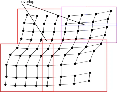
Lists of target points are transferred to those source processes for which an over-lap has been determined, and a grid hierarchy is established out of the source grid on the source side. For block-structured grids, a coarse grid is easily constructed by sub-sampling the grid points of the source grid. A grid hierarchy is constructed with a

20

refinement factor of two similar to a multi-grid approach until the finest level is reached (see Fig. 2). Bounding boxes are constructed by simply evaluating the minimum and maximum cell extent in a given i-j-k index range. Due to this simple approach, neigh-bouring bounding boxes may overlap. If some target point is located in such an overlap region, the algorithm is prepared to investigate the neighbouring boxes until it is able to

25

(15)

GMDD

2, 797–843, 2009

modelling

R. Redler et al.

Title Page

Tables Figures

◭ ◮

Back Close

Full Screen / Esc

the following steps are only local operations in the grid point space while the costly search on the global domain is already completed with the multi-grid algorithm.

A great advantage of the multi-grid algorithm is that it is only weakly dependent on the problem size. When the grid size is doubled in each horizontal direction this would only introduce one more multi-grid level. For very small problem sizes one may

5

argue that the multi-grid algorithm creates too much overhead and a simple search would be more efficient. For larger grids however, the overhead to set up the multi-grid hierarchy is more than compensated by the speedy search and even allows to handle very large problem sizes (e.g. a global grid with 1/12◦_{horizontal resolution) in a}

reasonable amount of time. We postpone this discussion to Sect. 8.

10

In an intermediate step, the source points are now used to construct an auxiliary cell grid where the source points serve as corners of the cells (see dashed and solid lines in Fig. 3). The next task is to locate the source-point cell which contains the projection of the respective target point. This is performed with a local search by investigating each of the four source-point cells that surround the point which belongs to the marked

15

source cell. In this example, the source-point box built with points at indices [i,j], [i+1,j], [i,j+1], and [i+1,j+1] is chosen and the source-cell of the point [i+1,j+1] (green box in Fig. 3) is found. This immediately directs us to identify the point with index [i,j] as the “lower-left” source-point. This location is now stored as the reference location for the particular target point. In a third step, the remaining neighbours are identified which are

20

required to perform the interpolation requested by the user. For a bilinear interpolation, we are now able to identify the four corner points of the auxiliary cell (black open and solid bullets connected by solid lines) as the four neighbour source points needed. For a bicubic interpolation, sixteen neighbours have to be identified (the aforementioned bilinear points plus the open blue circles shown in Fig. 3).

25

(16)

GMDD

2, 797–843, 2009

modelling

R. Redler et al.

Title Page

Tables Figures

◭ ◮

Back Close

Full Screen / Esc

neighbour points are available for the interpolation as they are masked out and the physical fields do not necessarily contain meaningful values on those points. The user API provides different choices to the user via the XML file in such cases. As a default option, the remaining valid points will be used for a weighted-distance interpolation. As an alternative, the choice is provided to not interpolate onto such target points. In

5

the extreme case when all neighbour source points identified by the default search are masked, OASIS4 offers the possibility to search for the non-masked nearest-neighbour value and use this value for the target point. For this extra nearest-neighbour search, the algorithm starts from the original masked source grid point taken as an initial guess. Starting from the finest level containing the initial guess, the multi-grid hierarchy is then

10

used again to locate the closest non-masked source points by moving in so-called w-cycles through the multi-grid hierarchy, that is going down to a coarser level and going up again into another branch of the hierarchy repeatedly until the closed point is found.

5.2 Search on domain-partitioned source grids

On modern parallel systems, the application domain is in general distributed to many

15

processes and/or processors. If the interpolation of fields is performed using locally available data only, i.e. data which is available on the actual process, the result of the interpolation may depend on the actual partitioning. For example, if a target point is located close to the internal border of a partitioned domain of the source application, the standard interpolation stencil may require source points which are not located on

20

the actual process but which are located on a neighbour process. In such a case, the OASIS4 coupler provides the possibility to use only locally available data or to use also the data of other process domains for the interpolation. In the first case, the interpola-tion result (and thus the result of the entire simulainterpola-tion) will depend on the partiinterpola-tion of application domains; in the second case, the interpolation result is independent of the

25

partitioning. In the OASIS4 context, the latter approach is called global search.

(17)

lo-GMDD

2, 797–843, 2009

modelling

R. Redler et al.

Title Page

Tables Figures

◭ ◮

Back Close

Full Screen / Esc

cal interpolation data to the OASIS4 coupler. Since the definition of application grids is quite general and since the full connectivity information for partitioned grids is not provided to the OASIS4 library (and is not explicitly available in most of today’s climate model component codes), missing source points for interpolation stars require an ad-ditional search step. In this adad-ditional search step, the missing source points for the

5

interpolation are searched in neighboured domains. For block-structured grids, neigh-bouring domains are identified by exchanging information about the global index space which is derived using the information provided through the PRISM Def Partition func-tion call. If these source points are found, the full informafunc-tion including the mask data are returned to the process which has initiated this additional search step. This

pro-10

cess collects the data from possibly di_fferent processes and forwards the data for the full interpolation to the coupler.

5.3 Point-based search for Gauss-reduced grids

Gauss-reduced grids have been introduced mainly for atmospheric models in particu-lar the ARPEGE and IFS models (see e.g. D ´equ ´e et al., 1994) to overcome problems

15

resulting from the convergence of meridians close to the geographical poles. As these models and grids play an important role for the atmospheric modelling community, the decision has been made to support this type of grid as a special case. These grids cannot be classified as block-structured grids, nor are they completely unstructured. So instead of treating them as unstructured grids, we are in this particular case able to

20

make use of some implicit knowledge about how the grid is constructed and introduce an intermediate step. In order to reuse as many of the existing functions as possible, we set up an block-structured auxiliary grid which is regular in longitude and latitude and determine the corresponding mapping of the Gauss-reduced grid points onto this auxiliary grid. We are now able to perform the initial search on the auxiliary grid and

de-25

(18)

GMDD

2, 797–843, 2009

modelling

R. Redler et al.

Title Page

Tables Figures

◭ ◮

Back Close

Full Screen / Esc

to block-structured grids, the connectivity cannot be derived from the i–j indices directly. Instead we have to determine the connectivity among the grid points stored in an 1-D array in order to proceed with the local search; this is done based on the description of the Gauss-reduced grid provided by calling the routine PRISM Reducedgrid Map in the component code.

5

5.4 Cell-based search

Compared to the search described above for point-based interpolation schemes, the cell-based search has to follow a slightly different approach. In order to determine all necessary information for conservative remapping, the task here is to locate for each target cell its overlapping source cells. In order to again reuse as many functionality

10

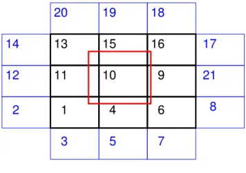
as possible, we perform a point-based search on the corner coordinates in a very similar way to the search described above up to the point where we have obtained the start location. These indices still refer to the data structure of the corner points; with block-structured grids, they can easily be mapped to cell indices, with each cell e.g. described by its four corners. For each target cell (see Fig. 4), we can now use

15

this initial source cell to continue the local search and identify the remaining source cells which overlap a given target cell. The intersection or overlap between a pair of source and target cells is determined by a pairwise investigation of the intersection of the edges without a detailed evaluation of the exact area of overlap. The numbering shown if Fig. 4 indicates the order in which the local search is performed on the source

20

grid. In this particular case 21 cells are investigated starting with the initial source cell 1. For each of the source cells the overlap with the target cell is checked. Source cells with no overlap are marked as visited. Source cells that overlap with the target cell are marked and stored in memory. For an individual local search, the path way through the source cells is not fixed but dependent on the local problem.

(19)

GMDD

2, 797–843, 2009

modelling

R. Redler et al.

Title Page

Tables Figures

◭ ◮

Back Close

Full Screen / Esc

5.5 Optimisation

Most grids used in Earth system modelling are block-structured grids. Historically, codes have been developed with non-global grids in mind and more important, for stand-alone models. Particular issues regarding the connectivity are handled internal to the code to the extend it is needed to provide all information for the advection and

5

diffusion operators and other boundary conditions. For global grids so-called cyclic boundary conditions have been introduced to guarantee a seamless continuation of the grid in the zonal direction. When approaching the geographical poles additional ghost-cells are introduced in order to properly calculate the operators along the zonal boundaries (see e.g. Madec and Imbard, 1996). When considering the i–j domain in

10

the case of coupling, a remote cell close to the pole may extent further than what is covered by the ghost-cell in the i–j space. As the codes lack the information about the connectivity at the poles in general an additional search in the geographical domain is necessary. If the application is able to provide information about the connectivity in an explicit way, a new interface routine could be added to the API to transfer it to

15

the PSMIle. This will help to increase the e_fficiency of the search locally and across process boundaries beyond what is achieved already today.

The OASIS4 PSMILe search algorithms are designed to work on 3-dimensional model domains. In general, one could think about treating all grids as 3-dimensional fully irregular or unstructured grids. In this way one would ignore important a-priory

20

information useful to speed up the search process. In order to take advantage of the existing a-priory knowledge (in particular about regularity along any of the grid axis) different grid types are introduced. The different vertical layers of grids with vertical z-coordinates are usually a simple vertical translation of the same 2-dimensional hor-izontal grid. In such cases, the search is split into two parts with a 2-dimensional

25

(20)

con-GMDD

2, 797–843, 2009

modelling

R. Redler et al.

Title Page

Tables Figures

◭ ◮

Back Close

Full Screen / Esc

ducted by performing a 1-dimensional search along each axis which further reduces the compute time.

It is obvious that individual source cells or source points are needed for more than just one target location. In order to minimize the amount of data to be transferred and stored, redundant geographical information (usually of type double precision or real)

5

is removed and an index list is created which points to the required source data for each target location. These lists (data and indices) are transferred to the Transformer process for further processing.

6 PSMILe-transformer interaction and regridding

As outlined further in Sect. 7, the PSMILe supports two different ways of exchanging

10

data, directly between two components or through the Transformer processes when regridding is required. Here we concentrate on the latter case and describe the transfer of information between the PSMILe and the Transformer and the regridding per se done on the coupling fields.

As the final result of the PSMILe search described in the last section, each source

15

process holds 1-dimensional lists about the source neighbour points required for the regridding of the target points encompassed by its local domain; the information rele-vant for the intersection of the local source grid domain with each target process grid domain is stored in a particular list. Along with the raw geographical information, index lists are created to guarantee a well defined and correct access to the data. In order

20

to allow the scattering onto the final n-dimensional destination array during the data exchange, index lists are transmitted to the target process.

The lists containing the geographical information and the access information are equally distributed over the number of Transformer processes available, resulting in an effective parallelisation of the Transformer over these lists. The different Transformer

25

(21)

GMDD

2, 797–843, 2009

modelling

R. Redler et al.

Title Page

Tables Figures

◭ ◮

Back Close

Full Screen / Esc

well defined sequence of actions matching the actions on the PSMILe side. During the initialisation phase, the Transformer processes thereby receives and stores the different sets of lists containing the source and target information required to perform the regridding. During the exchange phase, each Transformer process receives from the source PSMILe the grid point field values (transferred from the source component

5

code with a PRISM Put call) corresponding to its lists, calculates the regridding weights if it is the first exchange, and applies the weights. The resulting target values are made available to the corresponding target PSMILe process. The data are sent upon request from the respective target process (i.e. when a PRISM Get is called in the target component code).

10

The calculation of the weights depends on the regridding algorithm chosen by the user in the XML configuration file which can be different for each coupling field. The current version of OASIS4 supports purely 3-dimensional regridding (3-D n-neighbour distance-weighted average or trilinear interpolation) and 2-dimensional regridding in the horizontal plane (2-D n-neighbour distance-weighted average, bilinear, bicubic

in-15

terpolation or conservative remapping) followed by a linear interpolation in the vertical. As in OASIS3, the 2-D algorithms are taken from the Spherical Coordinate Remapping and Interpolation Package (SCRIP) library (see e.g. Jones, 1999). In particular, for the 2-D conservative remapping, the contribution of each source cell is proportional to the fraction of the target cell it intersects; this ensure local conservation of extensive

20

properties such as fluxes. The 3-D algorithms are 3-D extensions of the 2-D SCRIP al-gorithms. For a detailed description of the regridding the reader is therefore referred to Jones (1999) and to the SCRIP User’s Guide (see Jones, 2001). As the SCRIP bicubic algorithm is based on the function gradient in the i and j directions, it cannot be applied for the Gauss-reduced grids. For those grids, the SCRIP functionality has therefore

25

(22)

ob-GMDD

2, 797–843, 2009

modelling

R. Redler et al.

Title Page

Tables Figures

◭ ◮

Back Close

Full Screen / Esc

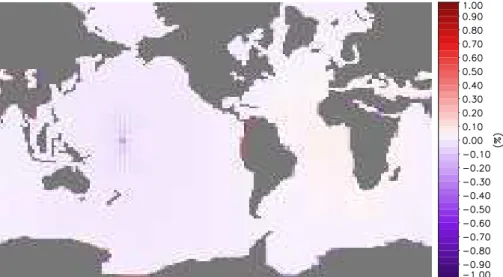
tained when regridding the values of an analytical cosine bell function which presents one minimum and one maximum over the global Earth domain:

F₁₌2−cos[π∗acos(cos(θ)cos(φ))]

The relative error, i.e. the difference between the regridded value and the analytical value of the function divided by the analytical value, is calculated on each target grid

5

point. The Figs. 5 to 8 present the results with each pixel showing exactly this rela-tive error for each grid point. No projection in the latitude-longitude space has been performed to avoid any additional interpolation performed by the graphic package.

Figure 5 shows the relative error obtained with the bilinear interpolation from the LMDz grid to the ORCA2 grid. LMDZ (Hourdin et al., 2006) has a regular

10

3.75◦

×2.535◦grid. ORCA2 (Madec, 2008) is based on a 2◦Mercator mesh, (i.e. vari-ation of meridian scale factor as cosine of the latitude); in the Northern Hemisphere the mesh has two poles so that the ratio of anisotropy is nearly one everywhere. The error is not shown for masked target points (grey areas). One can observe a relative error smaller than 0.4% over the whole domain except near the coastline, for

exam-15

ple near the west coast of the northern South America, where it can reach 0.8% at maximum. For those points near the coastline, some source points that are identified as bilinear neighbours are masked out. The remaining (non-masked) valid points are used for a less precise weighted-distance interpolation resulting in a larger error.

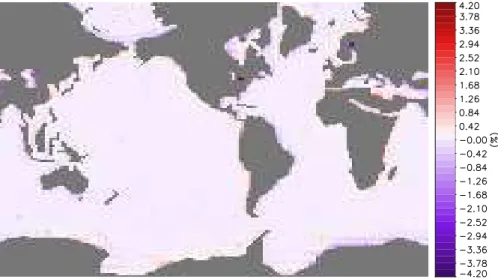
Figure 6 shows the relative error obtained with the bicubic interpolation from a BT42

20

Gauss-reduced grid (with 6232 grid points in total distributed over 64 longitudinal cir-cles) to the ORCA2 grid. The relative error in the equatorial and tropical regions of the basins is smaller than 0.4%, and growing slightly but not above 0.8% at higher or lower latitudes which corresponds to regions where the Gaussian grid is effectively reduced. Again, the error is larger near the coastline, reaching even about 4.2% for some points;

25

(23)

GMDD

2, 797–843, 2009

modelling

R. Redler et al.

Title Page

Tables Figures

◭ ◮

Back Close

Full Screen / Esc

Figure 7 shows the relative error obtained with the conservative remapping from the ORCA2 grid to the LMDz grid. The relative error is everywhere smaller than 0.2% except for the last row of the LMDz grid close to the North pole and near the coastline where it can reach respectively 1% and 2.2%. The SCRIP library assumes that the border of a cell between two cell corners is linear in longitude and latitude: near the

5

North pole, this assumption becomes less valid and this can explain the larger error. Near the coastline, different normalisation options are available in the SCRIP library to calculate the value of the target cells which partially overlap masked source cells (see Jones, 2001). We chose the option to normalize by the area of the target cell intersecting non-masked source cells; this option does not locally conserve extensive

10

properties but results in more realistic target values even if the error is still relatively large. With the alternative option, the normalisation by the full area of the target cell, the relative error observed (not shown) can become as large as 100%.

We note here that as the data structure that is provided to the OASIS4 Transformer differs from the data structure sent to the OASIS3 Transformer, truncation errors may

15

therefore lead to slight differences when comparing the results obtained with OASIS3 and with OASIS4 even though both software use the same regridding algorithms.

Finally, as an illustration of the benefits of the global search (see Sect. 5.2), Fig. 8 shows the relative error obtained with the bilinear interpolation from the LMDz grid to the ORCA2 grid when each component is partitioned over 3 processes (in the

longi-20

tudinal direction) and when the global search is not activated. Comparing with Fig. 5, we observe greater relative error (of the order of 1% comparable to the maximum error obtained near the coastline) near the borders of the source partitions. This can be ex-pected as the local search cannot, for those target points find the usual 4 surrounding neighbours needed for the bilinear interpolation (as some of those 4 are in fact located

25

(24)

GMDD

2, 797–843, 2009

modelling

R. Redler et al.

Title Page

Tables Figures

◭ ◮

Back Close

Full Screen / Esc

not partitioned cases, which validates the global search.

7 Data exchange

The exchange of coupling data is typically happening inside a loop over time or itera-tions and is invoked many times during the execution of the coupled model. Therefore the handling of the data exchange is a time-critical task. One of the major targets is to

5

minimise the communication overhead and to avoid load-balancing problems induced by the implementation of the exchange.

The data exchange is invoked by the component models using the PRISM Put and PRISM Get interface routines. As described in Sect. 4.2, the routines can be used to read from and write to NetCDF files as well as sending data to and receiving data

10

from another model component. The arguments of the subroutine calls are identical for IO and coupling operations, and the concrete action(s) are only specified in the component XML configuration file.

Figure 9 schematically illustrates possible communication pathways in a coupled ap-plication including the access of data from files. Depending on the respective grid

15

configuration, the exchange of coupling data is handled in two different ways. Data points that reside on identical geographical locations on the source and target side are exchanged directly between the component processes (involving repartitioning if necessary). Data points for which a regridding is required are sent through the Trans-former. Matching and non-matching grid points are identified by the PSMILe solely

20

based on the geographical description of the grid. In order to reduce the amount of messages to be exchanged, the current implementation assumes that the number of matching points must at least sum up to 10% of the total number of grid points. For any number below this threshold, matching data are exchanged together with non-matching data through the Transformer processes. To further optimise the exchange of data and

25

(25)

GMDD

2, 797–843, 2009

modelling

R. Redler et al.

Title Page

Tables Figures

◭ ◮

Back Close

Full Screen / Esc

onto the destination array behind the PRISM Get call and provided to the API in the appropriate array shape leaving masked target indices untouched. The calculation of regridding weights in the Transformer is delayed until the first exchange for which a particular set of weights is required. The weights are then stored in the Transformer for subsequent exchanges.

5

It noteworthy to mention that the data are buffered internally on the sender side and transferred with a so-called non-blocking MPI function (MPI Isend). This guarantees that the PRISM Put will immediately return when the data are stored locally even if the target component (be it the Transformer or another component in case of direct com-munication) is not yet ready to receive data. On the sender side the user code outside

10

the PSMILe can safely progress and reuse its own local memory. The PRISM Get on the other hand will only return when the data are received.

The IO layer is based on the mpp io package as described by Balaji (2001). For the OASIS4 PSMILe IO, various modes are supported which become especially relevant if components are parallelised. The default behaviour of the PSMILe is, for output,

15

to collect all data on the component root process and write out data into a single file or, for input, to read data on the component root process and distribute it internally. While this approach is still applicable when the domain partitioning is changing from job to job (especially when thinking about coupling restart files) it may not be the most performant way to deal with the IO. As an alternative approach, all IO processes read

20

data from and write data to individual files. For further analysis these files have to be glued together in a postprocess. In order to support a full parallel IO, the mpp io package has been extended to be compliant with the pNetCDF library (Li et al., 2003). When linked against pNetCDF, data are written into and read from a single file via MPI-IO with no pre- or postprocessing required. From a user perspective, this approach is

25

invariant to changes in domain partitioning and should also provide a reasonable IO performance provided that the respective MPI-IO implementation efficiently uses the underlying system architecture (memory layout and file system).

(26)

trans-GMDD

2, 797–843, 2009

modelling

R. Redler et al.

Title Page

Tables Figures

◭ ◮

Back Close

Full Screen / Esc

formation routines like time-accumulation, time-averaging, gathering and scattering of physical fields and performs the required transformation locally on the source side be-fore the exchange with other components of the coupled system or IO; only the end product is then communicated to the target.

8 Performance

5

Regarding the general performance of the coupling software from a user point of view it is tempting to ask for an exact number concerning the cost of the coupling and the overhead the user has to pay in terms of CPU seconds or a percentage of time. For full ESMs, it is difficult to predict the additional time needed for the coupling. To some degree, this depends on the search that has to be performed on a variety of grids for a

10

larger number of exchange fields and di_fferent regriddings. Another important aspect is the run-time behaviour of the different ESM components and the load-(im)balancing between the processes involved. This may strongly influence the time needed to per-form a data exchange. ESMs di_ffer from each other in the above mentioned aspects, and providing a number for a particular ESM is of little help and not in the scope of

15

this article. In addition, the picture may again change completely when an ESM job is running in batch mode and eventually has to share some resource with competing applications. In the following, our aim is to give a first idea about the potential cost for coupling and to provide information about the efficiency of the coupling software as such. Therefore we try to exclude the aforementioned side e_ffects as much as possible.

20

(27)

GMDD

2, 797–843, 2009

modelling

R. Redler et al.

Title Page

Tables Figures

◭ ◮

Back Close

Full Screen / Esc

8.1 Benchmark design

Here we investigate the so-called “strong scaling” properties of OASIS4. By keeping the global problem size constant, we expect a decrease in CPU time for individual pro-cesses with the problem distributed to larger number of propro-cesses in proportion to the local problem size. While this is in general reflecting the typical situation the user is

5

confronted with, strong scaling is considered to be more difficult to achieve (in contrast to weak scaling where the local problem size is kept constant and the global problem to be solved is increased with increasing numbers of processes used). The test case we are considering now is a bidirectional exchange of 2-dimensional data between a global T255 “atmospheric” grid for component A and an “ocean” grid with 0.3◦

×cosφ

10

horizontal resolution for component B, ranging from 0◦_{to 360}◦_{in longitude and latitudes}

φbetween 70◦_{S and 70}◦_{N. This corresponds to 1202×665 grid points for component B}

and 768×385 grid points for component A. Both grids are described as horizontally ir-regular grids in order to bypass the optimised routines that are available for completely regular grids and to mimic the large class of use cases, the 2-dimensional data

ex-15

change between any two physical components at the Earth surface. Some of the ocean and atmosphere grid points have been masked out in order to bypass additional opti-misation steps of the search algorithm which can be applied if complete non-masked grids are treated. The search is performed for bilinear interpolation without requesting an extra nearest-neighbour search for target points that only have masked “bilinear”

20

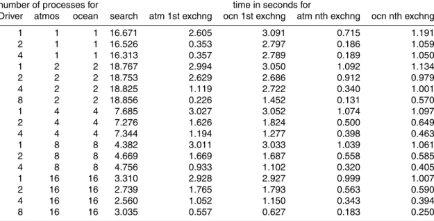
source points (see Sect. 5.1). The search is performed for one exchange field for each direction. In an additional test, we have expanded the search problem into the vertical dimension towards a full 3-D-dimensional search and data exchange with 40 levels for component A and 45 levels for component B.

For this particular benchmark calculations, the OASIS4 sources have been compiled

25

(28)

Gi-GMDD

2, 797–843, 2009

modelling

R. Redler et al.

Title Page

Tables Figures

◭ ◮

Back Close

Full Screen / Esc

gahertz 2x single core AMD Opteron processor 246 and 4 Gigabyte of memory per node connected via a 2 Gigabit Myrinet. For the message passing, we use the Mes-sage Passing Interface Chameleon Glenn’s MesMes-sages (GM) proprietary communica-tion layer (MPICH-GM) provided by Myricom. For all tests, we have used the MPI1 method where all processes have to be started at once (see Sect. 3).

5

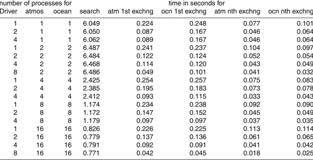
8.2 2-dimensional search

The numbers presented in Table 1 show the wall-clock time needed to perform the search for the bilinear interpolation, the time needed to perform the first exchange of data (which includes the calculation of the weights for the bilinear interpolation in the Transformer), and the time needed for subsequent data exchanges (averaged over

10

100 data exchanges). Although the benchmark has been run on a dedicated system, the numbers in the table only represent snapshots and are subject to slight variance caused by conflicts with system processes. Nevertheless we have not performed any ensemble means with appropriate statistics as this will not change the general picture we are going to discuss.

15

The time needed for the search can be represented by the time needed for the PRISM Enddef routine. The search is performed on the two sets of source component processes as the component A target points are searched for on the component B processes and vice versa. As the PRISM Enddef and subsequent calls therein contain blocking MPI calls, the total time needed by the PRISM Enddef is to a large extent

con-20

trolled by the source process which has to solve the largest problem (mainly determined by the number of target points to be processed). The time spent in PRISM Enddef is almost identical for all processes due to this blocking nature of the MPI function calls used inside. Therefore only one number, the time needed by the component process with the largest data load is shown in the table for each setting. For the first and

25

subsequent data exchanges, the time is provided for the slowest component process, separately for A and B .

(29)

GMDD

2, 797–843, 2009

modelling

R. Redler et al.

Title Page

Tables Figures

◭ ◮

Back Close

Full Screen / Esc

processes dedicated to the components: in this case, the speed-up is roughly a factor of 7 when going from 1 to 16 processes. When going from one to two component pro-cesses, the time for the search is slightly increased. The main reason can be attributed to the different algorithms used, as in the one-processor case certain subroutines do not have to be called simply because no boundary exchange is required on the source

5

grid. When the number of processes is increased further the required wall-clock time is reduced significantly to values well below 1 s for the 2-D data exchange on 16 proces-sors. At this stage, the number of Transformer processes is not of critical importance as they are not involved in the search as it is only at the very end of the search cycle that results are delivered to the Transformer process(es) (see Sect. 6).

10

8.3 2-dimensional data exchange

In this example, a data exchange can be understood as one pair of PRISM Put and PRISM Get operations in each component (referred to as ping-pong). The time needed for a complete ping-pong usually is different on each process. Load-balancing prob-lems provide only one answer to explain this behaviour, and is beyond the control of

15

the PSMILe. Furthermore, it may happen that one instance of the coupled system may have to receive more than just one message at a time. This is e.g. the case if only one Transformer process is available and two source components are trying to send or receive data at the same time. In this case, the messages can only be processed one after the other by the Transformer causing other component processes to wait. As only

20

non-masked data are exchanged between the components, data are subsampled prior to the send operation and have to be scattered on the receiver side before they are de-livered to the user space. This requires additional operations which are also captured by our time measurements for the ping-pong. In order to provide only a single number for the ping-pong, we show the time needed by the slowest component processor to

25

complete the exchange.

(30)

GMDD

2, 797–843, 2009

modelling

R. Redler et al.

Title Page

Tables Figures

◭ ◮

Back Close

Full Screen / Esc

is that the likelihood of the Transformer process being ready to receive, process and send data increases. The other reason is that the amount of data to be treated is re-duced for each process. The only case when increasing the number of Transformer processes does not result in a decrease of the exchange wall-clock time is when the components themselves are not parallel and when the number of processes for the

5

Transformer goes from 2 to 4. In this case, as the components are not parallel, there are only two distinct lists of source neighbour points required for the regridding of target points, i.e. one when considering component A as the target and one when consider-ing component B as the target. As the Transformer is parallelised over these lists (see Sect. 6), the 2 additional processes (when going from 2 to 4 processes) do not get any

10

workload and do not participate in the data exchange.

During the first exchange of data in addition to the processing of the exchange fields, the Transformer has to calculate the weights which are then stored and reused for subsequent data exchanges. This additional workload is responsible for the longer time needed to perform the first exchange when comparing with the time needed for

15

subsequent exchanges.

It can also be observed that for a fixed number of Transformer processes the ex-change time is fairly independent of the number of application processes. As the data are exchanged through the Transformer processes, it can act as a bottleneck in the exchange if it is not sufficiently parallel. In general, it is the number of available

Trans-20

former processes that dictates the speed of the exchange and not the parallelisation of the components themselves.

Finally, one can also observe that the scaling behaviour is in general not fully pre-dictable; this can mainly be attributed to the fact that a particular Transformer process may still be busy with other tasks, that data are sometimes not available from the

25