Next generation framework for aquatic modeling of the Earth System

(1)

GMDD

2, 279–307, 2009

NextFrAMES

B. M. Fekete et al.

Title Page

Abstract Introduction

Conclusions References

Tables Figures

◭ ◮

Back Close

Full Screen / Esc

Printer-friendly Version

Interactive Discussion

Geosci. Model Dev. Discuss., 2, 279–307, 2009 www.geosci-model-dev-discuss.net/2/279/2009/ © Author(s) 2009. This work is distributed under the Creative Commons Attribution 3.0 License.

Geoscientific Model Development Discussions

Geoscientific Model Development Discussionsis the access reviewed discussion forum ofGeoscientific Model Development

Next generation framework for aquatic

modeling of the Earth System

B. M. Fekete1,*, W. M. Wollheim2, D. Wisser2, and C. J. V ¨or ¨osmarty1,*

1

CUNY Environmental Cross-roads Initiative, The City College of New York at the City University of New York, 160 Convent Avenue, New York, New York, 10031, USA

2

Complex Systems Research Center, Institute for the Study of Earth, Oceans and Space, University of New Hampshire, 39 College Rd., Durham, 03824, USA

*

also at: NOAA-Cooperative Remote Sensing Science and Technology Center, The City College of New York at the City University of New York, 160 Convent Avenue, New York, New York, 10031, USA

Received: 24 February 2009 – Accepted: 4 March 2009 – Published: 17 March 2009

Correspondence to: B. M. Fekete (bfekete@ccny.cuny.edu)

(2)

GMDD

2, 279–307, 2009

NextFrAMES

B. M. Fekete et al.

Title Page

Tables Figures

◭ ◮

Back Close

Full Screen / Esc

Abstract

Earth System model development is becoming an increasingly complex task. As sci-entists attempt to represent the physical and bio-geochemical processes and various feedback mechanisms in unprecedented detail, the models themselves are becoming increasingly complex. At the same time, the complexity of the surrounding IT

infras-5

tructure is growing as well. Earth System models must manage a vast amount of data in heterogeneous computing environments. Numerous development efforts are on the way to ease that burden and offer model development platforms that reduce IT chal-lenges and allow scientists to focus on their science. While these new modeling frame-works (e.g. FMS, ESMF, CCA, OpenMI) do provide solutions to many IT challenges

10

(performing input/output, managing space and time, establishing model coupling, etc.), they are still considerably complex and often have steep learning curves.

The Next generation Framework for Aquatic Modeling of the Earth System (NextFrAMES, a revised version of FrAMES) have numerous similarities to those developed by other teams, but represents a novel model development paradigm.

15

NextFrAMES is built around a modeling XML that lets modelers to express the over-all model structure and provides an API for dynamicover-ally linked plugins to represent the processes. The model XML is executed by the NextFrAMES run-time engine that parses the model definition, loads the module plugins, performs the model I/O and executes the model calculations. NextFrAMES has a minimalistic view representing

20

spatial domains and treats every domain (regardless of its layout such as grid, network tree, individual points, polygons, etc.) as vector of objects. NextFrAMES performs computations on multiple domains and interactions between di_fferent spatial domains are carried out through couplers. NextFrAMES allows processes to operate at different frequencies by providing rudimentary aggregation and disaggregation facilities.

25

(3)

GMDD

2, 279–307, 2009

NextFrAMES

B. M. Fekete et al.

Title Page

Tables Figures

◭ ◮

Back Close

Full Screen / Esc

Earth System models, but future versions with the guidance from Earth System de-velopers might someday eliminate its limitations. Our intent with NextFrAMES is to initiate a dialog about new ways of expressing models that is less tied to the actual implementation and allow scientist to develop models at a more abstract level.

1 Introduction

5

Earth System modeling is an increasingly challenging task due to the rapidly increas-ing complexity of the models themselves (Hall and O’Connell, 2007). Modern land surface, ecosystem, hydrological, etc. models represent biogeochemical and physical processes in such detail that model codes become very complicated. In addition to the complexity of the models themselves, the IT infrastructure upon which the

mod-10

els are built is growing more complex as well. While both computational power and mass storage media capacity have undergone exponential growth following Moore’s law, the speed of accessing the mass storage devices clearly lagged behind. As a consequence, applications today are often limited by the read and write access of the vast amount of data required by the models. One way to reduce the limitations of slow

15

storage devices is to trade data storage for processing on the fly. For instance, down-scaling algorithms built into models can reduce the amount of data that the models need to read. However, this solution comes at the price of performing computationally intensive interpolation algorithms as part of the model simulations. Such an approach essentially makes the already complicated models even more complex.

20

To complicate the matter further, the efficient management of the vast amount of data available to Earth Scientists requires sophisticated solutions. The era of “ad hoc” input/output using primitive, home-grown data formats is over; scientific data need a common management framework that provides catalogs, documentation, discovery mechanisms and preprocessing to feed the scientific applications. While emerging

25

(4)

GMDD

2, 279–307, 2009

NextFrAMES

B. M. Fekete et al.

Title Page

Tables Figures

◭ ◮

Back Close

Full Screen / Esc

already complex models.

When one considers that the computational power of single CPU core has remained more or less steady over the last four years while the Moore’s law was realized by adding more cores to the CPUs (dual and quad core CPUs becoming common even in ordinary desktop computers) the need for implementing Earth System model

com-5

ponents in a parallel processing environment is inevitable. Furthermore, parallel com-puters have vastly different architectures ranging from symmetric memory processing (SMP, when multiple processors have access to the same memory), non-uniform mem-ory access (NUMA, when processors have access to faster memmem-ory individually and share common access to slower memory units) and cluster computers (e.g. Beowulf,

10

when entire computers are clustered via fast network connections). These different platforms need very different parallelization strategies.

Computer science has delivered numerous essential components to make the uti-lization of these different architectures easier. For instance, Message Passing Inter-face (MPI) is commonly used in many parallel applications. No new development

15

platform has emerged yet that could help to automate the parallelization of scientific tasks. When parallel computers became commonplace more than twenty years ago, one would have thought that new “non-procedural” languages (like LISP or Prolog) would emerge allowing the description of the computational tasks in a conceptual man-ner that intelligent interpreters or compilers could analyze and optimize to execute on

20

parallel CPU systems. The last two or three decades brought numerous new program-ming languages into play (C++, Java, Python) and new concepts like structured and object oriented programming. The new languages primarily aided the construction of complex applications by compartmentalizing the application development and allowing higher levels of modularity, but these languages remained “procedural” in the sense

25

(5)

GMDD

2, 279–307, 2009

NextFrAMES

B. M. Fekete et al.

Title Page

Tables Figures

◭ ◮

Back Close

Full Screen / Esc

are rarely suitable for Earth System models.

The lack of new development concepts might be due to the large differences in them demands of specific applications, so no common solution has yet emerged. As a con-sequence, we argue that Earth Scientists need to develop their own model develop-ment platform that is designed to address Earth Science problems. This new model

5

development platform needs to be built on a new paradigm that allows the description of scientific tasks in a hardware platform independent manner.

1.1 Existing modeling frameworks

The need for unified modeling frameworks was realized long time ago and numerous solutions are emerging with different design goals. While all modeling frameworks are

10

aimed at simplifying the integration of model components one way to categorize them might be the level at which the model integration occurs. The Flexible Modeling Sys-tem1(FMS, developed at the Geophysical Fluid Dynamics Laboratory, GFDL) and the Earth System Modeling Framework2 (ESMF, which might be viewed as descendant of FMS, was originally initiated by NASA, and currently under development at NCAR)

15

both provide a series of utilities and services to model developers in the form of func-tion libraries that provide solufunc-tions to various computafunc-tional demands. ESMF offers function library tools for handling components (primarily grid) and associated arrays of variables, partitioning of components for execution on multiple processors, distribu-tion of data to processors, exchange of data between processors and the gathering

20

calculation results, management of time stepping, data exchanges between di_fferent components (coupling), input/output and log facilities. ESMF can be used as a primary mean for managing space and time in an Earth System model or it can be used as a wrapper around existing models that otherwise have their entirely di_fferent internal structure.

25

1

http://www.gfdl.noaa.gov/∼fms

2

(6)

GMDD

2, 279–307, 2009

NextFrAMES

B. M. Fekete et al.

Title Page

Tables Figures

◭ ◮

Back Close

Full Screen / Esc

While ESMF can be used as a “glue” between different models, its primary goal is to provide unified internal model infrastructure. In this respect, ESMF is a huge step forward as a new hardware-independent modeling platform, but the use of ESMF still has steep learning curve and requires the model developer to deal with low-level details (e.g. partitioning the model domains into computational subregions, managing the data

5

distribution between compute nodes, etc.).

Open Modeling Interface3 (OpenMI) funded by the European Commission and the Common Component Architecture4 (CCA) initiated by the U.S. Department Energy provide solutions to higher level model coupling. Both OpenMI and CCA are designed to couple entire models (just like when ESMF is used in a “glue wrapper” mode. The

10

capability to couple entire models is certainly useful, particularly the wrapping existing models into a larger modeling infrastructure, but at some point the legacy models will have to be retired as computer hardware and the software infrastructure makes them obsolete.

Perhaps the biggest shortcoming of coupling entire models is that as soon as these

15

models maintain their own way of managing space and time (and consequently perform input/output in their own way), the necessary wrapper environment to handle the model differences needs to be fairly complicated. Furthermore, space and time management are exactly the most critical elements for parallel execution, so once they are embed-ded deeply in the model, any support to aid parallelization, and computational load

20

balancing from the modeling framework standpoint becomes difficult if not impossible. A third set of popular modeling environments came from commercial software ven-dors such as Matlab5, S-Plus6 (and its open source equivalent R7), Stella, Simile8

3

http://www.openmi.org

4

http://www.cca-forum.org

5

http://www.mathworks.com

6

http://www.insightful.com

7

http://www.r-project.org

8

(7)

GMDD

2, 279–307, 2009

NextFrAMES

B. M. Fekete et al.

Title Page

Tables Figures

◭ ◮

Back Close

Full Screen / Esc

(Muetzelfeld and Masshender, 2003) and COMSOL9. These are probably the tools that are the closest to the new model development platforms that Earth system scientists will need. Actually, numerous Earth System model components have implementation using these tools (e.g. Topmodel written in Matlab, etc.). The common service that these tools provide is a simple means to perform computation with different levels of

5

complexity on variable arrays, so that developers could focus on the actual compu-tational tasks and let the software to perform rudimentary data management. While these software development platforms are often extremely valuable for quick prototyp-ing, they don’t scale well to the massive computational tasks of large Earth System models. Furthermore, these software tools are rarely geared to Earth science needs

10

and due to the closed source nature of commercial software, adding the needed ex-tensions is rarely feasible.

1.2 Common Earth System model function

The most important common functions that Earth System models and model compo-nents share is the discretization of space and time, linkages between different

compu-15

tational domains that discretize space and time di_fferently (coupling) and calculations on the discrete spatial objects at some computational frequency. The discretization of time is perhaps more trivial since it is only a one dimensional problem and the major challenge is to map the regular time intervals to the somewhat irregular time incre-ments in traditional calendars (e.g. varying length of month, leap years, the disconnect

20

between weekly and monthly increments). A discretization of space is more challeng-ing. Numerous solutions to numerically represent spatial features have emerged over the last few decades. The three characteristically different approaches are Geographi-cal Information Systems, remote sensing image processing systems and Earth System Model tools. The primary focus of traditional GIS was to represent static spatial

fea-25

tures via series of contours and polygons. Representing similar features in a gridded

9

(8)

GMDD

2, 279–307, 2009

NextFrAMES

B. M. Fekete et al.

Title Page

Tables Figures

◭ ◮

Back Close

Full Screen / Esc

context was added later as a mean to make overlay calculations easier. The line be-tween gridded GIS and image processing is blurry, but the biggest difference perhaps is that image processing tools need to manage not only static images, but the also changes that occur over time, yet typically at low temporal frequency (often in the order of daily to bi-weekly intervals). Earth system model tools (which don’t really have a

5

name on their own, but can be regarded as the tools supporting NetCDF10 developed mostly by NCAR) were designed to manage space and time at high temporal frequen-cies by compromising on spatial resolution. These tools treat three or four dimensional arrays (representing 2D or 3D domains in time) as single objects.

The synergy of the GIS, image processing and Earth system tools is critical for the

10

next generation of Earth System models to enable modelers to perform simulations over the computational domains that are most suitable for the particular model com-ponents and yet enable model comcom-ponents (operating on one type of spatial domain layout) to interface with other components. This synergy will require a generalized means of exchanging information between different domains (coupling).

15

1.3 Science expression in Earth System model components

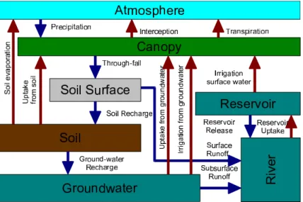
Scientific representation of different Earth System model components often express the model structure in a form of block diagram (Fig. 1). The scientific thinking in these block diagrams have two components a) the block diagram layout and b) the processes in the boxes of the block diagram. An ideal modeling framework would allow scientists

20

to focus on these two and alleviate the need to deal with core model functions such as performing model I/O, handling spatial objects and advancing time, or providing visualization.

This level of abstraction improves the model documentations and serves as the ulti-mate means to plug and play compatibility of model components. While the

implemen-25

tation of space and time management in such a modeling framework might be limiting

10

(9)

GMDD

2, 279–307, 2009

NextFrAMES

B. M. Fekete et al.

Title Page

Tables Figures

◭ ◮

Back Close

Full Screen / Esc

for applications where novel approaches representing both is integral part of the sci-ence (e.g. adaptive finite di_fference meshes) as these technologies mature they could be implemented in the modeling frameworks.

2 Next generation framework for aquatic modeling of the Earth System

We have developed several modeling frameworks (Data, Assembler, FrAMES, and

5

NextFrAMES) in the last 15 years following the previously described design goals. The latest effort building on the Framework for Aquatic Modeling of the Earth System (FrAMES) (Wollheim et al., 2008) was started about a year ago in response to the need identified in the ongoing NASA WaterNet Solution Networks and IDS projects. While FrAMES (as its name implies) was primarily designed to support hydrological

10

and constituent transport and processing models, NextFrAMES eliminates most of its limitations and offer a modeling platform for wide range of land surface modeling applications.

NextFrAMES includes

15

– modeling XML (to describe the overall model structure),

– module plugin Application Programming Interface (API) for C/C++ (future ver-sions of FrAMES will have bindings to other languages),

– I/O plugin API for di_fferent file and data services (OpenDAP, WaterML, etc.)

– run-time engine (currently designed for single CPU system, but we anticipate SMP

20

(10)

GMDD

2, 279–307, 2009

NextFrAMES

B. M. Fekete et al.

Title Page

Tables Figures

◭ ◮

Back Close

Full Screen / Esc

2.1 NextFrAMES model structure

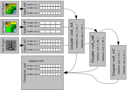
NextFrAMES modeling XML (document type definition provided in Appendix A) orga-nizes models around components (aggregate, container, input, and region (Fig. 2). Components represent spatial domains as a vector of computational objects. The ac-tual handling of the physical domains and the translation from the domain elements

5

(discrete points, grid cells, etc.) to the vector of objects is delegated to I/O plugin in-frastructure. Components maintain lists of variables as a vectors (of the same length as the number of computation objects in the component). Components can contain any number of variables and parameters. Parameters are constant values through space and time.

10

While components themselves have no information about the actual layout (e.g. dis-crete points, grid, gridded networks) of its computational objects, it is the I/O plugin interface that provides the necessary object topologies. An object topology describes the spatial relationships between computational object. For instance, a 2D grid domain could define horizontal and vertical neighbors (2D topology). Gridded river networks

15

(Fekete et al., 2001; V ¨or ¨osmarty et al., 2000) could define downstream and upstream river reach (tree topology). Components could have any number of topologies and the available topologies determine the available spatial operators (derivative, route) the can be requested. Each component has its own temporal frequency at which the component operates.

20

Components can form a hierarchical tree throughcontainer components. Container components hold other components, interfaces and processing modules. Container components inherit their vector of computational objects form other components. Cur-rently onlyinput components can define new vector of computational object.

Aggregate components (Example 2) provide a special means to perform aggregate

25

(11)

GMDD

2, 279–307, 2009

NextFrAMES

B. M. Fekete et al.

Title Page

Tables Figures

◭ ◮

Back Close

Full Screen / Esc

downscale high resolution land-use/cover information into distribution of cover types (as percentages) at a coarser resolution, or calculate aggregate statistics (mean, min-imum, maximum) from fine resolution input to a coarser resolution domain.

Container components (Example 3) are the most important elements of the model definition. Containersprovide the means to exchange variables from one component

5

to another throughinterfaces and hold the modules to perform calculation tasks. An interfacemaps avariablefrom a source component to a newvariablein thecontainer component via coupler. The coupler is a simple weighting mechanism (established by the run-time engine) assigning a set of object from the source component and the cor-responding weighting to a particular object in the destination component (Fig. 2).

Cou-10

plers are one directional, but separate couplers from components can be established in each direction. Establishing couplers is hidden to the modeler and it is NextFrAMES’ duty to find out how to couple two different set of computational objects.

The main purpose of container components to perform computations on the vari-ableswithin the container via process modules provided in dynamically linked plugin

15

(Example 4). Aprocess module plugin (that is written in high level programming lan-guage, currently only in C) has two functions (initialize, execute). Theinitialize function is called in the parsing phase of the model execution. The role of theinitialize func-tion is to return the list of parameters and input and output variables of the module to NextFrAMES. The process modules can define default value and plausible value

20

range11 for each requested parameter. Variables can have default value (to overwrite when missing values occur) and unit attributes. The execute function is called in the model calculation phase for each computational object in thecontainer component re-peatedly for each time step. The NextFrAMES takes care of converting variables to the requested units and place theparametersandvariables into a single user defined

25

11

(12)

GMDD

2, 279–307, 2009

NextFrAMES

B. M. Fekete et al.

Title Page

Tables Figures

◭ ◮

Back Close

Full Screen / Esc

record. The execute functions responsibility is to read the passed variable values and return the results in the output variable elements of the user defined record.

Thevariablesandparametersof aprocessmodule are associated tovariablesand parametersdefined in the container components viaaliases, therefore the same pro-cessmodule can be reused within the same models for di_fferentvariablesand

param-5

eters.

Simplified mechanism to define modules is provided through equations allowing the symbolic definition of calculation within the modeling XML (Example 5). Theequation module usesaliasmechanisms to relate symbolic variables to variablesand parame-tersof thecontainer component.

10

Parameters (that are uniform in space and time during model calculations) can be defined at any level of the components hierarchy down to the module level, which deter-mine the scope of theparameters. For instance,parametersdefined in the “root” con-tainer (which is the model clause of the modeling XML) have global scope (i.e. known throughout the whole model).Parametersdefined in descendentcontainer component

15

are only known within thecontainer and in any of it descendentcontainers.Parameters defined in modules are only known in the module where they were defined.

Derivative and route operator modules (Example 6) perform calculations across topologically linked computational objects. Derivatives calculate forward, backward and center differences in one of the axis direction on 2D or 3D topology. Route modules

20

perform upstream accumulation on objects with tree topology (river network).

Input variables in any module (process, equation, derivative or route) have to be defined before the module is specified. Normally, variables are either defined through interfaces or as outputs from previous modules. Variables that are updated in subse-quent module calculations can be defined asinitial variable. Uniform initial value of the

25

(13)

GMDD

2, 279–307, 2009

NextFrAMES

B. M. Fekete et al.

Title Page

Tables Figures

◭ ◮

Back Close

Full Screen / Esc

The purpose of input components (Example 7) is to translate variables from input sources the vector of computational objects (Fig. 2). An input component uses an I/O plugin to access the content of the input source and retrieve optional object topologies. The I/O plugin is specified in the modeling XML along with the source URL of the external data. Input components can inherit the time step from the input source our

5

specify the input frequency via the “time step” attribute. When the requested frequency is slower than the time step of the input data, the input component performs temporal averaging for the requested frequency. When the input data has lower frequency than the requested time step, the same values are returned at each high frequency data request as a step function. The “offset” attribute (not shown in example) can be used to

10

request low frequency input records in advance or delayed. The o_ffset capabilities will allow the implementation of advanced downscaling (beyond the simple step function) such as bilinear, spline, etc interpolation.

Region components provide a simple means to subset the vector of computational objects, based on simple criteria on a single variable from the source components.

15

For instance, one could implement a plant growth model in NextFrAMES and define bare soil regions (that would vary over time) as a function of vegetation state. Regions actually inherit the layout of the parent component but allow masking inactive objets.

Container components could include outputs requests to write out any variables as the model simulation progresses (Example 8). The output request uses the I/O plugin

20

of the component from which the container inherited its layout (which is always an input component since only input component can define layout).

2.2 NextFrAMES run-time engine

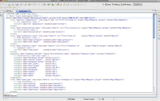
The NextFrAMES run-time engine executes the model components in the order as they are defined in the modeling XML (Fig. 3). Processes defined incontainer component

25

(14)

GMDD

2, 279–307, 2009

NextFrAMES

B. M. Fekete et al.

Title Page

Tables Figures

◭ ◮

Back Close

Full Screen / Esc

for single processor systems. SMP capabilities are anticipated by the end of the 2009. Over time, we would hope to see multiple implementation of the run-time engine to emerge just like there are multiple implementations for web-browsers (Mozilla, Opera, MS Internet Exploder). The different implementation can be optimized for different platforms (ranging from single CPU systems to cluster computers). For instance, an

5

implementation of the NextFrAMES run-time enging for cluster computers could be built on top of ESMF, which already has numerous components needed to manage components with different layouts and couple different domains.

While NextFrAMES is not likely to suit every Earth system model needs, but it cer-tainly can provide a strong basis for a wide range of applications. At the minimum,

10

NextFrAMES is an ultimate “Swiss Army Knife” tool for manipulating time varying spa-tial data products. The ability of interfacing between components at different spatial and temporal frequencies makes NextFrAMES a unique data processing tool that can perform spatial and temporal up and downscaling while performing addition complex calculations. The NextFrAMES modeling XML along with the plugin API has the

po-15

tential to change the model development paradigm similarly to how HTML changed dramatically the sharing and distributing textual content.

3 Conclusions

The main difference between NextFrAMES and existing modeling frameworks is that NextFrAMES is intended to provide a high level abstraction of the scientific tasks in

20

model development and hides largely the common functionality that are targeted by other frameworks.

The NextFrAMES modeling XML and plugin infrastructure provides flexible basis to develop wide range of Earth System model components (land surface, ecosystem and hydrological models). Its operational predecessor (FrAMES) demonstrated the

feasi-25

(15)

GMDD

2, 279–307, 2009

NextFrAMES

B. M. Fekete et al.

Title Page

Tables Figures

◭ ◮

Back Close

Full Screen / Esc

released to the scientific community simultaneously with the publication of the present paper.

The first implementation of the run-time engine that parses and interprets the model-ing XML loads the module and input/output plugins and performs the model simulation is designed for single CPU system, but a parallel version working on shared memory

5

systems is expected by the end of 2009. The parallel and the single CPU implemen-tations of the run-time engine will be able to execute the same modeling XML and corresponding plugins without on single or multi processor machines without modifica-tions. While the current set of input/output plugins are limited to NetCDF data format, additional input/output plugins can be written without affecting the model

implementa-10

tion.

The NextFrAMES run-time engines developed at The City College of New York will be released as open source project through the popular SourceForge archive. The in-tention is to turn NextFrAMES a freely available model development platform that would attract not only model developers to implement their models within the NextFrAMES

in-15

frastructure, but computer scientists to add new features such as data handling capabil-ities to other file formats beyond NetCDF by developing additional input/output plugins or different implementation of the run-time engine optimized from various platforms.

The NextFrAMES modeling platform will provide new opportunities to develop sup-port infrastructure. One can envision graphical model builder graphical interface

(sim-20

ilar to the one in Stella, Simile or Ccaffeine GUI of the Common Component Architec-ture). Additional tools could provide new means to link the models to metadata and data services so the modeler could choose from available input data meeting the in-put requirements of the model simulations and access the data though data services (Horak et al., 2008) (e.g. OpenDAP and OGC WFS data). Surrounding support

in-25

(16)

GMDD

2, 279–307, 2009

NextFrAMES

B. M. Fekete et al.

Title Page

Tables Figures

◭ ◮

Back Close

Full Screen / Esc

Some of the support tools are already under development at The City College of New York supporting and at the University of New Hampshire for both the Global Terrestrial Network for Hydrology (GTN-H, 12) effort of the World Meteorological Organization and the end-to-end water resources management tools developed as CCNY/UNH’s contribution the the State-of-the Global Water Systems initiative of the Global Water

5

Systems Project.

Appendix A

!-- DTD for Land surface model definition file -->

<!ELEMENT model (aggregate|container|input|parameter|region)+> <!ATTLIST model name CDATA #REQUIRED

version CDATA #REQUIRED begin CDATA #REQUIRED end CDATA #REQUIRED>

<!ELEMENT aggregate (category|mean|minimum|maximum|stdev)+> <!ATTLIST aggregate name CDATA #REQUIRED

layout CDATA #REQUIRED component CDATA #REQUIRED variable CDATA #REQUIRED>

<!ATTLIST container name CDATA #REQUIRED layout CDATA #REQUIRED time_step CDATA #REQUIRED states CDATA #REQUIRED>

<!ELEMENT equation (alias|parameter)*> <!ATTLIST equation name CDATA #REQUIRED

equation CDATA #REQUIRED unit CDATA #IMPLIED>

<!ELEMENT input (variable)+> <!ATTLIST input name CDATA #REQUIRED

time_step CDATA #REQUIRED url CDATA #REQUIRED plugin CDATA #REQUIRED method CDATA #REQUIRED>

<!ELEMENT output (variable)+>

12

(17)

GMDD

2, 279–307, 2009

NextFrAMES

B. M. Fekete et al.

Title Page Abstract Introduction Conclusions References Tables Figures ◭ ◮ ◭ ◮ Back Close

Full Screen / Esc

<!ATTLIST output name CDATA #REQUIRED path CDATA #REQUIRED>

<!ELEMENT process (alias|parameter)*> <!ATTLIST process name CDATA #REQUIRED

plugin CDATA #REQUIRED method CDATA #REQUIRED>

<!ELEMENT region (alias)>

<!ATTLIST region name CDATA #REQUIRED condition CDATA #REQUIRED>

<!ELEMENT extent (#EMPTY)>

<!ATTLIST extent direction (x|y|z) #REQUIRED minimum CDATA #REQUIRED maximum CDATA #REQUIRED>

<!ELEMENT dimension (#EMPTY)>

<!ATTLIST dimension direction (x|y|z) #REQUIRED size CDATA #REQUIRED>

<!ELEMENT point (#EMPTY)>

<!ATTLIST point name CDATA #REQUIRED xcoord CDATA #REQUIRED ycoord CDATA #REQUIRED>

<!ELEMENT interface (#EMPTY)>

<!ATTLIST interface name CDATA #REQUIRED

relation (root|parent|own) #REQUIRED component CDATA #REQUIRED

variable CDATA #REQUIRED default CDATA #REQUIRED>

<!ELEMENT alias (#EMPTY)>

<!ATTLIST alias name CDATA #REQUIRED alias CDATA #REQUIRED

type (variable|parameter) #IMPLIED>

<!ELEMENT category (#EMPTY)>

<!ATTLIST category name CDATA #REQUIRED values CDATA #REQUIRED>

<!ELEMENT derivative (#EMPTY)>

<!ATTLIST derivative name CDATA #REQUIRED variable CDATA #REQUIRED direction (x|y|z) #REQUIRED

difference (centered|backward|forward) #IMPLIED>

<!ELEMENT initial (#EMPTY)>

<!ATTLIST initial name CDATA #REQUIRED unit CDATA #REQUIRED initial_value CDATA #IMPLIED>

<!ELEMENT parameter (#EMPTY)>

(18)

GMDD

2, 279–307, 2009

NextFrAMES

B. M. Fekete et al.

Title Page

Tables Figures

◭ ◮

Back Close

Full Screen / Esc

<!ELEMENT probe (#EMPTY)>

<!ATTLIST probe name CDATA #REQUIRED path CDATA #REQUIRED xcoord CDATA #REQUIRED ycoord CDATA #REQUIRED>

<!ELEMENT route (#EMPTY)>

<!ATTLIST route name CDATA #REQUIRED unit CDATA #REQUIRED>

<!ELEMENT variable (#EMPTY)>

<!ATTLIST variable name CDATA #REQUIRED standard_name CDATA #REQUIRED>

References

Fekete, B. M., V ¨or ¨osmarty, C. J., and Lammers, R. B.: Scaling gridded river networks for macro-scale hydrology: Development and analysis and control of error, Water Resour. Res., 37, 1955–1968, 2001. 288

Hall, J. and O’Connell, E.: Earth systems engineering: turning vision into action, Proceedings of ICE, Civil Engineering 160, 114–122, 2007. 281

Horak, J., Orlik, A., and Stromsky, J.: Web services for distributed and interoperable hydro-information systems, Hydrol. Earth Syst. Sci., 12, 635–644, 2008,

http://www.hydrol-earth-syst-sci.net/12/635/2008/. 293

Muetzelfeld, R. and Masshender, J.: The Simile visual modelling environment, Eur. J. Agron., 18, 345–358, 2003. 285

V ¨or ¨osmarty, C. J., Fekete, B. M., Meybeck, M., and Lammers, R. B.: Global System of Rivers: Its role in organizing continental land mass and defining land-to-ocean linkages, Global Biochem. Cy., 14, 599–621, 2000. 288

(19)

GMDD

2, 279–307, 2009

NextFrAMES

B. M. Fekete et al.

Title Page

Tables Figures

◭ ◮

Back Close

Full Screen / Esc

(20)

GMDD

2, 279–307, 2009

NextFrAMES

B. M. Fekete et al.

Title Page

Tables Figures

◭ ◮

Back Close

Full Screen / Esc

(21)

GMDD

2, 279–307, 2009

NextFrAMES

B. M. Fekete et al.

Title Page

Tables Figures

◭ ◮

Back Close

Full Screen / Esc

(22)

GMDD

2, 279–307, 2009

NextFrAMES

B. M. Fekete et al.

Title Page

Tables Figures

◭ ◮

Back Close

Full Screen / Esc

(23)

GMDD

2, 279–307, 2009

NextFrAMES

B. M. Fekete et al.

Title Page

Tables Figures

◭ ◮

Back Close

Full Screen / Esc

<aggregate name="landcover percent"

layout="precipitation input"

component="landcover input" variable="landcover">

(24)

GMDD

2, 279–307, 2009

NextFrAMES

B. M. Fekete et al.

Title Page

Tables Figures

◭ ◮

Back Close

Full Screen / Esc

<container name="land-surface" layout="land type"

time step="1 day" states="landsurf state.nc"> <interface name="air temperature"

component="air temperature" relation="parent"

variable="air temperature" default="nodata"/> <interface name="precipitation"

component="precipitation input" relation="parent"

variable="precipitation" default="nodata"/> <interface name="natural" component="land type"

relation="sibling" variable="natural"

default="0.0"/> </container>

(25)

GMDD

2, 279–307, 2009

NextFrAMES

B. M. Fekete et al.

Title Page

Tables Figures

◭ ◮

Back Close

Full Screen / Esc

<process name="potential evapotranspiration"

plugin="wbm.mplugin" method="Hamon">

<alias name="air temperature" alias="airtemp"

type="variable"/>

<alias name="vapor pressure" alias="vpress"

type="variable"/>

(26)

GMDD

2, 279–307, 2009

NextFrAMES

B. M. Fekete et al.

Title Page

Tables Figures

◭ ◮

Back Close

Full Screen / Esc

<equation name="akarmi" unit="mˆ3/s"

equation="([a] + [b]) * [d]" >

(27)

GMDD

2, 279–307, 2009

NextFrAMES

B. M. Fekete et al.

Title Page

Tables Figures

◭ ◮

Back Close

Full Screen / Esc

<derivative name="water table dx" direction="x"

difference="centered" variable="groundwater"/> <route name="discharge" unit="mˆ3/s"

variable="runoff"/>

(28)

GMDD

2, 279–307, 2009

NextFrAMES

B. M. Fekete et al.

Title Page

Tables Figures

◭ ◮

Back Close

Full Screen / Esc

<input name="precipitation input"

time step="inherit" url="file://precip.nc"

plugin="NCgridRegular.iplugin" method="NCgridRegular"> <variable name="precipitation" standard name="precip"/> </input>

(29)

GMDD

2, 279–307, 2009

NextFrAMES

B. M. Fekete et al.

Title Page

Tables Figures

◭ ◮

Back Close

Full Screen / Esc