Solution for the electric potential distribution produced by sphere-plane
electrodes using the method of images
(Solu¸c˜ao para a distribui¸c˜ao do potencial el´etrico produzido por eletrodos esfera-plano usando o m´etodo das imagens)
Fernando F. Dall’Agnol
1e Victor P. Mammana
Centro de Tecnologia da Informa¸c˜ao Renato Archer, Rod. Dom Pedro I, Campinas, SP, Brasil Recebido em 26/9/2008; Revisado em 11/3/2009; Aceito em 24/4/2009; Publicado em 23/9/2009
The solution for the potential distribution between a spherical and planar electrode is briefly reviewed and derived in a simple way using the method of images. An analysis of the convergence of the potential, as a function of the number of image charges accounted, is also performed. Once the potential is obtained, the evaluation of the electric field, capacitance, energy of the system and the force between the electrodes is straightforward. The solution is illustrated with pictures, schematic representations and numerical examples.
Keywords: sphere-plane potential, electric potential, method of images, sphere-plane electrodes.
A solu¸c˜ao para a distribui¸c˜ao do potencial em uma configura¸c˜ao de eletrodos esfera-plano ´e brevemente re-visada e ´e obtida em detalhes usando-se o m´etodo das imagens. Uma vez que o potencial ´e obtido, o campo el´etrico, a capacitˆancia, a energia do sistema e a for¸ca entre os eletrodos podem ser deduzidos prontamente. ´E feita uma an´alise da convergˆencia do potencial, como fun¸c˜ao do n´umero de imagens consideradas no c´alculo. A solu¸c˜ao ´e ilustrada com figuras, representa¸c˜oes esquem´aticas e exemplos num´ericos.
Palavras-chave: potencial esfera-plano, potencial el´etrico, m´etodo das imagens, eletrodos esfera-plano.
1. Introduction
The solution of the potential distribution between a spherical and planar electrode constitutes an academic problem, which was already described by physicists al-most 150 years ago. Nevertheless, it is not easy to find a reference with a solution that is immediately applicable. Although many authors, dealing with electrostatics, re-fer to the classical textbook by Smythe, unfortunately, this book does not present the potential distribution in a simple way [1].
The idea of image charge for field problems is due to Lord Kelvin, but Maxwell [2], Lodge [3], and Searle [?] extended the scope of the method. An excellent discus-sion on the distribution of the potential as a function of the system’s coordinates was given by A. Foster in his PhD thesis [4] for a point charge between a sphere-plane capacitor. Foster uses the method of images to calcu-late the contribution of a point charge to the electric potential of the system.
Theoretical models for the electric potential distrib-ution in the space between electrodes are useful for the calculation of the trajectories of charged particles and the prediction of flashover voltages over a given range of field conditions. Experiments based on high-voltage
breakdown tests play an important rule in electrical en-gineering education. Real laboratory experiments de-signed to determine the voltage at breakdown have been combined with computer-based simulations and have produced stimulating teaching experiences. The experi-ence gained with such a combination of teaching proce-dures is presented in the work of Lowther and Freeman [5]. The work of J.H. Cloete and J. van der Merwe [6] also describes an experiment for the determination of the voltage at breakdown by slowly decreasing the spac-ing between two conductspac-ing spherical electrodes. Their paper gives a detailed explanation on how to apply the method of images to model this practical problem. For many electrostatic systems, the method of images pro-vides a simple solution, when solving Laplace equation would be very complicated, as is the case of the sphere-plane system of electrodes.
In this paper we also use the method of images to obtain an analytical solution for the potential distrib-ution in the space between a conducting sphere and a plane electrode. Our goals are to familiarize students with this method by solving the sphere-plane electrosta-tic problem and to present easy to use equations for the potential and the electric field. Once the potential dis-tribution is obtained, the electric field disdis-tribution and 1E-mail: [email protected].
system parameters like capacitance, stored energy and force between the electrodes can be deduced straight-forwardly.
2.
Method of image charge
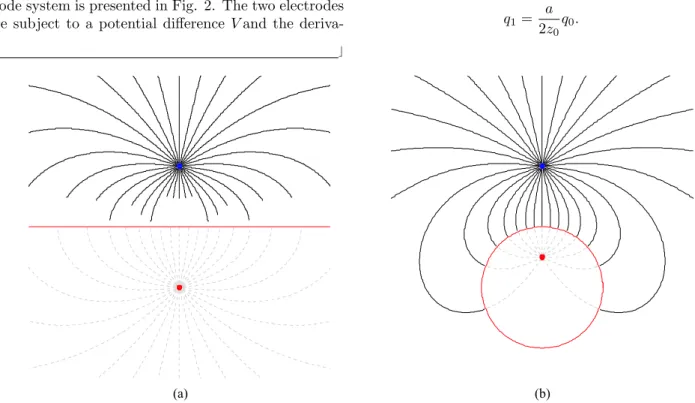
Almost without exception, old and new textbooks on applied electromagnetism discuss the method of images, and this clearly shows the importance of the method for science and engineering. According to Binns, Lawren-son and Trowbridge [7], the essence of the method of images consists in replacing the effects of a boundary related to an applied field by distributions of charges “behind” the boundary line as illustrated in Fig. 1 for two configurations that will be combined to deduce the potential for sphere-plane electrodes. The first config-uration consists of a point charge and a grounded con-ducting infinite plane and this is shown in Fig. 1(a). The second configuration consists of a point charge and a grounded conducting sphere shown in Fig. 1(b). The solid and dashed lines represent the real and virtual fields respectively. The point from where the dashed lines diverge is the image charge. The field pattern, and consequently, the potential distribution for the real electrodes system is equivalent as the one generated by two point charges. The advantage of the image method is that the evaluation of the potential with point charges is simple and straightforward.
A schematic representation of the sphere-plane elec-trode system is presented in Fig. 2. The two elecelec-trodes are subject to a potential difference Vand the
deriva-tion is presented in cylindrical coordinates. According to the chosen reference frame, the conducting plane is placed at the coordinate z= 0 and its electric poten-tial φp is set to zero. The electric potential φs at the spherical electrode is V, being the potential difference between the spherical and the planar electrode. The sphere has radius aand its center is placed atz =z0.
The minimum distance d between the sphere and the grounded plane isd=z0−a.
To find the potential for this system using image charges, we start considering an isolated sphere with charge q0, which generates the potential V at the
sur-face. Then,q0can be expressed in terms of its resulting
potentialV as
q0=
aV
k , (1)
wherek= 9×10⁹Vm/C is the electrostatic constant.
In the presence of the plane atz = 0, chargeq0
gener-ates an image of same magnitude and opposite sign –q0
at position -z0. The image charge –q0also generates an
image in the sphere with position and magnitude given by
z1=z0− a 2
2z0
, (2)
q1=
a
2z0q0. (3)
⌋
(a) (b)
d
r z
a
fp= 0
fs=V
z0
d
r z
a
fp= 0
fs=V
z0
Figure 2 - Schematic representation of the sphere-plane electrodes in cylindrical coordinate system.
This situation is depicted in Fig. 3(a). The image chargeq1, in turn, generates -q1at the plane, which
gen-erates q2 in the sphere and so on. Fig. 3(b) represents
the final charge distribution. The position and magni-tude of the ithimage charge are given by the recurrent relations
zi=z0−
a2
z0+zi−1
, (4)
qi=
a z0+zi−1
qi−1. (5)
The derivation of Eqs. (2) to (5), which can be found in many textbooks, will not be repeated here.
It is convenient to define a normalized charge ξi = qi/q0, that will be used later. Dividing Eq. (5)
byq0 we get
ξi=
a z0+zi−1
ξi−1, (6)
withξ0= 1.
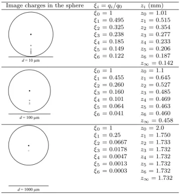
Charge distributions for three configurations of the problem are shown in Table 1. The results show the ef-fect of the minimum distance dbetween the electrodes on the charge distribution in the spherical domain. The first six values of zi and ξi for each d are also pre-sented. It can be noticed from this table that ξi → 0 and zi → z∞ (constant) as i → ∞. In these pictures
the relative magnitude of the charges is represented in a gray scale from black, forξ0(unity), to white, forξ∞
(zero). In fact, these charges have images beneath the plane boundary, but they are not shown for the sake of simplicity. The position and magnitude of these image points are -zi and -qi. The potential for the sphere-plane is equivalent of the potential of these two groups of charges{qi, −qi}.
Table 1 - Schematic illustrations for the image charges and their first 6 values ofξiandzifor 3 distances anda= 1 mm.
Image charges in the sphere ξi=qi/q0 zi(mm)
d= 10mm
ξ0= 1 ξ1= 0.495 ξ2= 0.325 ξ3= 0.238 ξ4= 0.185 ξ5= 0.149 ξ6= 0.122
z0 = 1.01 z1 = 0.515 z2 = 0.354 z3 = 0.277 z4 = 0.233 z5 = 0.206 z6 = 0.187 z∞= 0.142
d= 100mm
ξ0= 1 ξ1= 0.455 ξ2= 0.260 ξ3= 0.160 ξ4= 0.101 ξ5= 0.064 ξ6= 0.041
z0 = 1.1 z1 = 0.645 z2 = 0.527 z3 = 0.485 z4 = 0.469 z5 = 0.463 z6 = 0.460 z∞= 0.458
d= 1000mm
ξ0= 1 ξ1= 0.25 ξ2= 0.0667 ξ3= 0.0178 ξ4= 0.0047 ξ5= 0.0013 ξ6= 0.0003
z0 = 2.0 z1 = 1.750 z2 = 1.733 z3 = 1.732 z4 = 1.732 z5 = 1.732 z6 = 1.732 z∞= 1.732
3.
Solution for the potential, the
elec-tric field and other physical
quanti-ties
The potential due to a charge of indexi in the sphere and its image in the plane is given by
φi =k
Ã
qi
[(z−zi)2+r2]1/2
− qi
[(z+zi)2+r2]1/2
!
. (7)
q0
q1
z =0 z0
-z0 z1
-q0 image ofq0 image of-q0 q0
q1
z =0 z0
-z0 z1
-q0 image ofq0 image of-q0
z =0 z0 -z0 z1 zi z¥ -z1 -zi -z¥ qi -qi z =0
z0 -z0 z1 zi z¥ -z1 -zi -z¥ qi -qi (a) (b)
The potential due to all charges is completely determined by summingφiand using Eqs. (1) and (5) in Eq. (7), results in
φ(r, z) =aV
∞
X
i=0
ξi
[(z−zi)2+r2]1/2
− ξi
[(z+zi)2+r2]1/2
. (8)
It is worth to point out that Eq. (8) is a solution for point charges, which is not the actual system of a sphere-plane. The solution in Eq. (8) is equivalent to the solution of the sphere-plane system only for (z−z0)2+r2 ≥a2
(outside the sphere) and forz ≥0 (above the plane). For the region inside the sphere φ= V at any point and beneath the planeφ= 0 at any point. To account for these regions Eq. (8) has to be redefined as
φ(r, z) =
0 z≤0
V r2+ (z−z
0)2≤a2
aV P∞
i=0
ξi
[(z−zi)2+r2]1/2
− ξi
[(z+zi)2+r2]1/2
otherwise
(9)
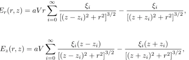
Once φ is given, electric field, capacitance, electrostatic energy and force on the electrodes can be obtained promptly. The electric field can be obtained fromE(r,z) = -∇φand can be written as
Er(r, z) =aV r
∞
X
i=0
ξi
[(z−zi)2+r2]3/2
− ξi
[(z+zi)2+r2]3/2
, (10)
Ez(r, z) =aV
∞
X
i=0
ξi(z−zi) [(z−zi)2+r2]3/2
− ξi(z+zi) [(z+zi)2+r2]3/2
, (11)
whereEr andEz are the components of the field inrand zdirections respectively, so thatE(r, z) =Erˆr+Ezˆz. Fig. 4 shows the potential distribution as a density plot and the electric field lines. Details on the procedure to obtain these figures are shown in Appendix B.
(a) (b)
The sphere-plane electrode system is a capacitor of which the total chargeqis the sum of all charges in the sphere, given by
q=
∞
X
i=0
qi=q0 ∞
X
i=0
ξi. (12)
From the sequences ofξi in Table 1 it can be seen that the largerdis the fasterξi converges. So the num-ber of terms to be summed forqin Eq. (12), to reach a specified accuracy, depends ond. A convergence analy-sis ofq and ofφis presented in the next section.
The capacitance is obtained from C =q/V. Com-bining Eqs. (1) and (12) results in
C= a
k
∞
X
i=0
ξi. (13)
The electrostatic energyU =1/2CV2 is given by
U =aV
2
2k
∞
X
i=0
ξi, (14)
and the force between sphere and planeF = −∂U/∂z0
is
F =−aV
2
2k
∞
X
i=0
ξ′
i. (15)
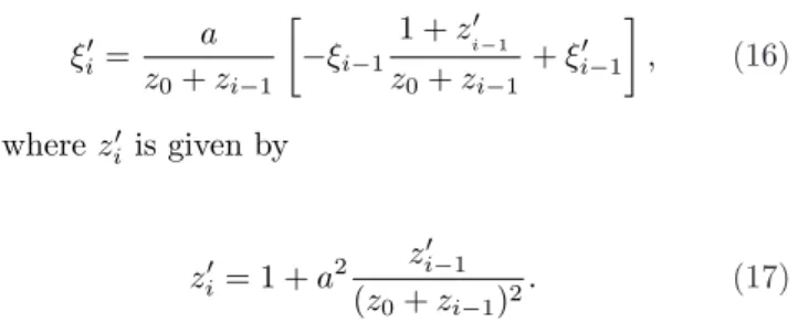
The prime mark indicates a differentiation with re-spect to z0. In this way, differentiation of (6) leads to
the following recurrent relation to computeξ′
i
ξi′=
a z0+zi−1
· −ξi−1
1 +z′ i−1 z0+zi−1
+ξi′−1
¸
, (16)
where z′
i is given by
zi′= 1 +a2
z′
i−1
(z0+zi−1)2
. (17)
The starting conditions for the recurrent relations above areξ′0 = 0 andz0′ = 1. All formulas are
summa-rized in Appendix A. The treatment given above can
also be applied to two spheres. If the spheres have the same size the formulas for the potential distribution are identical to Eq. (8). In this case the symmetry plane of the sphere-sphere problem becomes the plane of the sphere-plane system.
4.
Convergence analysis of charge and
potential
The number of terms needed for the total chargeq in Eq. (12) to converge depends only on the ratio z0/a.
Table 2 shows the number of terms needed forqto con-verge to 99.9 % of its asymptotic value as a function of z0/a.
Table 2 - Number of terms needed for the productk.qto converge as a function ofz0/a.
z0/a k.q(×10−3 Vm) Number of terms to converge to 99.9%
2 1.34 5
1.1 2.15 13
1.01 3.23 34
1.001 4.36 75
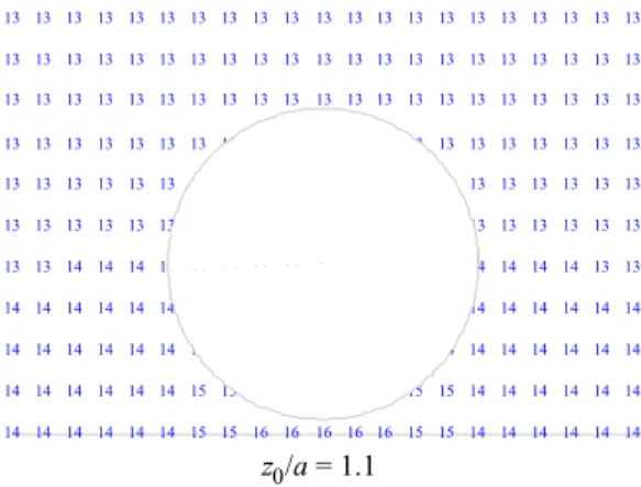
An analysis of the convergence ofφmay be impor-tant as, for example, in fitting processes, where fitting parameters must be varied, then evaluated, and com-pared to experimental results repeatedly. A fitting pro-cedure may take a lot of time and one must avoid com-puting unnecessary terms ofφ. This analysis aims to give a good insight about the convergence behavior, i.e. where the convergence is faster/lower, how the conver-gence varies with z0/a. In Fig. 5 we present the
con-vergence behavior for two cases ofz0/a. In this figure
the numbers represent the number of terms needed for φin Eq. (8) to converge to 99.9 % of the asymptotic value at that point of the space. It can be seen that the region under the sphere needs more terms to con-verge. The number of terms needed is, at most, up to 50 even for z0/a as small as 1.01. For much different
cases than the examples used here, like: much higher accuracy, much wider range of the coordinates, ratio z0/amuch closer to unity, etc, requires an analysis for
37 37 38 38 39 40 41 43 45 49 53 49 45 43 41 40 39 38 38 37 37 37 37 37 38 38 39 40 42 43 45 17 45 43 42 40 39 38 38 37 37 37 37 37 37 38 38 38 39 39 40 39 31 39 40 39 39 38 38 38 37 37 37 36 37 37 37 37 37 37 37 36 35 33 35 36 37 37 37 37 37 37 37 36 36 36 36 36 36 36 36 35 34 31 23 31 34 35 36 36 36 36 36 36 36 36 36 36 36 36 36 35 34 33 32 31 32 33 34 35 36 36 36 36 36 36 36 36 36 36 35 35 35 34 34 33 33 33 34 34 35 35 35 36 36 36 36 36 36 36 35 35 35 35 34 34 34 34 34 34 34 35 35 35 35 36 36 36 36 35 35 35 35 35 35 35 34 34 34 34 34 35 35 35 35 35 35 35 36 35 35 35 35 35 35 35 35 35 35 35 35 35 35 35 35 35 35 35 35 35 35 35 35 35 35 35 35 35 35 35 35 35 35 35 35 35 35 35 35 35 35
14 14 14 14 14 14 15 15 16 16 16 16 16 15 15 14 14 14 14 14 14 14 14 14 14 14 14 15 15 15 16 16 16 15 15 15 14 14 14 14 14 14 14 14 14 14 14 14 14 15 15 15 14 15 15 15 14 14 14 14 14 14 14 14 14 14 14 14 14 14 14 14 14 13 14 14 14 14 14 14 14 14 14 14 13 13 14 14 14 14 13 13 13 12 8 12 13 13 13 14 14 14 14 13 13 13 13 13 13 13 13 13 13 13 12 12 12 13 13 13 13 13 13 13 13 13 13 13 13 13 13 13 13 13 13 12 12 12 13 13 13 13 13 13 13 13 13 13 13 13 13 13 13 13 13 13 13 13 13 13 13 13 13 13 13 13 13 13 13 13 13 13 13 13 13 13 13 13 13 13 13 13 13 13 13 13 13 13 13 13 13 13 13 13 13 13 13 13 13 13 13 13 13 13 13 13 13 13 13 13 13 13 13 13 13 13 13 13 13 13 13 13 13 13 13 13 13 13 13 13 13
z0/a= 1.01 z0/a= 1.1
Figure 5 - Numbers indicate how many terms are necessary for the potential to converge to 99.9% of its asymptotic value at that point of the space.
⌈
5.
Conclusion
We developed the solution for the potential, electric field, capacitance, energy and force for electrodes in a sphere-plane configuration using the method of image charges. Our equation, represented in a cylindrical co-ordinate system, can easily and conveniently be applied to systems with plane-sphere geometry. The method-ology for solving this problem may be used in several other problems of electrostatics. We are confident that
our treatment can conveniently be applied by students and engineers working on electrostatics.
Acknowledgments
We greatly acknowledge the help of Dr. Pablo Paredez, Ms. Aline Marque and Dr. Daniel den Engelsen for the help in preparing this manuscript. Authors are grateful to the Brazilian funding agencies CNPq and Fapesp for
financial support. ⌋
Appendix A: Formulary
Image charge position zi=z0− a
2
z0+zi−1fori >0
Initial (central) charge q0=aVk
I
IImage charge magnitude qi= z0+azi
−1qi−1fori >0
I
IRelative charge magnitudeqi/q0 ξi=z0+az
i−1ξi−1fori >0
I
I∂zi/∂z0 z0′ = 1;
I
Iz′
i= 1 +a2 z′
i−1
(z0+zi−1)2 fori >0
∂ξi/∂z0 ξ′0= 0;
I
Iξ′
i= a
z0+zi−1[−ξi−1
1+z′ i−1
z0+zi−1+ξ
′
i−1] fori >0
Total charge q=q0P∞i=0ξi
I
IPotential φ(r, z) =
0 z≤0 II
V r2+ (z−z
0)2≤a2 aVP∞
i=0
ξi [(z−zi)2+
r2
]1/2 −
ξi [(z+zi)2+
r2
]1/2 otherwise
Electric field:rcomponent Er(r, z) =aV rP
∞
i=0
ξiII [(z−zi)2+r2]3/2−
ξi [(z+zi)2+r2]3/2
Electric field:zcomponent Ez(r, z) =aV P∞i=0 ξi(z
−zi)II [(z−zi)2+r2]3/2−
ξi(z+zi) [(z+zi)2+r2]3/2
Capacitance C=a
k P∞
i=0ξi
I
IEnergy U=aV2k2P∞
i=0ξi
I
IForce F =−aV
2
2k P∞
i=0ξ ′
i
I
Appendix B: Algorithms and programs
for rendering graphics
Once the equations for the potential and the electric fields are established their corresponding graphics can be rendered for a visual presentation of the solution. This is not a trivial procedure. Many high level pro-gram languages are available for algebraic manipulation and graphics. In this section we will line out a proce-dure inMathematica°R [8]- a software with a very high
level programming language- that we used to render the figures shown in this article. Next sections will provide an overall procedure to do the programs in Mathemat-ica and will present the programs used.
B1. Image charges in the sphere
The figures shown in Fig. 3 and Table 1 was obtained as follows:
1. Numerical values are attributed toz0,a.
2. Normalized charges ξi and their positions zi are calculated fori from 0 to 100, which is more than suf-ficient.
3. The representation of the sphere, the plane and the points (0,zi) are drawn using built-in com-mands Circle[...], Line[...] and Point[...] respectively. The points are rendered in gray level using command GrayLevel[...].
4. Graphics are merged and rendered.
The program used is shown below. An animation can be found in the internet with URL given in Ref. [9].⌋
Clear[i,a,z,zi,r,z0]; "Clear parameters attributions"; a=10^-3; "radius of the sphere";
d=10^-5; "distance sphere-plane";
z0=a+d; "z coordinate of the sphere center"; nter=100; "number of image charges to compute"; zi[0]=z0; "position of first charge";
xsi[0]=1; "magnitude of first charge";
Do[
zi[i]=z0-a^2/(z0+zi[i-1]); "z positions of image charges";
xsi[i]=a xsi[i-1]/(z0+zi[i]); "normalized magnitude of image charges"; ,{i,nter}];
ImageCharges= Table[{PointSize[0.02], GrayLevel[1-xsi[i]], Point[{0,zi[i]}]}, {i,nter,0,-1}]; "Image charges characteristics to be drawn as points";
G=Graphics[{Circle[{0,z0},a], Line[{{-a,0},{a,0}}], ImageCharges}, AspectRatio-> 1, PlotRange->All]; "Draw of the circle and the line and the points";
Show[G, AspectRatio->(z0+a)/(2a)];
"Render the circle, the line and the points in the same graphic";
B2. Density plot of the potential
To render Fig. 4(a):
1. We attributed numbers to parametersaandz0.
2. We computedzi andξi forifrom 0 to 100.
3. We wrote the potential as in Eq. (9) likeφ= If[condition,then,else], whereconditionis (z−z0)2+r2≥a2,
block then must be the expression forφoutside the sphere and blockelse is the expression forφinside the sphere
(V).
4. We rendered the potential with built-in command DensityPlot[φ(r,z)]. The program used is shown below. See also URL in Ref. [10].
Clear[i,a,d,z0,nter,zi,xsi,Fi]; "Clear all variables that will be used";
a=0.001; "radius of the sphere"; d=0.0001; "distance sphere-plane";
z0=a+d; "z coordinate of the center of the sphere";
V=1; "potential at the sphere";
zi[0]=z0; "position of the i(th) image charge";
xsi[0]=1; "relative magnitude of the i(th) image charge";
Do[
zi[i]=z0-a^2/(z0+zi[i-1]); "z position of the image charges";
xsi[i]=a xsi[i-1]/(z0+zi[i-1]); "normalized magnitude of the image charges"; ,{i,nter}];
Fi=If[(z-z0)^2+r^2>=a^2,
a V Sum[xsi[i]/Sqrt[(z-zi[i])^2+r^2]-xsi[i]/Sqrt[(z+zi[i])^2+r^2], {i,0,nter}], V]; "Attribution of a function to the potential outside and inside the sphere.";
DensityPlot[Fi, {r,-2a,2a}, {z,0,4a}, Mesh-> False, Frame-> False, PlotPoints-> 200, AspectRatio-> 1];
"Render the potential as a Density plot.";
B3. Field lines between the electrodes
To render Fig. 4(b):
1. We attributed numerical values toa,z0 and few other parameters used.
2. We computedzi andξiforifrom 0 to 100.
3. We attributed expressions for the electric field functions ErandEz as in Eqs. (10) and (11).
4. Points on the circle that represents the sphere where selected as starting points of the electric field line. The starting point of each electric field line is not equally spaced from each other. Their spacing is proportional to the strength of the electric field, relative to the maximum field at the bottom of the sphere. This is done so the reader can visualize the field strength by the density of the field lines.
5. The field line is built, point by point, using the coordinate of the previous point plus a constant step toward the field direction to calculate the next point of the field line. New points are calculated until the field line reaches the border of the region to be shown in the graphic. The points are stored in a list and plotted.
The program is shown below. See also Ref. [11]. Fig. 1(a) and (b) are particular cases of this program and will not be shown here. Animations of Fig. 1(a) can be seen in Ref. [12].
"Clear parameters";
Clear[a,d,z0,V,nter,zi,xsi,nlines,del,i,ii,j,k,r,z,rfl,zfl,fieldline,Er,Ez,Emod,tet,pretet]; a=0.001;"Sphere radius";
d=0.0001;"distance sphere-plane";
z0=a+d;"z coordinate of the center of the sphere"; V=1;"Voltage at the sphere";
zi[0]=z0;"z positions of the initial charge";
xsi[0]=1;"normalized magnitude of the initial charge"; nter=100;"number of terms to compute the electric field"; nlines=50;"number of field lines to draw";
del=a/100.;"step distance between two points in a field line";
Do[fieldline[j]={},{j,nlines}];"list to store the points of the k(th) field line "; Do[
zi[i]=z0-a^2/(z0+zi[i-1]);"z positions of the image charges"; xsi[i]=a xsi[i-1]/ (z0+zi[i-1]);
"normalized magnitude of the image charges"; ,{i,nter}];
Er=a V r Sum[xsi[i]/((z-zi[i])^2+r^2)^(3/2)-xsi[i]/((z+zi[i])^2+r^2)^(3/2),{i,0,nter}]; "r component of the electric field";
"z component of the electric field";
Emod=Sqrt[Er^2+Ez^2]; "module of the electric field"; Do[
pretet=Abs[1/Emod]/.{r->a Sin[2 Pi k/nlines],z->z0-a Cos[2 Pi k/nlines]};
"pretet is auxiliary to determine the points on the sphere at which a field line will depart"; tet=2Pi Sum[pretet,{k,j}]/Sum[pretet,{k,nlines}];
"tet is the angle between z-axes and the point at the sphere at which a field line will depart"; rfl[0]=a Sin[tet];"initial r coordinate of the j(th) field line";
zfl[0]=z0-a Cos[tet];"initial z coordinate of the j(th) field line";
"---Block to build the j(th) field line---"; ii=0;"couter";
While[rfl[ii]\[GreaterEqual]-2a && rfl[ii]<=2a && zfl[ii]>=0 && zfl[ii]<=4a, ii++;"Increment ii";
rfl[ii]=(r+Er/Emod del)/.{r->rfl[ii-1],z->zfl[ii-1]}; "r coordinate of the ii(th) point of the j(th) field line"; zfl[ii]=(z+Ez/Emod del)/.{r->rfl[ii-1],z->zfl[ii-1]}; "z coordinate of the ii(th) point of the j(th) field line"; AppendTo[fieldline[j],{rfl[ii],zfl[ii]}];
"Append last calculated point (rfl,zfl) to the j(th) field line"; ];
"---"; P[j]=ListPlot[fieldline[j],PlotJoined->True,PlotRange->{{-2a,2a},{0,4a}},
DisplayFunction->Identity];
,{j,nlines}];"Store the graphics of the j(th) field line in P[j]"; Plist=Table[P[j],{j,nlines}];"Does a list with all field lines"; G=Graphics[{RGBColor[1,0,0], Circle[{0,z0},a]}];
"Store in G the graphics of the field lines and the sphere";
Show[{Plist,G},Ticks->None,Axes->{True,False},AspectRatio->1, DisplayFunction-> $DisplayFunction]; "Render the field lines and the sphere together";
"---";
⌈
References
[1] W.R. Smythe, Static and Dynamic Electricity (McGraw-Hill, New York, 1950), 2nd ed.
[2] J.C. Maxwell,A Treatise in Electricity and Magnetism (Dover, New York, 1958), v. 1 3rd ed.
[3] O.J. Lodge, Proc. Phys. Soc. London.2,24 (1875).
[4] A. Foster, Theoretical Modeling of Non-contact Atomic Force Microscopy on Insulators. PhD The-sis, University College London, 2000. Available at
[5] D.A. Lowther and E.M. Freeman, IEEE Trans. Educ. 36, 219 (1993).
[6] J.H. Cloete and J. van der Merwe, IEEE Trans. Educ. 41, 141 (1998).
[7] K.J. Binns, P.J. Lawrenson and C.W. Trowbridge,The Analytical and Numerical Solution of Electric and Mag-netic Fields(John Wiley & Sons, Chichester, 1992), p. 93.
[8] Available at
[9] Available at
See also
[10] Available at
[11] Available at
[12] Available at