Electrostatics of two suspended spheres
(Eletrost´atica de duas esferas suspensas)
Fernando Fuzinatto Dall’Agnol
1, Victor P. Mammana and Daniel den Engelsen
Centro de Tecnologia da Informa¸c˜ao Renato Archer, Campinas, SP, Brasil Recebido em 25/2/2011; Aceito em 6/2/2012; Publicado em 21/11/2012
Although the working principle of a traditional electroscope with thin metal deflection foils is simple, one needs numerical methods to calculate its foil’s deflection. If the electroscope is made of hanging spheres instead of foils, then it is possible to obtain an analytical solution. Since the separation of the charged spheres is of the order of their radius the spheres cannot be described as point charges. We apply the method of image charges to find the electrostatic force between the spheres and then we relate the voltage applied to their separation. We also discuss the similarity with the sphere-plane electrostatic problem. This approach can be used as an analytical solution for practical problems in the field of electrodynamics and its complexity is compatible with undergraduate courses.
Keywords: electroscope, electrometer, method of image, image charge, electrostatic, sphere-sphere.
Apesar da simplicidade do princ´ıpio de funcionamento do eletrosc´opio tradicional feito de folhas met´alicas finas, ´e necess´ario m´etodos num´ericos para calcular a deflex˜ao das folhas. Se o eletrosc´opio for feito de esferas penduradas ao inv´es de folhas, ent˜ao ´e poss´ıvel obter uma solu¸c˜ao anal´ıtica. Como a deflex˜ao das esferas car-regadas ´e da ordem dos seus raios, as esferas n˜ao podem ser descritas como cargas pontuais. N´os aplicamos o m´etodo das cargas imagens para encontrar a for¸ca eletrost´atica entre as esferas, e ent˜ao, correlacionamos a voltagem aplicada com a separa¸c˜ao. Discutimos tamb´em as similaridades com o problema eletrost´atico de uma esfera e um plano. Esta abordagem pode ser usada como uma solu¸c˜ao anal´ıtica para problemas pr´aticos em eletrodinˆamica e sua complexidade e compat´ıvel com cursos de gradua¸c˜ao.
Palavras-chave: eletrosc´opio, eletrˆometro, m´etodo das imagens, carga imagem, eletrost´atica, esfera-esfera.
1. Introduction
The electroscope is an instrument presented to students in their introduction to electrostatics as a demonstra-tion of the existence of electric charges (Fig. 1). His-torically, this instrument was also important in the de-velopment of electricity [1]. If the electroscope is cali-brated to provide the value of the charge (or the volt-age) it is often called an electrometer. Usually, electro-scopes are made of very light deflectable metal foils, in which it is impossible to calculate the charge they can store analytically. We describe here the properties of two suspended and electrically connected spheres that can move in a vertical plane only: in this case an an-alytical solution of the separation of the spheres can be found. We shall use themethod of images to corre-late the applied voltage to the deflection of the spheres. Applying this method is easier than solving Laplace’s equation directly [2].
In the introduction courses to electrostatics, many exercises involve charged spheres. Usually the problem
is simplified by regarding the spheres as point charges. We shall show that the error in the determination of the force between the spheres or any other physical quan-tity (applied voltage; total charge, etc) can be large, if the image charges are ignored. Moreover, in real appli-cations the point charge approximation for spheres can usually not be applied. For example, in those funny hair bristle Van de Graaff generators for educational purposes (Fig. 2), the main sphere and the spherical accessories used in the apparatus are manipulated at small distances, so the effect of image charges is quite large. In these cases to evaluate the total charge, the voltage, or the force, etc, it is important to take these image charges into account.
2.
Method of image charge
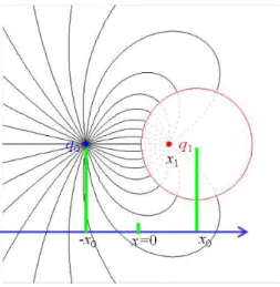
Figure 3 illustrates the method of image charge for a point charge close to a grounded sphere [3,4]. Consider the sphere with radiusa centered at x0 and the point
charge,q0, placed at -x0. The solution for the electric
1E-mail: [email protected].
potential can be determined as if an image charge q1
was at positionx1. The point chargeq1 is virtual; the
real charge induced is actually distributed at the sur-face of the sphere. The solid and dashed lines represent the real and virtual field lines respectively. Click the URL in Ref. [5] to watch an animation of the electric field lines as a function ofx0. The potentialφmust be
identically zero everywhere at the surface of the sphere particularly
Figure 1 - The Electroscope of leaves; the deflection of the foils is impossible to be calculated analytically.
Figure 2 - Van de Graaff generator showing the main sphere and an accessory sphere at small distance compared to their diame-ters. This is usually the case in real electrostatic systems and the image charges must be taken into account.
Figure 3 - Illustration of the method of images: a real chargeq0
induces an opposite chargeq1 in a grounded sphere. The charge
induced is as ifq1be a point charge located atx1.
φ(x0−a) =k
( q
0
2x0−a+
q1
x1−(x0−a)
)
= 0, (1)
φ(x0+a) =k
(
q0
2x0+a
+ q1
x0+a−x1
)
= 0, (2)
wherekis dielectric constant of vacuum. Alsoφ(∞) = 0 by definition. Solving the system above we have
q1=− a 2x0
q0, (3)
x1=x0− a
2
2x0
. (4)
3.
Electroscope with two spheres
Assume an electroscope made of two identical con-ductive spheres. The spheres have radius a, mass m
and they hang from two massless conductive wires; so, the spheres are electrically connected. The wires have length L and separation 2a. The capacitance of the wires is negligible so only the spheres store charge. When the electroscope is neutral (Fig. 4a) the spheres touch each other, but with no contact force. In this situation, we assume the voltageφ= 0 at the spheres. If a voltage φ = V is applied (Fig. 4b), the spheres becomes separated byd. In this problemdis the mea-surable variable so the problem is to findV as a function of the separationd.
In calculating the electric potential one must define its value at some point in the space in the physical sys-tem. Usually it is convenient to makeφ= 0 at infinity as is the case here, so when the spheres are uncharged
φ must equal zero also at the spheres. Then, there is no electric field because there is no potential difference in the system.
4.
Solution for the electric force
A simplification of the electroscope is depicted in Fig. 5, in which only the spheres are shown. The sphere-sphere problem is very similar to the sphere-plane problem that we described in detail in Ref. [6]. Any difference between these two solutions will be discussed.
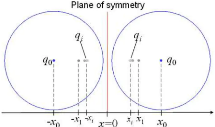
Figure 5 - When two spheres of chargeq0are approximated each
one generates a series of image charges{qi}into the other.
Starting from central charges q0, each of these
in-duces q1 at the other sphere, which in turn induces
back a charge q2 and so on. The distribution of the
total charge,q, is equivalent to a series of point charges
qi. The solution is symmetric with respect to the plane
x= 0.
Applying the procedure of section 2 the positions and the magnitude of the image charges are given by the recurrent relations
xi>0=x0− a
2
x0+xi−1
(5)
and
qi=
−a
x0+xi−1
qi−1, (6)
where
x0=d/2 +a (7)
and
q0=
aV
k . (8)
It is convenient to define a dimensionless relative charge, ξi, as the ratio between the ith image charge
and the central charge q0
ξi>0= qi
q0
= −a
x0+xi−1
ξi−1, (9)
withξ0= 1. The negative sign in Eqs. (6) and (9) does
not appear in the sphere-plane problem, because there the electrodes have opposite charges. Here, the image charges in the spheres have alternating signs, while the
image charges in the sphere-plane problem are all pos-itive in the sphere and all negative in the plane. The total charge in each sphere is given by
q=
∞
∑
i=0
qi=q0 ∞
∑
i=0
ξi. (10)
Let the parameter ξ, with no index be the total charge compared to the central charge as
ξ=
∞
∑
i=0
ξi. (11)
Now that xi and ξi are determined, the derivation
of the force,F, between the spheres is straightforward. The force between a point charge with index i in one sphere and a point charge with index j in the other sphere is given by Coulomb’s law
Fij =kq20
ξiξj
(xi+xj)2
. (12)
Replacingq0for the expression in Eq. (8) the total
force is the summation over all pairs (i,j)
F =(aV)
2
k
∞
∑
i=0 ∞
∑
j=0
ξiξj
(xi+xj)2
. (13)
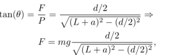
Figure 6 shows the deflection of one sphere’s cen-ter when the electroscope is charged. The equilibrium among the electrical force, the weight (P) and the ten-sion in the wire correlatesV anddaccording to
tan(θ) =F
P =
d/2
√
(L+a)2−(d/2)2 ⇒
F=mg√ d/2
(L+a)2−(d/2)2
, (14)
where g is the acceleration of gravity. By combining Eqs. (13) and (14) we get an expression forV
V =
v u u u t
kmg
a2 ∞
∑
i=0 ∞
∑
j=0 ξiξj (xi+xj)2
d/2
√
(L+a)2−(d/2)2
. (15)
5.
Convergence analysis
Table 1 shows the values forxiandξifora= 1 arbitrary
length unit (a.u). andd= 0.1 a.u. The image charges positions tend fast tox∞=
√
x2
0−a2 and the relative
charges magnitudes tend toξ∞ = 0. The greater isd,
the faster is the convergence [6].
Table 1 - Relative charge magnitude and their positions for
d/a= 0.1.
ξ0 = 1
ξ1=−0.47619
ξ2 = 0.29326
ξ3=−0.19759
ξ4 = 0.13854
ξ5=−0.09904
ξ6 = 0.07150
ξ∞= 0
x0 = 1.05
x1 = 0.57381
x2 = 0.43416
x3 = 0.37622
x4 = 0.34885
x5 = 0.33513
x6 = 0.32804
x∞= 0.320156
Figure 7 shows V for several values of d in a.u.,
a = 1 a.u., L=10 a.u. and m = 10−4
kg. The
right axis of Fig. 7 shows the normalized total charge
ξ. Even for d as large as 5 times the radius of the spheres,ξis yet 87%,i.e. the total charge is only 87% of the central charge. This means that the comple-mentary 13% is typically the error one would have in
F by ignoring the image charges in the spheres. It can be seen in Fig. 7 that the voltages to deflect the spheres are quite high. However, rubbed objects can easily obtain voltages greater than 100 kV. Such high voltages may cause a sudden discharge of the electro-scope, since the dielectric break down limit in air is
Emax ∼= 3 MV/m; so, arcing will occur if an external
object is brought close to the spheres, say at a dis-tance < 1 mm [7]. An upper limit of the measurable voltage can be estimated from the field of one of the spheres: Emax = Vmax/a ⇒ Vmax = 30 kV. This
value is overestimated by∼10% according to the error discussed above. Anyway, it gives a good estimative for the maximum measurable voltage. For a = 1 cm, one gets maximum measurable separation of dmax ∼=
4.5 cm. Figure 8 illustrates the norm of the electric
field nearby the spheres for d = 0.5a. This figure was made using the expressions for the electric field pre-sented in the appendix. The electric field is maximum at the outer poles of the spheres in the blue regions.
Figure 7 - Curves for the voltageV (solid line) and for the relative chargeξ(dashed curve).
Figure 8 - Density plot of the electric field distribution for
d= 0.5a. The shades of blue indicate strong electric field re-gions.
6.
Conclusion
We obtained an analytical solution for an electroscope of two suspended spheres using the method of image charges. This is a simple and representative solution: it can easily be generalized to more spheres, spheres of different sizes and dielectric spheres. Not taking the in-duced image charges into account in this problem will lead to a significant error in the evaluation of the total charge and voltage. Our calculation also indicates that an electroscope with two metal spheres needs rather high voltages to get deflection; however, those high voltages needed are easily obtained by rubbing objects. The maximum deflection is obtained when the electric field strength close to the spheres reaches the dielectric breakdown limit in air.
Appendix: formulary
Image charge positions xi>0=x0− a 2 x0+xi−1
Initial (central) charge q0=aVk
Image charge magnitude qi=
−a x0+xi−1
qi−1
Relative charge magnitudeqi/q0 ξi>0=qq0i = −a
x0+xi−1 ξi−1
Total charge q=q0
∞ ∑
i=0
ξi
Potential (valid outside the spheres) φ(r, x) =aV
∞ ∑
i=0
ξi
[(x−xi)2+r2]
1/2
+ ξi
[(x+xi)2+r2]
1/2
Electric field: rcomponent (valid outside the spheres) Er(r, x) =aV r
∞ ∑
i=0
ξi
[(x−xi)2+r2]
3/2
+ ξi
[(x+xi)2+r2]
3/2
Electric field: xcomponent (valid outside the spheres) Ex(r, x) =aV
∞ ∑
i=0
ξi(x−xi)
[(x−xi)2+r2]
3/2 +
ξi(x+xi)
[(x+xi)2+r2]
3/2
Capacitance C=2a
k
∞ ∑
i=0
ξi
Force F= (aV)
2
k
∞ ∑
i=0 ∞ ∑
j=0
ξiξj
(xi+xj)2
7.
Acknowledgments
The authors are grateful to the Brazilian funding agen-cies CNPq and Fapesp for financial support.
References
[1] A. Medeiros, Revista Brasileira de Ensino de F´ısica24, 353 (2002).
[2] J.D. Love, Quarterly J. Mechanics Appl. Math.28, 449 (1975).
[3] W. R. Smythe, “Static and Dynamic Electricity”, 2nd ed. New York: McGraw-Hill, (1950).
[4] J.D. Jackson, Classical Electrodynamics (Wiley, New York, 1975), 3rd ed.
[5] http://www.youtube.com/watch?v=HmZjHGG_4cQ.
[6] F.F. Dall’Agnol and V.P. Mammana, Revista Brasileira de Ensino de F´ısica31, 3503 (2009).