The Term Structure of Interest Rates and its Impact on the Liability
Adequacy Test for Insurance Companies in Brazil
Antonio Aurelio Duarte
Fundação Escola de Comércio Álvares Penteado, Programa de Mestrado em Ciências Contábeis, São Paulo, SP, Brazil
Aldy Fernandes da Silva
Fundação Escola de Comércio Álvares Penteado, Programa de Mestrado em Ciências Contábeis, São Paulo, SP, Brazil
Luciano Vereda Oliveira
Universidade Federal Fluminense, Departamento de Economia, Niterói, RJ, Brazil
Elionor Farah Jreige Weffort
Fundação Escola de Comércio Álvares Penteado, Programa de Mestrado em Ciências Contábeis, São Paulo, SP, Brazil
Betty Lilian Chan
Fundação Escola de Comércio Álvares Penteado, Departamento de Ciências Contábeis, São Paulo, SP, Brazil
Received on 04.09. 2014 – Desk acceptance on 04.13.2014 – 3th version approved on 01.09.2015.
ABSTRACT
The Brazilian regulation for applying the Liability Adequacy Test (LAT) to technical provisions in insurance companies requires that the current estimate is discounted by a term structure of interest rates (hereafter TSIR). This article aims to analyze the LAT results, derived from the use of various models to build the TSIR: the cubic spline interpolation technique, Svensson’s model (adopted by the regulator) and Vasicek’s model. In order to achieve the objective proposed, the exchange rates of BM&FBOVESPA trading days were used to model the ETTJ and, consequently, to discount the cash flow of the insurance company. The results indicate that: (i) LAT is sensitive to the choice of the model used to build the TSIR; (ii) this sensitivity increases with cash flow longevity; (iii) the adoption of an ultimate forward rate (UFR) for the Brazilian insurance market should be evaluated by the regulator, in order to stabilize the trajectory of the yield curve at longer maturities. The technical provision is among the main solvency items of insurance companies and the LAT result is a significant indicator of the quality of this provision, as this evaluates its sufficiency or insufficiency. Thus, this article bridges a gap in the Brazilian actuarial literature, introducing the main methodologies available for modeling the yield curve and a practical application to analyze the impact of its choice on LAT.
1 INTRODUCTION
to 12.35% of GDP, and they reached annual revenue (insu-rance, pension, and capitalization) of R$ 156.9 billion (Supe-rintendência de Seguros Privados, 2013). he strong market expansion, in terms of annual revenues and representativeness in relation to GDP can be viewed in Figure 1.
In 2012, despite a contraction in the national gross do-mestic product (GDP), expansion indicators of the insurance market exceeded all expectations. Insurance companies have demonstrated a strong ability of domestic savings generation, reaching R$ 543.7 billion in investments, which corresponds
Due to its economic representativeness and the so-cial and political implications of this activity, in Brazil, insurance companies are subject to specific regulation and surveillance by the Superintendence of Private In-surance (SUSEP).
Law 11,638, enacted on 28 December 2007, provi-des that regulatory bodies and agencies can adopt the statements issued by entities whose object is the study and dissemination of accounting principles, standar-ds, and patterns. Thus, SUSEP issued the Circular 408, in August 2010, establishing that insurance companies comply with the International Financial Reporting Stan-dards (IFRS) when preparing and presenting their con-solidated financial statements, adopting the internatio-nal accounting standard, as approved by the Accounting Statements Committee (CPC).
An aspect relevant to the field of activity under analy-sis in this article is the Technical Statement CPC 11 – In-surance Contracts – and the statement derived from the IFRS 4 – Insurance Contracts –, whose aim is specifying
the accounting recognition for insurance contracts. Ac-cording to Bostan (2011, p. 132), “the introduction of the IFRS 4 produces, therefore, a strong impact not only over the accounting, but also over the management of the assets in the balance sheet of the insurance compa-nies.” When referring to the adoption of the IFRS in the European Union (January 1, 2005), Agliata, Maglio, Fer-ron, and Tuccillo (2011, p. 6) observe that, by adopting the IFRS 4, the regulator shows the intention to “regula-te in unison the evaluation of the ‘insurance liabilities’, in consistency with the conceptual assumptions of an accounting model inspired by the ‘Asset and Liability’ view.”
The Technical Statement CPC 11 also establishes the LAT, i.e. Liability Adequacy Test. In order to regulate this test, SUSEP issued the Circular 410/2010 (later on repealed by the Circular 457/2012), which established the LAT for purposes of financial statements and defines rules and procedures for its use.
Lindberg and Seifert (2010, p. 235) explain that
[…] at each reporting date, the insurer must assess whether its recognized insurance liabilities are adequate, using cur-rent estimates of future cash flows under any outstanding insurance contracts. This is known as a “liability adequacy test.” The test should consider the current estimates of all contractual cash flows, including the costs of handling clai-ms and any embedded options and guarantees.
The LAT aims to verify whether the technical pro-visions constituted by insurance companies, deducted from deferred acquisition expenses and related intan-gible assets (net carrying amount) are sufficient to su-pport the net current value of future cash flows of its insurance contracts, discounted by a term structure of interest rates (TSIR) – current estimate. Thus, the LAT consists in calculating the difference between the cur-rent estimate and the net carrying amount. If the di-fference is positive, an inadequate provisioning of the insurance company is characterized, which should be recognized immediately.
he LAT was born within the IFRS, whose main fea-ture is being based on principles. he freewill intrinsic to this accounting requires, on the other hand, the respon-sibility to properly justify the criteria adopted to ground one’s own choices. hus, standardizing the yield curves, or any other parameter, and make them available to all agents contradicts an accounting based on principles.
The countries that joined the IFRS provided their regulators with freedom to keep local rules on indivi-dual publications. Thus, the same company should com-ply with the international standards for consolidated publication according to the IFRS standards and, also, with local rules for individual publication according to the standards of its regulator. Regarding the TSIR, most countries kept their discretion.
According to Post, Gründl, Schmidl, and Dorfman (2007, p. 251),
[…] whether the volatility of the financial position of an insurance company will also increase depends on the ac-counting system adopted until migration to the IFRS. If the insurance company has come from a very conservati-ve accounting regime (e.g. French or German GAAP) to the IFRS, then the volatility of equity will certainly increa-se. In contrast to the pre-IFRS accounting, both assets and liabilities become sensitive to current price fluctuations in the capital market and stock variations in costs associated with the exercise of rights by customers.
In Brazil, SUSEP defines the yield curve to be used in the LAT. Anyway, although Brazilian insurance com-panies use the TSIR provided by SUSEP for individual publication, they should choose and justify that choice, as well as the model for generation of the yield curve that will be used in the publication of their consolidated financial statements according to the IFRS patterns.
In this regulatory context, the TSIR starts playing a key role in the discussion of the LAT, as it is one of the
most sensitive components in the test methodology. Ac-cording to Franklin Jr., Duarte, Neves, and Melo (2011, p. 2): “One of the most relevant elements for calculating the liability adequacy test is the estimation of the term structure of interest rate (TSIR), obtained from financial instruments regarded as free from credit risk available in the Brazilian market.” In addition to the test elasticity in relation to the interest rate, it is faced with a choice dilemma, due to the fact the literature offers a range of possible methodologies for extrapolation and interpola-tion of interest rates, all of them technically grounded and widely adopted by the financial market.
The TSIR represents the discount rate used to mea-sure the value of money over time. It is subject to fluc-tuations, due to the forces of asset supply and demand, i.e. the market is among the components involved in the formation of the yield curve. The Market Segmentation Theory, initially proposed by Culbertson (1957), provi-des this fact with a basis by demonstrating that agents have very definite preferences about the time over which they intend to invest or raise funds, and the supply and demand forces concerning the bonds maturing within this region will define the interest rates, indeed, which, in turn, will form the TSIR.
Technical provisions, in turn, do not have this featu-re (Mano & Ferfeatu-reira, 2009). Although the methodolo-gy to calculate the provisions is in line with the concept of current estimate, by assessing liabilities, through the projection of future cash flow of insurance contracts, its flow is discounted by contractual interest rates or rates that meet a prudential view assuming the use of a cer-tain degree of caution to set the parameters, in order to preserve the solvency capacity, which do not fluctuate according to the bond market. There is also a need to observe that the interest rates used when “pricing” an insurance contract are not compatible with the interest rates used in pricing fixed income bonds, among other reasons, because while the first contract is not negotia-ble (hindering its evaluation in terms of market value), the second enjoys a liquid and regulated market.
hus, by submitting these provisions to the LAT, we are faced with a conlicting situation where the deicit of a period may follow the surplus of the next period, without changing the risk of an insurance with which these provi-sions were designed to support. In this hypothetical case, reversal of the results of the LAT might be explained solely by the natural oscillation of the TSIR. he European regu-lator, i.e. the European Insurance and Occupational Pen-sions Authority(EIOPA), makes clear its position on this matter: “he assessment of technical provisions and the solvency position of an insurance or re-insurance company should not be unduly distorted by strong luctuations in the short-term interest rates” (Committee of European Insu-rance and Occupational Pensions Supervisors, 2010, p. 4).
answer the following question: “Can the choice of the TSIR methodology inluence on the conclusion of suiciency or insuiciency of provision for the purposes of the LAT?”
The general objective of this article is analyzing the LAT results derived from the use of the cubic spline inter-polation technique, Svensson’s parametric model (whi-ch was adopted by the regulatory body) and Vasicek’s one-factor equilibrium model to build the TSIR, which will be used to discount the predicted cash flow (current estimate) of liabilities derived from insurance contracts with a survival coverage.
This research is justified because the current gap be-tween the prudential view of the calculation of provi-sions and the fair value view of the adequacy test has in-creased, due to the fact that the TSIR is one of the most sensitive test components. This leads the methodology adopted to build the yield curve acquires great impor-tance regarding the LAT results, as the degree of insu-fficiency or suinsu-fficiency of provision will depend on the model choice to build the TSIR. However, another TSIR model, also legitimate, might be chosen and, as a conse-quence, another LAT result could be obtained. Reversal provisions, in the case of test surplus, and the formation
of provisions where the deficit takes place, impact on the company’s bottom line and interfere with the distribu-tion of dividends and the payment of taxes. They are also mentioned in the notes and compromise the solvency analysis conducted by the insurance company.
he technical provision is among the main solvency items of insurance companies and the LAT result consti-tutes a signiicant indicator of the quality of this provision, as it evaluates the suiciency or insuiciency of provisio-ning. Due to this fact, insurance companies need to show a good performance in the suitability tests. As the LAT methodology is sensitive to the TSIR chosen, insurance companies have a marked interest in knowing the models available to build it and the impact these choices have on their adequacy tests. hus, this article bridges a gap in the Brazilian actuarial literature, by introducing the main me-thodologies available for modeling the yield curve.
his article is organized this way: introduction of the theoretical framework of the main elements making up the LAT (section 2); description of the methodological proce-dures, including the database and the parameters set for the models (section 3); discussion of the main results of tests and analyses (section 4); and inal remarks (section 5).
2 THEORETICAL FRAMEWORK
In this section, we introduce the theoretical fra-mework of the main elements making up the LAT: the technical provisions and the TSIR.
2.1 Technical provisions.
An insurance company is intended to provide gua-rantees for future risks, uncertain and potential, which may cause financial losses to its policyholders and par-ticipants. On the other hand, they receive, from the lat-ter ones, premiums or contributions fit to the respective guarantees. By accepting these risks, insurance compa-nies take future financial commitments that, in certain situations, can exceed, many times over, their fiscal year revenue. For keeping solvency, insurance companies form technical provisions, which are financial reserves
sized to meet the needs of future financial commitments arising from the risks taken. In Brazil, the technical pro-visions, constituted by insurance companies, are delimi-ted by the National Council of Private Insurance (CNSP) and regulated by SUSEP, by means of its circulars. Accor-ding to Decree 66,408/1970, the actuary is the professio-nal responsible for calculating the technical provisions.
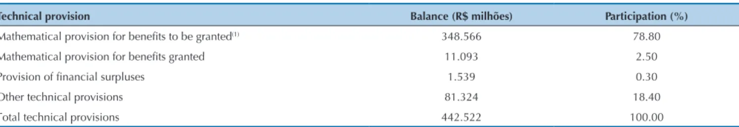
This article outlines the study to the current estima-te of future cash flows relaestima-ted to the survival guaranestima-tee operations (pension plans) offered by insurance compa-nies. This business segment was chosen due to the fact it encompasses long-term contracts, where the effects of the TSIR are more noticed. Table 1 shows the majority stake over 80% of these reserves in the total provisioning of insurance companies for December 2013.
Source: SUSEP (2012).
(1) Includes hedge-fund capitalization.
Table 1 Technical provisioning made by the insurance market in December 2013
Technical provision Balance (R$ milhões) Participation (%)
Mathematical provision for beneits to be granted(1) 348.566 78.80
Mathematical provision for beneits granted 11.093 2.50
Provision of inancial surpluses 1.539 0.30
Other technical provisions 81.324 18.40
2.2 Term structure of interest rates.
The TSIR is the relation between the spot rates of zero coupon bonds and their respective maturities, in-cluding maturities in which there are no term bonds. This condition makes TSIR a non-observable object, as it is not possible to build it simply by observing the tra-ded bonds, requiring the development of a model that estimates the rates for any maturity. The two main lines of research in this area may be classified as equilibrium models, or non-arbitration, and statistical models.
Equilibrium models, or non-arbitration, deal with the evolution of macroeconomic variables, regarded as crucial to explain the interest rates. When involving only one va-riable, they are named one-factor and when involving more than one variable they are multifactor. he model structure imposes internal consistency constraints, which ensure the absence of arbitrage opportunity in the market, specifying a process that generates short-term interest rates, usually in the form of a difusion process involving a stock diferen-tial equation for economy state variables, whose parame-ters have to be estimated. As a result, the model produces a functional where we ind the relation between the interest rate and its maturity for any day. Vasicek (1977) was among the pioneers who developed equilibrium models.
The family of statistical models does not provide a structural interpretation of the problem, instead it de-fines a mathematical expression that is able to describe the whole term structure of interest rates for a certain date (cross-section). Statistical models may be classified as parametric and non-parametric (spline), according to the Bank for International Settlements (2005, p. 6), “such models can broadly be categorized into parametric and spline-based approaches, where a different trade-off between the flexibility to represent shapes generally as-sociated with the yield curve (goodness-of-fit) and the smoothness characterizes the different approaches.” The class of non-parametric models seeks an exact fit of the estimated to the observed yield curve, i.e. the estima-ted curve goes exactly through the observed points. We use the spline technique, which concatenates a set of functions for interpolation, for the parts, the observed points, and the cubic spline (third degree polynomial) is the option of choice, because it produces a flexible and smooth curve. The parametric models do not impose the exact fit of the estimated to the observed yield curve, i.e. the estimated yield curve is the one which best describes the observed rates, without necessarily going through them. For this, we define a mathematical function that is parsimonious in its parameters, easy to deploy, and it reproduces the shapes of the yield curves predicted by the economic theory. The parameters of this function are set having the observed data as a basis, always with
the objective of minimizing differences between the interpolated rates and the actually observed rates. The main representatives of this class of models are Nelson and Siegel (1987) and Svensson (1994).
In this section, we introduce a representative of each of the main techniques that literature offers for mode-ling the interest rate: Svensson’s parametric model, the cubic spline interpolation technique, and Vasicek’s one--factor equilibrium model.
2.2.1 Svensson's parametric model.
he models proposed by Nelson and Siegel (1987) and Svensson (1994), an extension of Nelson-Siegel, are para-metric, where a mathematical function, parsimonious in its parameters and easy to deploy, reproduces the shapes of yield curves predicted by the economic theory regarding market expectations and segmentation. According to the Bank for International Settlements (2005, p. 9), this is the preferred model of central banks, which report their TSIR to it, “to estimate the term structure of interest rates, most central banks reporting data have adopted either the Nelson and Siegel or the extended version suggested by Svensson.” In another article, published by the International Moneta-ry Fund (IMF), Gasha, He, Medeiros, Rodriguez, Salvati, and Yi (2010, p. 6) emphasize that the Nelson-Siegel mo-dels (NSMs) are among the favorite momo-dels: “he NSMs and ATSMs are two of the most popular classes of factors models used by academics, market participants, and cen-tral bank practitioners.” In addition, the model adopted by SUSEP to build the TSIR in the Brazilian insurance market was Svensson’s. his is also the model adopted by Associa-ção Brasileira das Entidades dos Mercados Financeiro e de Capitais (2010). SUSEP chose not to directly use the market curves, disclosed by the Brazilian Association of Financial and Capital Market Entities (ANBIMA), in order to do not create a dependency on its internal process, but adopt the same methodology and make theitting inherent to the pa-rameters of the model proposed by Svensson (1994).
In this case, β1 is the long-term component that rules the movement level of the yield curve; β2, short-term, governs the tilting movement of the yield curve and β3 and β4, mid-term, rule the tilting movement of the yield curve. Finally, λ1 and λ2 indicate the speed of decay of the mid-term components β3 and β4 and in which ma-turity their respective loads reach the maximum values.
2.2.2 Cubic spline interpolation technique.
According to Varga (2009), the purely mathematical ap-proach to estimate the interest rates of not observed maturi-ties consists in making the “link” between the interest rates of maturities, observed by means of algebraic polynomials
like: .
It is possible to reach a it as good as we pursue by adding more degrees to the interpolating function, because it is always possible to obtain a polynomial that goes through all the points of a function deined in an interval (Weierstrass’ approximation theorem). However, high degree polynomials are very unstable, an unwanted feature to generate a yield curve, something which restricts its application. One way to avoid this problem is by interpolating the observed rates by maturity intervals (vertices), in order to obtain groups with few points and, as a consequence, lower degree polynomials. his polynomial segmentation technique (piecewise) is kno-wn as spline, which, by interpolating with many lower de-gree polynomials, decreases instability in the yield curve.
Thus, the cubic spline technique fits various third--degree polynomials for each segment of the yield curve, complying with boundary conditions that ensure conti-nuity and smoothness of approach: on the vertices, whe-re the links between polynomials take place, the first derivative, the second derivative, and the result of the previous polynomial must be equal to the first deriva-tive, the second derivaderiva-tive, and the result of the subse-quent polynomial, respectively. A piecewise polynomial function may be represented this way:
where x indicates the maturities undergoing segmen-tation and P(x) is the natural cubic sectioned polyno-mial that represents the spot rate for any maturity:
According to Diebold and Li (2006, p. 340), “hence such curves provide a poor fit to yield curves that are flat or have a flat long end, which requires an exponentially decreasing discount function.” In order to overcome the
drawback to extrapolate indefinitely increasing or decre-asing rates, it is suggested to set the forward rate within this period. The technique of keeping a constant forward rate between the vertices is known as flat forward, well known and widely used even by the technicians of Banco Central do Brasil (2014). Algebraically, it works as a ge-ometric progression where the ratio is the very forward rate. According to Varga (2009, p. 372), the technique of fitting the yield curve by flat forward “sets vertices at known rates and seeks an exact fit by decomposing the rates between vertices per working day, making forward rates constant between any two vertices.” Thus, the in-terpolated part of the curve is fit by cubic spline and the extrapolated part perpetuates the forward rate observed within the last interpolated period, i.e. we keep constant the last slope observed in the yield curve.
2.2.3 Vasicek's one-factor equilibrium model.
Starting from the pricing equation of a zero coupon bond in a world neutral to risk and knowing the movement law of the instantaneous short-term interest rate r, Vasicek (1977) has developed an analytical solution (closed) for the price of a zero coupon bond P(t,T) and for generating the TSIR R(t,T), which is a similar function of the state variable r:
where
and
According to this formulation, the TSIR R(t,T) depen-ds on a single state variable, the instantaneous short-term interest rate r, on the parameters a (average reversal rate),
b (average long-term rate), and σ (short-term volatility rate) that rule the behavior of the state variable r, and on the parameter λ, which controls the risk market price. So, once estimated the parameter values (a, b, σ, and λ), the model makes the connection between short-term rates and long-term rates, something which enables determi-ning the entire TSIR. Backus, Foresi, and Telmer (1998) have discretized the formula to generate the TSIR R(t,T), where A(t,T) and B(t,T) show up in the form of a recursi-ve process that starts from A0 = B0 = 0 and it goes on:
Vasicek’s one-factor equilibrium model has interesting analytical and economic qualities, such as the closed so-lution to generate the TSIR and the arbitrage-free pricing
of a bond. On the other hand, we depend on a single fac-tor to it the yield curve and enable the generation of a negative interest rate. In this regard, the estimated yield curve is just an approximation of the observed yield curve and there is a linear dependence between the estimated rates (Bolder, 2001). Altogether, the properties characte-rizing Vasicek’s one-factor equilibrium model make it an important tool for ixed income asset management and its derivatives.
3 METHODOLOGY
Initially, the LAT issue was discussed, within the IFRS and the local approach. Subsequently, we introduced the cubic spline interpolation technique, Svensson’s parametric model and Vasicek’s one-factor equilibrium model. Finally, a quantitative survey was conducted, by using the exchange rates of BM&FBOVESPA trading days, DI-IPCA and DI-IGPM swap markets, for estimating the parameters and building the TSIR for each model introduced. Having these TSIR as a basis, the current estimate for theoretical cash lows was calculated, with diferent payment proiles, in order to analyze the combined efect of interest rate modeling and current value payment proile, discounted from the cash low. hus, the presentation of a case study was made possible, showing the impact of the TSIR models on the LAT calculation for a real insurance portfolio with survival coverage.
For performing the tests, 18 yield curves were built and 6 cash flows were used. We tested a total of 6 flows so that the study could have an adequate comparison ba-sis, without becoming exhaustive. The yield curves were built according to the following methodology: each of the 3 models (cubic spline, Svensson’s, and Vasicek’s) was placed on 3 different dates (06/29/2012, 12/29/2011, and 06/30/2011) and fit to 2 indexers (IPCA and IGPM coupon rates). Cash flows were divided into 2 groups, which performed 2 different tests: 1) Theoretical cash flow, where the test performed aimed to evaluate the current estimate sensitivity when modeling the TSIR of an IPCA coupon; 2) Observed cash flow, where the test conducted aimed to evaluate the LAT sensitivity when modeling the TSIR of an IGPM coupon.
For the static modeling (cross-section) of the yield curve, we used the quotes of DI-IPCA and DI-IGPM contracts on 06/29/2012, 12/29/2011, and 06/30/2011, which correspond to the half-yearly closing dates of insurance companies, time when the LAT results are published. The maturities of bonds traded in these ma-rkets are standardized and, for this study, we used the maturities from 1 to 39, 40, 48, 60, 72, 84, 96, 108, 120, 132, 144, 156, 168, 180, and 186 months. For modeling the dynamics, which incorporates the intertemporal dy-namics of the yield curves, we used the weekly quotes (Wednesday) of DI-IPCA and DI-IGPM contracts wi-thin the period between 09/21/2005 and 06/27/2012, for
the selected maturities of 1, 12, 18, 24, 30, 36, 48, 60, 72, 84, 96, 108, and 120 months, totaling 4,602 observed points (13 maturities × 354 days).
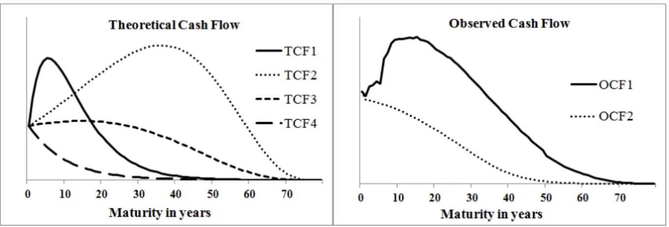
Theoretical cash flows are “typical” in the business, that is, they represent the main profiles that the com-mitments of insurance companies draw over time. It was assumed that the insured portfolio has a history and a number of participants that enable the search for a pat-tern to be designed on the inputs and outputs in cash flow. Thus, four flows with different profiles were simu-lated, namely:
◆ TCF1) Participants in an accumulation phase using only a portion of the accumulated fund for conversion into retirement beneit. he unused fund portion is fully paid back at the conversion time. In this low, there is a conversion concentration around the sixth year and, as a consequence, a cash efort should be made by the insurance company to respond to payback of the un-converted portion, leading the payment curve to have a peak in this region of the graph;
◆ TCF2) Participants in an accumulation phase using only a portion of the accumulated fund for conversion into retirement beneit. he unused fund portion is pe-riodically paid back, in an unscheduled manner, over the concession period. he fact that the payback of the unconverted portion is distributed over time causes a lattening in the payment curve, lengthening the insu-rance company’s debt proile;
◆ TCF3) Participants in an accumulation phase fully using the accumulated fund for conversion into retire-ment beneit. his low enables greater standardization of the payment proile, as it makes a smooth transition between the accumulation and the beneit granting periods, at the time when it turns the entire accumu-lated fund into small paybacks that will take place in the long run;
◆ TCF4) Participants in a beneit granting phase. he pay-ment curve for this low is monotonically decreasing and it represents the depletion of PBMC through the payback of the contracted beneits.
contracts with coverage for survival. In order to preser-ve the business identity of the collaborating company, the flow generation was performed by the company itself from a sample of its portfolio by using premises of its own. Two cash flows were selected for the case study:
OCF1) sampling of active participants, in an accumula-tion phase, from a portfolio with assured yield curve of 6% per year plus IGPM variation and AT49 contractual basis; and OCF2) sampling of assisted participants, in
a concession phase, from a portfolio with assured yield curve of 6% per year plus IGPM variation and AT55 contractual basis. Currently, the insurance contracts with these technical bases are not marketed, however, insurance companies still have relevant liabilities deri-ved from sales in the past. These liabilities are precisely those causing the greatest LAT deficits and insurance companies are particularly interest in them. Figure 2 displays the payment profile of cash flows.
3.1 Svensson's model parameter adjustment.
As the functional relation proposed by Svensson is non-linear, the non-linear regression technique was used to estimate parameters by non-linear least squares. his method uses the derivative of the sum of squared errors (SSE), in relation to the parameters, to guide the search for parameters that minimize SSE. here is no closed so-lution to estimate parameters and the process is iterative. At each iteration, the search direction will be guided by Marquardt’s algorithm. his algorithm was chosen due to its performance in the presence of a high correlation be-tween the estimated parameters; according to Marquardt (1963, p. 439): “While it is not always possible to forsee high correlations among the parameter-estimates when taking data for a nonlinear model, better experimental design can oten substantially reduce such extreme cor-relations when they do occur.” he choice of the initial condition parameters is extremely important for the inal result of this search, because, as it is a non-linear
optimi-zation, one can ind a local minimum, while intending to ind the global minimum. In this context, the appropriate choice of starting values already situates the search algo-rithm within the minimum point neighborhood, some-thing which meets the model’s econometric conditions.
To deine the starting values, we replicated the solution adopted by Diebold and Li (2006) for estimating parameters of the Nelson-Siegel model, which “linearized” the function spot rate s(τ) by setting the non-linear parameter λ, and it estimated the linear parameters β1, β2, and β3 by ordinary least squares. In this research, we arbitrated the non-linear parameters λ1 and λ2 of Svensson’s function spot rate s(τ) and estimated the linear parameters β1, β2, β3, and β4 by ordinary least squares. he set of starting values chosen will be that leading to an adjusted determination coeicient (r2) greater
than or equal to 95%. he proposed modeling is classiied as cross-section, because it uses the interest rate quote observed in a single day to estimate the model parameters. Table 2 dis-plays Svensson’s model estimated parameters.
Parameters Ref Date: 06/29/2012 Ref Date: 12/29/2011 Ref Date: 06/30/2011
IPCA IGPM IPCA IGPM IPCA IGPM
β1 0.04590 0.04140 0.05370 0.05150 0.06150 0.05780
β2 -56.02270 0.16750 0.01510 0.08270 0.06760 -0.09770
β3 56.40380 -0.14310 -0.08820 -0.06420 -0.04310 0.31110
β4 -0.06560 -0.06710 -0.01890 -0.00592 -0.00763 -0.00398
λ1 7.51610 1.60850 0.82970 0.30900 0.27150 1.63120
λ2 0.13180 0.15280 0.14810 0.30900 0.27150 0.08180
SSEinal 9.48E-05 5.580E-05 8.848E-05 6.070E-05 1.732E-04 4.248E-05
1 - SSEinal /
10% 61% 1% 11% 13% 10%
SSEinitial
Table 2 Estimated parameters for Svensson’s model
Source: Prepared by the authors.
3.2 Cubic spline model parameter adjustment.
The solution of the equation system, which leads to a set of cubic spline interpolating polynomials, may be ob-tained by algorithms built for this purpose, easily found in the literature on interpolation. Varga (2000) has pre-sented an algorithm easy to deploy in Visual Basic and it can be turned into a resident function in an Excel spre-adsheet.
As described in Section 2.2.2, the interpolated part of the curve is adjusted by cubic spline, and the extrapo-lated part perpetuates the forward rate, observed within
the last interpolated period, i.e. the last slope observed in the yield curve is kept constant. The forward rate is
determined by: where: Ft,t+1 =
today’s forward rate for the future period between t and
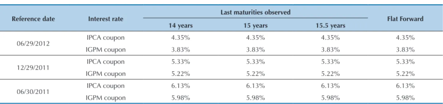
t+1 and St = today’s spot rate for a bond maturing in t. The proposed modeling is classified as cross-section, be-cause it uses the interest rate quote observed in a single day to estimate the model parameters. Table 3 shows the forward rates that were set for extrapolation of each of the six curves fitted by this methodology.
Source: Prepared by the authors.
Reference date Interest rate Last maturities observed Flat Forward
14 years 15 years 15.5 years
06/29/2012 IPCA coupon 4.35% 4.35% 4.35% 4.35%
IGPM coupon 3.83% 3.83% 3.83% 3.83%
12/29/2011 IPCA coupon 5.33% 5.33% 5.33% 5.33%
IGPM coupon 5.22% 5.22% 5.22% 5.22%
06/30/2011 IPCA coupon 6.13% 6.13% 6.13% 6.13%
IGPM coupon 5.98% 5.98% 5.98% 5.98%
Table 3 Rates for the last maturities of the observed yield curve
3.3 Vasicek's model parameter adjustment.
Due to its simplicity and the good results shown for large samples, we used the Moments Method to estimate model parameters. his technique is grounded in the fact that simple sample moments are centered estimators of simple population moments and they consist, primarily, in making equal the sample moment results and the respec-tive equations of population moments. hus, the system solution provides the parameter values. We adjusted the parameters of equations generating average and variance values (irst and second population moments, respective-ly) of the forward rate structure, in order to minimize the squared diferences found in the comparison to the average and the variance values calculated through the observed rates (sample). his comparison is provided for each of the 13 selected maturities of 1, 12, 18, 24, 30, 36, 48, 60, 72, 84, 96, 108, and 120 months, and each maturity consists in a time series of 354 weekly observations (Wednesdays) be-tween 09/21/2005 and 06/27/2012, totaling 4,602 observed points. he proposed technique enables a dynamic moling of the yield curve by capturing the intertemporal de-pendence that may exist in the observed series.
Furthermore, there was a need to choose a proxy for the instantaneous short-term interest rate r, becau-se no bonds with such a short maturity are offered so that it is impossible to know their rates. According to the research methodology, the database used to adjust the model parameters are the interest rates quoted in the DI-IPCA and DI-IGPM swap contracts market traded on BM&FBOVESPA. This market offers contracts with
standardized maturities and the shortest of them is ne-gotiated for a month, which will be used as an instanta-neous proxy for the short-term interest rate r.
he minimization of squared errors is performed throu-gh an initial condition, for the set of parameters, and it will be subject to an iterative process until the minimum point of the error function is found. At each iteration, the search direction will be guided by a quasi-Newton algorithm. he choice of the initial condition of parameters is extremely important for the inal result of this search, because, as it is a non-linear optimization, it is possible to ind a local mini-mum when the intented is the global minimini-mum.
According to Backus et al. (1998), the following as-sumptions were adopted for generating the initial model parameters: the parameter b, the short-term average rate in the long run (equilibrium rate), will be initially set by the average rate of the time series of short-term rates to the one-month maturity (our proxy for the short-term rate
r). he parameter a, the reversal speed in relation to the average value, will be initially be set as the order 1 self--correlation of the short-term time series rates to the one--month maturity. he parameter σ, volatility, will leave the unconditional variance formula σ2 / (1 – a2) when matched
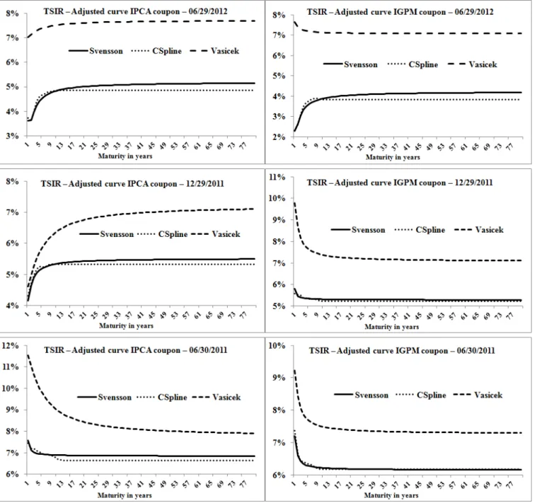
In this section we introduce the main results of this study. hrough the analysis of the six-block graphs, displayed in Fi-gure 3, the yield curves estimated by the models (Svensson’s, cubic spline, and Vasicek’s) were compared, and they will be used in the calculation of current estimates, for the matu-rities ranging from 1 to 80 years. Ater their inspection, it was observed that: (i) diferences in the outline of curves in the interpolated part (maturities between 1 and 15 years) of the forward rate structure spread and they are ampliied in
the extrapolated part (maturities between 16 and 80 years). his detachment in the trajectory of curves over the maturi-ties produces interest rate estimates persistently diferent for a long period; (ii) the rates estimated by the models show diferences that, depending on the payment proile to be dis-counted, have the power to interfere with the current esti-mate results; (iii) the models produce yield curves with tra-jectories of their own that depend, solely, on the architecture employed in their construction.
Interest rate a b σ λ
IPCA coupon 0.97458 0.00553 0.00055 -0.02384
IGPM coupon 0.87099 0.00456 0.00280 -0.06290
Table 4 Estimated parameters for Vasicek’s one-factor model
Source: Prepared by the authors.
4 RESULTS
4.1 Current estimate of theoretical cash flows.
In this section, theoretical cash flows discounted by the TSIR rates built according to the three models dis-cussed in Section 2.2 (these yield curves can be viewed
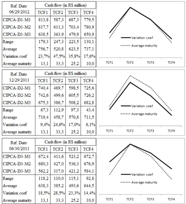
in Figure 3) are shown, something which enables obser-ving the impact that interest rate modeling on the cur-rent estimate of future financial commitments (survival coverage). The results are displayed in Figure 4.
he results displayed in Figure 4 were segmented into three tables, based on the reference dates used in yield curve modeling: 06/29/2012 (D1), 12/29/2011 (D2), and 06/30/2011 (D3). he tables were arranged into 3 rows and 4 columns, with lines indicating the TSIR model used to low discount (Svensson’s (M1), cubic spline (M2), and Vasicek’s (M3)) and columns indicating the low proile in the theo-retical cash that was discounted (TCF1, TCF2, TCF3, and TCF4). hus, each table provides a set of 12 current estima-tes for each of the daestima-tes used to generate the yield curves. As
the cash lows are theoretical, they may it any reference date. Were performed 2 analyses: one vertical, on the sense of cash flows, checking the current estimate sensitivity to choice of the yield curve model, and another horizon-tal, on the sense of models, checking the current estima-te sensitivity to choice of the payment profile.
he vertical analysis of results on 06/29/2012 indi-cates that the current estimate is sensitive to choice of the model. We observed that amplitude ranged between 130.1 million (variation coeicient of 17.6%) and 247.3 Source: Prepared by the authors.
million (variation coeicient of 47.5%). A dispersion in this magnitude indicates that, on the one hand, the cur-rent estimate calculated with the model rates situated at the lower end of the amplitude could be accommodated within liabilities constituted by the insurance company (NCA) without generating a lack of provisions (LAT). On the other hand, the current estimate calculated with mo-del rates situated at the upper end of the amplitude, could extrapolate the liabilities set up, indicating insuiciency of provisions. hat is, we could have a reversal in the LAT result, depending on the model chosen to build the TSIR.
he main conclusion of the horizontal analysis (in re-lation to the results sensitivity to choice of models) for 06/29/2012 may be viewed in the graph attached to the ta-ble in Figure 4: the correlation between the proile of cash low, according to its average maturity, and the dispersion of current estimate caused by the models, according to the variation coeicient. his direct relation between me-asures indicates that the impact of model choice on the
current estimate will be higher when the cash low proile is longer. hus, it may be concluded that cash lows with concentration of payments in longer maturities (long pro-ile) sufer, more intensely, the efect of interest rates sha-ped by diferent techniques. his efect is aggravated by the detachment that can occur between the trajectories of the yield curves in extrapolated maturities (longer).
he analyses for the reference dates 12/29/2011 and 06/30/2011 are conducted in a similar manner and, throu-gh the symmetry of results displayed in Figure 4, indings similar to the analysis of the reference date 06/29/2012 were obtained for: the current estimate is sensitive to choice of model used to build the TSIR and this sensitivity increases with the longevity of the cash low that is being discounted.
Next, we analyzed the efect that the change in the refe-rence date has on the current estimate. Table 5 displays the results of the current estimate according to reference date and payment proile. From Figure 4, the current estimate of the “average” line was extracted.
Source: Prepared by the authors.
Current estimate (R$ million) TCF1 TCF2 TCF3 TCF4
Reference date 1 - 06/29/2012 756.7 520.8 623.5 737.1
Reference date 2 - 12/29/2011 719.4 458.7 570.8 711.5
Reference date 3 - 06/30/2011 638.3 385.2 493.6 644.5
Range 118.4 135.6 129.9 92.6
Table 5 Current estimate (IPCA coupon) of theoretical cash flows
he results in Table 5 indicate that the current estimate is sensitive to choice of the date on which the TSIR was built. Indeed, as the cash lows do not change and a typical yield curve was used, built having quoted rates as a basis in each of the three reference dates, the diferences are due to oscillation that the ixed income market and its derivatives showed over time. It may be said that even if the designed future commitments (cash lows) of an insurance company do not change from one date to another (simplifying hypo-thesis), the current estimate will be an uncertain value, as it depends on macroeconomic factors (inlation expecta-tions, economic activity level, and others) observed on the date when the TSIR, used to discount cash lows, is built.
Finally, the analysis of results indicates that: (i) the current estimate is sensitive to choice of the model used to build the TSIR; (ii) this sensitivity increases with the longevity of the cash low that is being discounted; (iii)
the current estimate is an uncertain value in time, since the TSIR depends on macroeconomic factors prevailing at the time of its construction.
4.2 Liability adequacy test of observed cash
flows.
In order to analyze the impact that the interest rate modeling produces on the current estimate of future fi-nancial commitments arising from the guarantees offe-red in insurance with survival coverage, we applied the LAT. Thus, observed cash flows (described in section 3) were discounted by the rates of TSIR constructed accor-ding to the three models discussed in section 2.2, com-pared with their respective established technical provi-sions (given that it is a portfolio of real insurance).
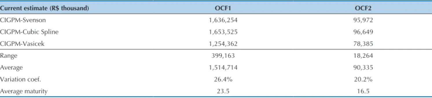
Table 6 displays the current estimate results of the cash flow designed.
Source: Prepared by the authors.
Current estimate (R$ thousand) OCF1 OCF2
CIGPM-Svenson 1,636,254 95,972
CIGPM-Cubic Spline 1,653,525 96,649
CIGPM-Vasicek 1,254,362 78,385
Range 399,163 18,264
Average 1,514,714 90,335
Variation coef. 26.4% 20.2%
Average maturity 23.5 16.5
As we can observe in Table 6, the current estimate discounted by the rate modeled by cubic spline is at the upper end of the amplitude for the two flows, while the current estimate discounted by the rate modeled by Va-sicek is at the lower end of the amplitude, for both flows, too. This suggests that the spline cubic model is more conservative than the other models tested. As the tests were not exhaustive and/or they have not been proven algebraically, it is not possible to claim the spline cubic model is always more conservative, but only that there is evidence of it. We also found that the portfolio of active participants (OCF1), which has a longer payment profile
(average maturity of 23.5 years), had a higher dispersion (variation coefficient of 26.4%) than the portfolio of as-sisted participants, which has a shorter payment profile (average maturity of 16.5 years) with a variation coeffi-cient of 20.2%. Similarly, the results suggest that cash flows with concentration of payments on longer matu-rities (long profile) suffer, more intensely, the effect of interest rate model choice. This effect is aggravated by the detachment that can occur between models, related to the trajectory of the yield curves in the extrapolated maturities (longer).
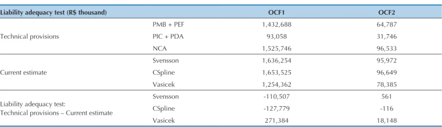
Finally, Table 7 summarizes the LAT results.
Liability adequacy test (R$ thousand) OCF1 OCF2
Technical provisions
PMB + PEF 1,432,688 64,787
PIC + PDA 93,058 31,746
NCA 1,525,746 96,533
Current estimate
Svensson 1,636,254 95,972
CSpline 1,653,525 96,649
Vasicek 1,254,362 78,385
Liability adequacy test:
Technical provisions – Current estimate
Svensson -110,507 561
CSpline -127,779 -116
Vasicek 271,384 18,148
Table 7 Liability adequacy test of cash flows observed on 12/29/2011
Source: Prepared by the authors.
he analysis of the current estimate had already sho-wn that the spline cubic model was the most conservative and, therefore, it might be expected that its discounted low required more resources from the company in the LAT, so-mething which really happened. he same reasoning may be applied to Vasicek’s model that, being less conservative, might require fewer resources from the company. he most important conclusion of this test is that the choice of model used to estimate the TSIR can reverse the LAT result. For the cash low of active participants (OCF1), Svensson’s and
the cubic spline models indicate an insuicient provision, while Vasicek model of points out a suicient one. For the cash low of assisted participants (OCF2), the spline cubic model indicates an insuicient provision, while the others point out a suicient one.
The analysis of results indicate that: (i) the LAT result is sensitive to choice of model used to build the TSIR; (ii) the LAT is an uncertain value in time, as the TSIR depends on the macroeconomic factors prevailing at the time of its construction.
5 FINAL REMARKS
According to the methodology used in this study, the effect of choosing between the spline cubic, Svensson’s, and Vasicek’s models was analyzed to fit the yield curve (TSIR), in the current estimate of actuarial liabilities and in the LAT.
The results suggest that: (i) the LAT is sensitive to choice of the model used in the construction of the TSIR; (ii) this sensitivity increases with the cash flow longevity, as the current estimate is sensitive to the ave-rage maturity of payments inherent to the flow; (iii) the LAT is an uncertain value in time, as the TSIR depends on macroeconomic factors prevailing at the time of its construction.
an investor requires to exchange a short-term position for another one, on the long run) and the expected long-term nominal convexity efect (a purely technical efect which re-presents the non-linear relation between the interest rate and the price of a bond). he assessment of technical provisions, with values designed on such a long-term horizon, justiies the adoption of this parameter that, although controversial, is economically feasible and equalizes the ultimate forward inancial assumptions. Given the scope of this subject and the excessive space it approach demands, we chose this brief discussion so that the reader may become aware of its im-portance in this context.
Therefore the results obtained reinforce the warning related to the choice of the most appropriate model for obtaining the rate to be used in the liability adequacy test, as it can severely affect the solvency and performan-ce indicators of insuranperforman-ce companies. For accounting purposes, this choice is critical and confirms the need to properly justify the criteria that guided the recogni-tion and measurement of the elements, especially in a principle-based accounting, as in the case of the IFRS, in which the discretion allowed to the person in charge im-plies, by contrast, the responsibility to properly account for the criteria adopted to support the choices.
Agliata, F., Maglio, R., Ferrone, C., & Tuccillo, D. (2011). he evolution of the IASB insurance project and the possible relections in the inancial statements of insurance companies. Available at http://ssrn.com/ abstract=1985246
Associação Brasileira das Entidades dos Mercados Financeiro e de Capitais. (2010). Estrutura a termo das taxas de juros estimada e inlação implícita metodologia. Available at http://portal.anbima. com.br/informacoes-tecnicas/precos/ettj/Documents/est-termo_ metodologia.pdf
Backus, D., Foresi, S., & Telmer, C. (1998). Discrete time models of bond pricing (Working Paper 6736). Cambridge: NBER. Available at http:// www.nber.org/papers/w6736.pdf
Banco Central do Brasil. (2014, agosto). Decompondo a inlação implícita (Trabalhos para Discussão n. 359). Brasília, DF: BCB. Available at http://www.bcb.gov.br/pec/wps/port/TD359.pdf
Bank for International Settlements. (2005). Zero-coupon yield curves:
technical documentation (Papers, 25). Basel: BIS. Bolder, D. J. (2001). Aine term-structure models: theory and
implementation (Working Paper 2001-15). Ottawa: Bank of Canada. Available at http://www.bankofcanada.ca/wp-content/ uploads/2010/02/wp01-15a.pdf
Bostan, I. (2011). Implications of European directives in the assessment of insurance companies. heoretical and Applied Economics, 18(3), 131-140.
Committee of European Insurance and Occupational Pensions
Supervisors. (2010). Solvency II calibration paper. Frankfurt: CEIOPS. Culbertson, J. M. (1957, novembro). he term structure of interest rates.
he Quarterly Journal of Economics, 71(4), 485-517.
Diebold, F. X., & Li, C. (2006, fevereiro). Forecasting the term structure of government bond yields. Journal of Econometrics, 130(2), 337-364. Franklin Jr., S. L., Duarte, T. B., Neves, C. R., & Melo, E. F. (2011).
Interpolação e extrapolação da estrutura a termo de taxas de juros para utilização pelo mercado segurador brasileiro. Available at http://www.susep.gov.br/download/menumercado/artigo_ETTJ_ CORIS_15032011.pdf
Gasha, G., He, Y., Medeiros, C., Rodriguez, M., Salvati, J., & Yi, J. (2010). On the estimation of term structure models and an application to
the United States. International Monetary Fund, Working Paper
WP/10/258.
Lindberg, D. L., & Seifert, D. L. (2010). A new paradigm of reporting on the horizon: International Financial Reporting Standards (IFRS) and implications for the insurance industry. Journal of Insurance Regulation, 29(2), 229-252.
Mano, C. C. A., & Ferreira, P. P. (2009). Aspectos atuariais e contábeis das provisões técnicas. Rio de Janeiro: Funenseg.
Marquardt, D. W. (1963, junho). An algorithm for least-squares estimation of nonlinear parameters. Journal of the Society for Industrial and Applied Mathematics, 11(2), 431-441.
Nelson, C. R., & Siegel, A. F. (1987, outubro). Parsimonious modeling of yield curves. Journal of Business, 60(4), 473-489.
Post, T., Gründl, H., Schmidl, L., & Dorfman, M. S. (2007). Implications of IFRS for the European insurance industry: insights from capital
market theory. Risk Management and Insurance Review, 10(2),
247-265.
Superintendência de Seguros Privados. (2012). Seguradoras: provisões detalhadas. Rio de Janeiro: SUSEP. Available at http://www2.susep.gov. br/menuestatistica/SES/principal.aspx
Superintendência de Seguros Privados. (2013). 1o Relatório de Análise
e Acompanhamento dos Mercados Supervisionados. Rio de Janeiro: SUSEP. Available at http://www.susep.gov.br/setores-susep/ cgpro/relatorios-analise-acompanhamento/Relatorio_Mercados_ Supervisionados_SUSEP.pdf
Svensson, L. E. O. (1994). Estimating and interpreting forward interest rates: Sweden 1992-1994 (Working Paper 4871). Cambridge: NBER, 1994. Varga, G. (2000). Interpolação por cubic spline para a estrutura a termo
brasileira (Resenha BM&F n. 140). São Paulo: BM&F.
Varga, G. (2009). Teste de modelos estatísticos para a estrutura a termo no Brasil. RBE, 63(4), 361-394.
Vasicek, O. A. (1977, novembro). An equilibrium characterization of the term structure. Journal of Financial Economics, 5(2), 177-188.
Correspondence Address: Antonio Aurelio Duarte
Fundação Escola de Comércio Álvares Penteado Avenida Liberdade, 532 – CEP: 01502-001 Liberdade – São Paulo – SP