Survey sampling for fisheries monitoring in Brazil: implementation and
analysis
Census of ishing data about the landings carried
out along the São Paulo coast during 2011 was
used to evaluate and compare the survey sampling
for isheries monitoring, expecting reliable
results along with an important cost reduction.
Estimates of total catch for the São Paulo State
as a whole and by municipality were relatively
accurate (high precision and low bias). Estimated
catch by month, by ish categories and both
(factors not considered in the sampling design)
demonstrated that, as the level of required
detail increased, the catch estimates became
more biased and less precise. However, when
comparing to the 2011 true catches, the order of
importance of ish categories based on estimated
catches changed slightly in some positions after
the ifth place. There was a minor cost reduction
due to the sampling in comparison with the census
methodology currently in use (15.4% at most).
The results demonstrated that isheries monitoring
costs are directly proportional to the required level
of details and data quality.
AbstrAct
Laura Villwock de Miranda
1,5*, Paul Gerhard Kinas
1,2, Guilherme Guimarães Moreira
3#, Rafael
Cabrera Namora
4, Marcus Henrique Carneiro
51 Programa de Pós-Graduação em Oceanograia Biológica, Universidade Federal do Rio Grande (FURG). (Av. Itália, km 8, Carreiros, 96203-900, Rio Grande, RS, Brazil).
2 Instituto de Matemática, Estatística e Física (IMEF/FURG). (Av. Itália, km 8, Carreiros, 96203-900, Rio Grande, RS, Brazil). 3 Instituto Brasileiro de Geograia e Estatística (IBGE).
(Rua Oliveira, 523, 4th loor, Cruzeiro, 31310-150, Belo Horizonte, MG, Brazil). 4 Fundação de Desenvolvimento da Pesquisa do Agronegócio (FUNDEPAG) (Rua Dona Germaine Burchard, 409, Água Branca, 05002-062, São Paulo, SP, Brazil). 5 Instituto de Pesca de São Paulo (IP/APTA-SP)
(Rua Joaquim Lauro de Monte Claro Neto, 2275, Itaguá, 11680-000, Ubatuba, SP, Brazil).
*Corresponding author: [email protected]
Descriptors:
Fishing activity, Fishing landings,
Sampling design, Inference, Monitoring costs.
Informações sobre as descargas pesqueiras realizadas em
2011 ao longo da costa de São Paulo foram utilizadas com
o objetivo de avaliar e comparar os métodos de
amos-tragem em campanhas voltadas para o monitoramento
pesqueiro. Espera-se com isto um conjunto de dados
con-sistentes, além de uma importante redução de custos. As
estimativas da captura total para o estado de São Paulo e
por municípios foram relativamente acuradas (alta
preci-são e baixo viés). A captura estimada por mês, por
catego-ria de pescado e por ambos (domínios não considerados
no desenho amostral) demonstraram que quanto maior é
o nível de detalhamento menos precisas e mais enviesadas
tornam-se as estimativas de captura. Quando comparada
com as capturas reais para 2011, a ordem de importância
das categorias de pescado baseada nas capturas estimadas
alterou-se ligeiramente em algumas posições após o
quin-to lugar. Houve uma pequena redução de cusquin-tos devido à
amostragem em comparação com a metodologia
censitá-ria atualmente em uso no estado de São Paulo (máxima de
15,4%). Os resultados demonstraram que os custos do
mo-nitoramento pesqueiro são diretamente proporcionais ao
nível de detalhamento e à qualidade dos dados requeridos.
resumo
Descritores:
Atividade pesqueira, Descargas
pesqueiras, Desenho amostral, Inferência,
Cus-tos de monitoramento.
http://dx.doi.org/10.1590/S1679-87592016132706404
INTRODUCTION
Catch and ishing efort are the most basic information that can be obtained about any ishing activity. To guarantee that at least these data are reliably collected and maintained over time is crucial to formulate efective isheries policies and management plans (HILBORN; WALTERS, 1992; CADIMA, 2003).
Monitoring and obtaining ishing information can be performed in two forms: by sampling surveys (CADDY; BAZIGOS, 1985; ARAGÃO; MARTINS, 2006; LIMA-GREEN; MOREIRA, 2012) or by census (FAO, 1999; MENDONÇA; MIRANDA, 2008; ÁVILA-DA-SILVA et al., 2015). In general, a census is recommended when the population is small, sampling errors are large, information is cheap to obtain or the cost in making the wrong decisions is high. Sampling techniques must be used when the population is very large and/or the cost (concerning money and time) to obtain information is high (CADDY; BAZIGOS, 1985; BOLFARINE; BUSSAB, 2005).
When the available data constitute only a portion of a population (collected by sampling), then there are two ways of dealing with the inferences: (1) based on a sampling plan specially designed by a inite population with a controlled random selection procedure where all probabilities involved can be known (design-based); and (2) based on observational research (model-based), where there is no control over the sampling plan and the speciication of a model plays a fundamental role to connect the observed data to the parameters of the population (COCHRAN, 1977; BUSSAB; MORETTIN, 2012). Basically, in a model-based approach, data are assumed to have been generated from a random process speciied by a probability model so that conclusions can be generalized to other situations where the same process operates, while design-based inference cannot be generalized to other populations which were not sampled (LUMLEY, 2010).
The design-based approach is usually applied to the analysis of complex survey samples and, up to now, widely adopted by isheries monitoring methodologies (FAO, 1999). Estimates of total catch, their variance and any other population quantities are obtained based on the Horvitz-Thompson estimator (HORVITZ; THOMPSON, 1952). This is an unbiased estimator of population total applicable to any sampling design with or without replacement, from a inite population, when unequal but known selection probabilities are used. The estimation
procedure weighs each selected unit by the inverse of its overall selection probability and known nonzero pairwise probabilities are required for unbiased variance estimation (LUMLEY, 2010).
Historically, isheries monitoring in Brazil has certainly been inluenced by diferent political and institutional arrangements made along the development of national extractive ishery (DIAS-NETO, 2010, 2011; LIMA-GREEN; MOREIRA, 2012). The adoption of diferent methodologies for diferent isheries or for the same ishery in time has been common, with periods of interruption in data collection in diferent regions along the Brazilian coast.
In some States of Brazil, the EstatPesca (ARAGÃO; MARTINS, 2006) was the most adopted sampling methodology for isheries monitoring since the nineties (LIMA-GREEN; MOREIRA, 2012). This methodology was based on the follow-up of ixed samples of ishing vessels, which required a permanently updated registry of all vessels in operation. This proved impracticable, mainly for small-scale isheries, where sales and changes in the names and in the characteristics of the vessels are very frequent. It was also usual that vessel sampling was intentionally motivated by logistics considerations and not conducted as a probabilistic sampling survey and, therefore, subjected to bias (ISAAC et al., 2008). In order to reduce biased estimates, more samples should be taken, increasing the costs of the sampling process. ISAAC et al. (2008) observed a catch overestimation when EstatPesca was applied to the isheries monitoring of the Pará State (Northern Brazil) and concluded that at least 70% of the leet should be sampled to place the error of the estimates at acceptable levels.
target species, besides ishing landings with small catches spread over large extensions of the coast are some of the characteristics described for small-scale ishing in Brazil (ISAAC et al., 2000, 2008; MENDONÇA; MIRANDA, 2008). Furthermore, when the IBGE methodology is applied with a two stages sampling, the total numbers of landings carried out in a ishing lading place must be known. This information can be very diicult to be obtained and, of course, it is not known in advance. Many factors can inluence the dynamics of ishing landings, such as the size of the landing facility, the number of ishing vessels and ishermen at this facility, the ishing seasons, the type of ishing leet and the ishing gears used by this leet.
Fisheries monitoring of the São Paulo coast is, however, an exception in Brazil and its irst records of ishing information dates back to 1944. Since its creation in 1969, the Fisheries Institute of the Department of Agriculture and Food Supply of São Paulo State has been the institution responsible for the collection, storage, processing and disclosure of census data (FAO, 1999) about the marine isheries production landed along the São Paulo coast (MENDONÇA; MIRANDA, 2008; ÁVILA-DA-SILVA et al., 2015).
Realistic and good quality data, where the true total population is known, are required to evaluate and compare survey sampling methods (LUMLEY, 2010). In this paper, the complete ishing data of São Paulo State collected during 2011 were used to simulate probability samples following the sampling design described by LIMA-GREEN and MOREIRA (2012) and to compare the results of these simulations to the true total landed catches. In addition to the quality of estimates, the costs to perform isheries monitoring on the São Paulo coast were also considered in order to evaluate losses and gains of the sampling methodology when compared to census data collection. The hypothesis of this study is that the survey sampling method applied to isheries monitoring of the São Paulo coast will generate reliable results along with an important cost reduction when compared to the census data collection.
MATERIAL AND METHODS
Obtaining fishing information
Fishing landings census data collected on the São Paulo coast during 2011 were used to apply the sampling methodology for isheries monitoring proposed by
IBGE (LIMA-GREEN; MOREIRA, 2012). These data were obtained through the Fishing Activity Monitoring Program (PMAP), coordinated by isheries scientists from the Fisheries Institute of the Department of Agriculture and Food Supply of São Paulo State.
In March 2008, PMAP began to be used aiming to evaluate the impact on ishing activity by oil and gas exploration activities by Petrobras in the Santos Basin. The PMAP applies the census methodology to collect isheries statistics (FAO, 1999; MENDONÇA; MIRANDA, 2008; ÁVILA-DA-SILVA et al., 2015), and currently monitors 196 ishing ports and landing places (just “ports” in the remaining text) in 15 municipalities included in the area of inluence of the oil and gas exploration in Santos Basin. The municipality of Santos has only one port and was considered a single municipality together with the neighboring city of Guarujá to preserve the conidentiality of information. In order to obtain information on catch and ishing efort, ield agents perform structured interviews with ishermen on the occasion of landing. This information is complemented with retrieved ishermen’s records about their daily ishing operations (self-registration), in logbooks and with records provided by ishing enterprises. The storage, processing, analysis and provision of ishery statistics are carried out by the System Manager ProPesq®
(ÁVILA-DA-SILVA et al., 1999), currently operating in a web platform, called ProPesqWEB (http://www.propesq. pesca.sp.gov.br).
Applying sampling methodology to
fisher-ies monitoring
The organization and structuring of ishing landings census data of the State of São Paulo and the sampling design to extract ishing landings from it were deined during a Workshop with technicians of IBGE, who are the authors of the methodology being validated (LIMA-GREEN; MOREIRA, 2012).
The registry of ports
(fewer than one weekly landing); (2) Reconsider all ports with at least one landing greater than 500 t; (3) Gather in a single port all places which, for logistics, have distinct names in the database, but in practice could be part of only one port; (4) Remove from the registry, the ports that were deactivated in 2013. After accomplishing these steps, the register was inalized with a total of 133 ports located along the entire coast of Sao Paulo State (Figure 1).
of Itanhaém, São Vicente and Bertioga have three or fewer ports and therefore all of them comprised the census stratum. Any port with unmatched speciicity in landings, when identiied, was transferred to the census stratum because it could cause distortions in later sample expansion.
Expansion and statistical inference
All estimates of this study were obtained through software R (R CORE TEAM, 2015) using package Sampling (TILLÉ; MATEI, 2015) for the port sampling and package Survey (LUMLEY, 2014) for the estimate calculations. The sample sizes were deined to be two ports, randomly chosen, in strata with up to six ports and three ports for all others. Therefore, a total of 77 ports composed the sample, 36 in the census strata and 41 in the sampled strata. Main equations used in this analysis are speciied in Table 1.
This study performed 100 simulations, each containing the sample selection of ports and total catch estimation for each one of the 14 municipalities of São Paulo. For each of the 100 simulations, the estimated total landed catch by municipality (Yi
k
Q V
[ – Equation 10) and associated standard error (SEiQ Vk– Equation 3), the coeicient of variation
(CViQ Vk– Equation 4), the square root of the mean squared
error (RMSEi k
Q V – Equation 17), the percentage bias (% Bi
k
Q V– Equation 5) with respect to the true total landed
catch of 2011 (Yi– Equation 7), and the design efect
(DeffiQ Vk– Equation 18) were calculated. Furthermore, the
annual economic cost of isheries monitoring, obtained as a sum of costs for sampled ports, was also obtained in each simulation. The R package Survey (LUMLEY, 2014) estimates standard errors (SE) as the square root of the Horwitz-Thompson estimated variance of the total population, and was implemented with the option ’ultimate cluster’ method (Equation 13). The best sample allocation of ports within each municipality was chosen from the 100 simulations under two criteria: Sampling Plan 1 (SP1) - the sample with the lowest RMSE; Sampling Plan 2 (SP2) - the sample with the lowest economic cost. It is important to clarify that whenever referring to accuracy or to an accurate estimate in the remaining text, the compromise between the variance and the squared bias of the estimate will be considered (low RMSE).
The inal estimate of the total catch by municipality (Yi
k
Q V \
– Equation 19) was obtained by a simple average of the 100 simulated estimates and the coeicient of variation (CVi) was calculated from its standard error
Figure 1: Location of ishing ports and landing places monitored in 2011 on the coast of São Paulo, Brazil included in the register (population of interest) for the analysis.
Sampling design based on catch information
The IBGE methodology is based on a complex sampling design, composed of stratiication of the ports and conglomeration of landings within ports for the calculation of total catch estimates and their associated sampling errors or coeicients of variation. This study assumed a single conglomerate sampling design, i.e., the information of all landings carried out at sampled ports was considered in the analysis.
According to LIMA-GREEN and MOREIRA (2012), the ports should be previously divided into strata regarding their importance. One stratum called census stratum was composed of ports selected arbitrarily by their importance, according to historical total landed catches. For all others, called sampled strata, simple random samples (without replacement) of ports were used.
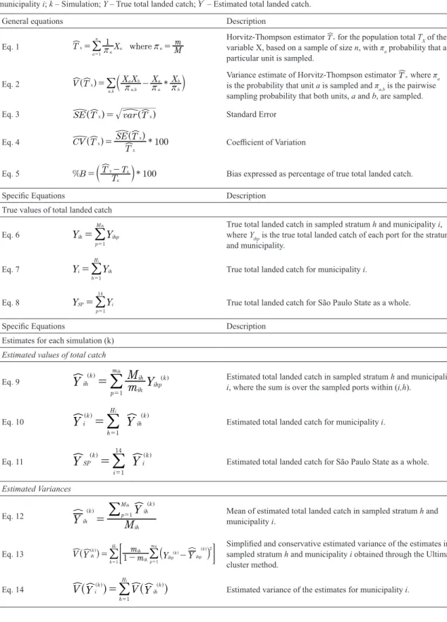
Table 1. Main equations used to obtain estimated total catch and its measures of variability and bias by municipalities and
total of São Paulo State. A – Symbology; i – Municipality; p – Port; h – Stratum; Hi – Total number of sampled strata in municipality i; Mih – Total number of ports in sampled stratum h and municipality i; mih – Total number of sampled ports in sampled stratum h and
municipality i; k – Simulation; Y – True total landed catch; Y{ – Estimated total landed catch.
General equations Description
Eq. 1 Tx 1 X where Mm
a a n a a 1r r = = =
{
/
Horvitz-Thompson estimator Tx
{ for the population total TX of the
variable X, based on a sample of size n, with πa probability that a
particular unit is sampled.
Eq. 2 V T X X X * X
, , x a b a b a a b b a b r r r
=
-Q V T Y
{ {
/
Variance estimate of Horvitz-Thompson estimator T{x where πa is the probability that unit a is sampled and πa,b is the pairwisesampling probability that both units, a and b, are sampled.
Eq. 3 } {SE TQ xV= var T} {Q xV Standard Error
Eq. 4 CV T *
T SE T 100 x x x =
Q V Q V
} { }{{ Coeicient of Variation
Eq. 5 %B T T T *100 x
x x
=T{ - Y Bias expressed as percentage of true total landed catch.
Speciic Equations Description
True values of total landed catch
Eq. 6 Yih Yihp p M 1 ih = =
/
True total landed catch in sampled stratum where Yihp is the true total landed catch of each port for the stratum h and municipality i, and municipality.Eq. 7 Yi Yih h H 1 i = =
/
True total landed catch for municipality i.Eq. 8 YSP Yi p 1
14
=
=
/
True total landed catch for São Paulo State as a whole.Speciic Equations Description
Estimates for each simulation (k)
Estimated values of total catch
Eq. 9
Y
ihm
M
Y
k ih ih p m ihp k 1 ih
=
=QV QV
{
/
Estimated total landed catch in sampled stratum h and municipality i, where the sum is over the sampled ports within (i,h).Eq. 10
Y
iY
k h H ih k 1 i
=
= QV QV{
/
{
Estimated total landed catch for municipality i.Eq. 11
Y
SPY
k i i k 1 14
=
= QV QV{
/
{
Estimated total landed catch for São Paulo State as a whole.Estimated Variances
Eq. 12
Y
M
Y
ih k ih ih k p M 1 ih=
=QV QV
|
/
{
Mean of estimated total landed catch in sampled stratum h andmunicipality i.
Eq. 13 V Yih 1mm Y Y
k ih ih ihp k ihp k p m h H 2 1 1 ih i = - -= =
R Q S Q Q
W X
V V V
# &
{ {
/
/
| Simpliied and conservative estimated variance of the estimates in sampled stratum h and municipality i obtained through the Ultimatecluster method.
Eq. 14
V Y
iV Y
k h H ih k 1 i
=
=R QVW R QVW
Eq. 15
V Y
SPV Y
k i i k 1 14=
=R QVW R QVW
{ {
/
{ {
Estimated variance of the estimates for São Paulo State as a whole.Other deinitions
Eq. 16
B
iY
Y
k i
k i
=
R
-QV
{
QVW
Bias of the estimates for municipalityi.
Eq. 17
RMSE
iV Y
B
k
i k
i k 2
=
R+
Q
QV
{ {
QVW QVV
Squared root of the mean squared error of the estimates for muni-cipality i.Eq. 18
Deff
V
Y
V Y
i k srs i k i k=
R R Q Q Q W W V V V{
{ {
{
Design Efect of the estimates for municipality i, where Vsrs Yi k R QVW { { is the estimated variance of a simple random sample of landings of the same size.
Estimates with all 100 simulations
Eq. 19
Y
Y
100
i k k 1 100=
= Q V|
/
{
Mean of estimated total landed catch obtained as a simple average of 100 simulated estimates of the total catch for municipality i.Eq. 20
V Y
Y
Y
100
1
i i k k 2 1 100=
=-
-R
W
R QV W{ {
/
{
|
Variance of the mean of estimated total landed catch of 100 simulations for municipality i.(SEi - Square root of V YR Wi
[ \ – Equation 20). The coverage
of the conidence interval (1-α=0.95) (CI95) was obtained by counting the samples (simulations) for which the true landed catch (Yi) was encompassed by the CI95.
Obtaining fisheries monitoring costs
Information gathered by the PMAP was used to obtain: the cost for monitoring each port, the total cost for each sample by adding over the costs of its set of ports and also to select the best sample according to SP2.
In PMAP, distant ports are monitored through regular ield trips using institutional or private vehicles. Although the combination of ports monitored per trip can vary for diferent reasons, to simplify, the cost calculation assumed individual trips to each port. The cost of fuel (in liters/ month) per port was obtained based on the distance traveled (round trip), weekly frequency of monitoring and fuel consumption (l/km) in accordance with the type of vehicle (car, motorcycle or boat). Other costs include wages, equipment, supply and maintenance, food and lodging and services like database and computers maintenance, printing and telephony and were all used to obtain the cost of each employee.
Depending on the number and set of ports to be monitored, the number of monitors (supervisors), ield agents and typists varies. Aiming at a lower cost, the number of ield agents in SP2, compared to SP1, was reduced. The number of typists was based on the total number of hours required to include all landings from
the set of sampled ports, which considered the number of reported landings and the ability to include 20 landings per hour into the database. Typing cost by port considered the inclusion cost by landing into the database (total cost with typists divided by the total number of landings times the number of landing per port). The total cost of each remaining employee was divided by the attended ports under his/her responsibility. Expenses related to the coordination and management of the PMAP, despite being overhead costs, were also considered and equally divided between ports that comprised each sampled set. The calculations were based on the highest wage for each position and did not include the administration fees.
RESULTS
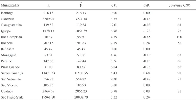
The estimated total catch per municipality was obtained together with the associated coeicient of variation, percentage bias and CI95 coverage (Table 2). For municipalities with few ports (Bertioga, Itanhaém and São Vicente), all ports were allocated in the census stratum and the dispersion measures were therefore equal to zero. Estimates of the total landed catch in all remaining municipalities had low bias, but the maximum CV among samples was obtained in Caraguatatuba (12.0%). The coverage of the CI95 has not encompassed the true value of catches in 95% of samples as it should, except for Ilha Comprida where the coverage was complete (100%).
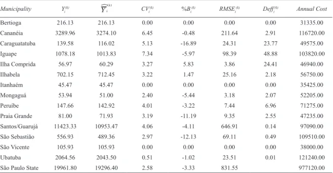
was chosen (Table 3). The estimates with the highest variability (CV) were obtained in the municipalities of Caraguatatuba, Iguape, Ilha Comprida, Mongaguá, Praia Grande and São Sebastião, which also presented values of design efect (Def) greater than one, indicating that the stratiication made between ports for these municipalities did not improve in comparison to simple random sampling. Caraguatatuba had estimates with the highest values of CV and bias. The best results were found for Ubatuba.
In Table 4, similar inference results are shown for the selected set of ports for each municipality providing the lowest monitoring cost (SP2). Catch estimates were less accurate than those found for SP1, which is demonstrated by the higher CV value and RMSE for virtually all municipalities (except for Caraguatatuba and Ilha Comprida that had equal values).
The results that will be presented from now on, and in more detail, refer only to the set of ports by municipality resulting in the smallest RMSE (SP1). After obtaining the estimates of total catch per municipality, some other domain estimations (month and ish categories) that were not considered in the sampling design, were made.
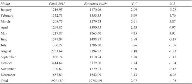
Monthly catch estimates for São Paulo State as a whole and associated dispersion measures are displayed in Table 5. Despite the relatively accurate estimates, the worst results were observed in February (largest CV) and November (largest bias).
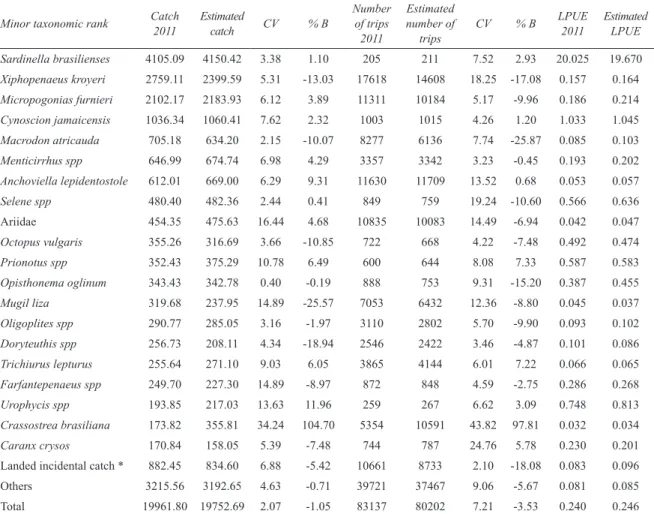
Fish categories landed on the São Paulo coast over 2011 (identiied at minor taxonomic rank possible during data collection) were also considered as domain to compute the catch estimates (Table 6). The 20 most important ish categories (in relation to landed catch) have been listed. All remaining categories have been lumped together in “Others”. Incidental landed catches have also been included in the analysis. Considering CV and
bias, Crassostrea brasiliana and Opisthonema oglinum
were the species with the worst and the best estimates of catch, respectively. In relation to the estimated number of trips, C. brasiliana had the worst estimates again while
Menticirrhus spp had the best results. The CV of estimated
number of trips by ish category tended to be greater than the CV of estimated catch. With this information, the estimated LPUE (reported Landed catch Per Unit of Efort, kg*trip-1) calculated for 2011 was compared to the
true LPUE and few diferences were observed (Table 6). When comparing estimated and actual catches for 2011, it was found that the order of importance of ish categories in landings of São Paulo has remained the same for the irst four categories and showed a slight diference in some of the remaining positions (Figure 2). Only Macrodon
atricauda, Octopus vulgaris, Mugil liza and Doryteuthis
spp were ranked worse than actual order by two or more positions while C. brasiliana was the only category really
badly ranked, with eight positions higher than actual order.
Table 2. Results obtained by simple average between 100 estimates of the total catch (tons) by municipality for São Paulo coast over 2011. Yi – True total landed catch (tons); Y{i – Estimates of total landed catch (tons); CVi - Coeicient of variation between averages; %Bi
– Bias expressed as percentage of catch 2011.
Municipality Yi Yi{ CVi %Bi Coverage CI95
Bertioga 216.13 216.13 0.00 0.00
Cananéia 3289.96 3274.14 3.85 -0.48 81
Caraguatatuba 139.58 139.54 12.01 -0.03 68
Iguape 1078.18 1064.39 6.98 -1.28 77
Ilha Comprida 56.97 56.60 4.89 -0.65 100
Ilhabela 702.15 703.85 2.19 0.24 56
Itanhaém 45.47 45.47 0.00 0.00
Mongaguá 53.94 53.88 4.96 -0.10 67
Peruíbe 147.66 147.44 3.26 -0.15 66
Praia Grande 81.00 80.37 6.04 -0.78 86
Santos/Guarujá 11423.33 11500.55 5.43 0.68 90
São Sebastião 556.93 554.27 9.20 -0.48 71
São Vicente 105.93 105.93 0.00 0.00
Ubatuba 2064.56 2066.23 0.98 0.08 81
Table 3: Results of the Sampling Plan 1 (SP1) – the lowest square root of the mean squared error (RMSE) – by municipality
for São Paulo coast over 2011. Yi – True total landed catch (tons); Yi k
Q V
{ – Estimates of total landed catch (tons); CVi(k) - coeicient of variation within each municipality; %Bi(k) – Bias expressed as percentage of catch 2011; Def
i(k) - design efect; Annual
cost in December 2015 – rounded and expressed in USD (R$ 3.70 in Brazilian currency).
Municipality Yi(k)
Yi k
Q V
| CVi(k) %B
i
(k) RMSE i
(k) Def i
(k) Annual Cost
Bertioga 216.13 216.13 0.00 0.00 0.00 0.00 31200.00
Cananéia 3289.96 3287.71 1.82 -0.07 59.88 0.33 120050.00
Caraguatatuba 139.58 156.52 11.14 12.13 24.31 104.88 53675.00
Iguape 1078.18 1112.83 1.57 3.21 38.80 3.71 115820.00
Ilha Comprida 56.97 60.29 3.27 5.83 3.86 24.41 53195.00
Ilhabela 702.15 702.01 1.49 -0.02 10.44 0.31 43975.00
Itanhaém 45.47 45.47 0.00 0.00 0.00 0.00 35340.00
Mongaguá 53.94 55.02 5.00 2.01 2.95 12.27 52215.00
Peruíbe 147.66 150.49 0.91 1.92 3.14 0.26 70830.00
Praia Grande 81.00 80.96 4.21 -0.05 3.41 7.74 47340.00
Santos/Guarujá 11423.33 11186.90 3.60 -2.07 467.13 0.21 113570.00 São Sebastião 556.93 535.32 5.23 -3.88 35.38 2.48 120920.00
São Vicente 105.93 105.93 0.00 0.00 0.00 0.00 37695.00
Ubatuba 2064.56 2057.11 0.10 -0.36 7.70 0.00 130010.00
São Paulo State 19961.80 19752.69 2.07 -1.05 459.50 1025835.00
Table 4. Results of the Sampling Plan 2 (SP2) – the lowest economic cost – by municipality for São Paulo coast over 2011.
Yi – True total landed catch (tons); Yi k
Q V
{ – Estimates of total landed catch (tons); CVi(k) - coeicient of variation within each municipality; %Bi(k) – Bias expressed as percentage of catch 2011; Def
i
(k)- design efect; Annual cost in December 2015 – rounded and expressed in USD (R$ 3.70 in Brazilian currency).
Municipality Yi(k)
Yi k
Q V
| CVi(k) %B
i
(k) RMSE i
(k) Def i
(k) Annual Cost
Bertioga 216.13 216.13 0.00 0.00 0.00 0.00 31335.00
Cananéia 3289.96 3274.10 6.45 -0.48 211.64 2.91 116720.00 Caraguatatuba 139.58 116.02 5.13 -16.89 24.31 23.77 49575.00
Iguape 1078.18 1013.83 7.34 -5.97 98.39 48.88 103820.00
Ilha Comprida 56.97 60.29 3.27 5.83 3.86 24.41 46940.00
Ilhabela 702.15 712.45 3.22 1.47 25.16 2.18 56750.00
Itanhaém 45.47 45.47 0.00 0.00 0.00 0.00 35425.00
Mongaguá 53.94 51.00 2.40 -5.44 3.18 2.07 52205.00
Peruíbe 147.66 142.92 4.01 -3.22 7.44 6.96 71275.00
Praia Grande 81.00 71.93 3.19 -11.19 9.35 2.55 47235.00
Santos/Guarujá 11423.33 10953.47 4.06 -4.11 646.91 0.14 97090.00 São Sebastião 556.93 489.36 2.97 -12.13 69.11 0.49 109510.00
São Vicente 105.93 105.93 0.00 0.00 0.00 0.00 38000.00
Ubatuba 2064.56 2043.50 0.51 -1.02 23.51 0.01 121240.00
São Paulo State 19961.80 19296.40 2.58 -3.33 831.55 977120.00
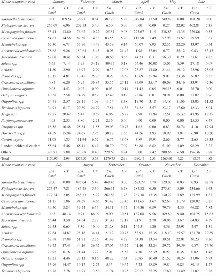
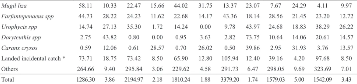
To the extent that the level of detail increased, more biased and less precise the estimates have become. This can be seen in Table 7 where monthly estimated catches by ish categories over 2011 and the associated CV are shown.
Table 5. Results of the Sampling Plan 1 (SP1) – the lowest square root of the mean squared error (RMSE) – by month
for São Paulo coast over 2011. Catches are expressed in tons; CV - coeicient of variation within each month; % B – Bias
expressed as percentage of catch 2011.
Month Catch 2011 Estimated catch CV % B
January 1216.95 1170.96 2.99 -3.78
February 1332.73 1355.35 5.69 1.70
March 1208.75 1279.73 2.91 5.87
April 1299.85 1390.45 2.53 6.97
May 1217.87 1265.60 4.25 3.92
June 1547.84 1498.77 1.88 -3.17
July 1300.29 1286.30 3.86 -1.08
August 2233.64 2194.97 2.18 -1.73
September 1830.74 1810.24 1.88 -1.12
October 3414.64 3379.20 1.74 -1.04
November 1700.62 1579.03 5.00 -7.15
December 1657.89 1542.09 3.43 -6.98
Total 19961.80 19752.69 2.07 -1.05
for example, observed for estimated catch of Cynoscion
jamaicensis in May (Table 7). In Figure 3, monthly
estimated catches for four of the 20 main ish categories landed in São Paulo State are presented, each displaying a diferent situation: estimates with some variability and bias (Micropogonias furnieri), estimates with relatively
large bias (M. atricauda), accurate estimates (O. oglinum),
and estimates with very large variability and bias (C.
brasiliana).
In order to collect data from all 83137 landings carried out in 133 ports on the São Paulo coast over 2011 (census) 32 ield agents, ive monitors and four typists would be required. The scenarios SP1 (lowest RMSE) and SP2 (lowest isheries monitoring cost) were compared to the census methodology and, in both, 77 ports were sampled, reducing the number of monitored ports by 42.1% compared to the census methodology. With this reduction, the same ive monitors and three typists would be required. Considering only SP1, 27 ield agents would be required since a 35.4% reduction in number of monitored landings were observed, decreasing the isheries monitoring costs by 11.2%. To monitor the ports of SP2, 24 ield agents would be required with a 41.5% reduction in number of monitored landings and a 15.4% decrease in isheries monitoring costs.
DISCUSSION
The ishing activity, especially the small-scale ishery, represents a seasonal, diversiied and dynamic activity (CADIMA et al., 2005; ISAAC et al., 2008; MENDONÇA;
MIRANDA, 2008). These characteristics along with the need for accurate information lead to the adoption of complex survey plans for isheries monitoring, such as the sampling methodology for isheries monitoring proposed by IBGE (LIMA-GREEN; MOREIRA, 2012).
The accuracy of the total landed catch estimated through this methodology could only be judged because the true (population) values of landed catch in all municipalities of the São Paulo State are known. Therefore, a sampling distribution could be obtained by applying the same sampling procedure repeatedly (COCHRAN, 1977). The results demonstrated that the mean landed catch is a good estimator of the total landed catch for most municipalities since it was unbiased and had high precision. The low coverage of CI95 was attributed to the non-conformity of the Gaussian distribution used to build these intervals. The small number of possible sets of sampled ports (conglomerates) compromises the use of IC95 to evaluate the precision and the reliability of the estimates (BUSSAB; MORETTIN, 2012).
Table 6. Results of the Sampling Plan 1 (SP1) – the lowest square root of the mean squared error (RMSE) – by ish category
for São Paulo coast over 2011. Catches are expressed in tons; CV - coeicient of variation within each ish category; % B –
Bias expressed as percentage of catch 2011. Landed catch per unit of efort (LPUE) expressed in ton*trip-1.
Minor taxonomic rank Catch 2011
Estimated
catch CV % B
Number of trips
2011
Estimated number of
trips
CV % B LPUE 2011
Estimated LPUE Sardinella brasilienses 4105.09 4150.42 3.38 1.10 205 211 7.52 2.93 20.025 19.670 Xiphopenaeus kroyeri 2759.11 2399.59 5.31 -13.03 17618 14608 18.25 -17.08 0.157 0.164 Micropogonias furnieri 2102.17 2183.93 6.12 3.89 11311 10184 5.17 -9.96 0.186 0.214 Cynoscion jamaicensis 1036.34 1060.41 7.62 2.32 1003 1015 4.26 1.20 1.033 1.045 Macrodon atricauda 705.18 634.20 2.15 -10.07 8277 6136 7.74 -25.87 0.085 0.103 Menticirrhus spp 646.99 674.74 6.98 4.29 3357 3342 3.23 -0.45 0.193 0.202 Anchoviella lepidentostole 612.01 669.00 6.29 9.31 11630 11709 13.52 0.68 0.053 0.057 Selene spp 480.40 482.36 2.44 0.41 849 759 19.24 -10.60 0.566 0.636
Ariidae 454.35 475.63 16.44 4.68 10835 10083 14.49 -6.94 0.042 0.047
Octopus vulgaris 355.26 316.69 3.66 -10.85 722 668 4.22 -7.48 0.492 0.474 Prionotus spp 352.43 375.29 10.78 6.49 600 644 8.08 7.33 0.587 0.583 Opisthonema oglinum 343.43 342.78 0.40 -0.19 888 753 9.31 -15.20 0.387 0.455 Mugil liza 319.68 237.95 14.89 -25.57 7053 6432 12.36 -8.80 0.045 0.037 Oligoplites spp 290.77 285.05 3.16 -1.97 3110 2802 5.70 -9.90 0.093 0.102 Doryteuthis spp 256.73 208.11 4.34 -18.94 2546 2422 3.46 -4.87 0.101 0.086 Trichiurus lepturus 255.64 271.10 9.03 6.05 3865 4144 6.01 7.22 0.066 0.065 Farfantepenaeus spp 249.70 227.30 14.89 -8.97 872 848 4.59 -2.75 0.286 0.268 Urophycis spp 193.85 217.03 13.63 11.96 259 267 6.62 3.09 0.748 0.813 Crassostrea brasiliana 173.82 355.81 34.24 104.70 5354 10591 43.82 97.81 0.032 0.034 Caranx crysos 170.84 158.05 5.39 -7.48 744 787 24.76 5.78 0.230 0.201
Landed incidental catch * 882.45 834.60 6.88 -5.42 10661 8733 2.10 -18.08 0.083 0.096 Others 3215.56 3192.65 4.63 -0.71 39721 37467 9.06 -5.67 0.081 0.085 Total 19961.80 19752.69 2.07 -1.05 83137 80202 7.21 -3.53 0.240 0.246
* Fish of small size and/or low or no commercial value, however landed and marketed, composing the category called “Mistura” in isheries statistics of the São Paulo State.
Figure 2. Order of importance in terms of catches of the 20 main species landed over 2011 on the São Paulo coast. Abscissa with true order for 2011 and ordinate with estimated order; matches between is a point on grey line.
of the sample. Thus, since there is no marked diference in costs between SP1 and SP2, SP1 was chosen as the most appropriate allocation.
Table 7. Results of the Sampling Plan 1 (SP1) – the lowest square root of the mean squared error (RMSE) – by month and
ish category for São Paulo coast over 2011. Catches are expressed in tons; CV - coeicient of variation within each month and ish category.
Minor taxonomic rank January February March April May June Est.
Catch
CV Est. Catch
CV Est. Catch
CV Est. Catch
CV Est. Catch
CV Est. Catch
CV
Sardinella brasilienses 0.00 109.54 36.91 0.61 387.29 5.79 349.84 17.50 249.82 0.00 108.28 0.00 Xiphopenaeus kroyeri 265.09 6.96 202.53 5.40 6.50 0.00 0.00 0.00 0.27 22.92 402.81 7.35 Micropogonias furnieri 55.44 13.80 76.62 10.22 125.51 9.08 223.67 3.15 238.83 13.35 229.86 0.53 Cynoscion jamaicensis 54.61 14.56 82.58 14.88 83.55 5.70 115.58 7.49 52.98 33.52 89.59 3.87 Menticirrhus spp 62.30 6.71 55.96 14.49 43.59 9.14 60.07 8.95 32.55 22.20 33.97 0.54 Anchoviella lepidentostole 78.68 9.26 150.63 15.43 10.05 21.42 1.98 37.04 0.77 55.12 0.83 53.43 Macrodon atricauda 52.08 10.41 60.54 1.06 30.68 0.65 44.23 0.31 56.30 0.29 51.61 4.82 Selene spp 6.65 7.14 3.95 34.19 109.37 0.18 54.46 30.08 15.03 8.59 27.18 0.07 Ariidae 11.80 2.90 16.97 12.99 10.33 17.08 23.27 13.80 21.44 19.12 23.96 25.05 Prionotus spp 13.15 4.81 13.45 25.76 10.97 18.56 16.69 25.94 9.07 23.36 36.07 6.55 Crassostrea brasiliana 0.81 6.20 6.95 36.34 35.55 27.12 37.09 35.17 40.09 34.16 33.91 47.36 Opisthonema oglinum 0.03 4.53 0.02 0.00 0.03 10.14 61.42 0.05 195.15 0.01 26.70 0.00 Octopus vulgaris 10.58 2.58 24.79 0.52 32.49 0.19 23.86 0.01 20.91 0.00 27.07 8.96 Oligoplites spp 54.71 2.57 28.11 1.09 11.54 8.38 19.70 3.18 14.48 11.06 13.03 11.52 Trichiurus lepturus 34.91 6.17 29.89 24.79 17.51 14.33 34.22 5.57 23.17 17.60 18.33 5.04 Mugil liza 12.27 20.62 5.43 19.59 6.06 16.77 7.98 17.94 12.51 15.32 43.95 19.35 Farfantepenaeus spp 4.05 2.35 8.80 12.21 2.36 0.00 0.00 0.00 0.00 0.00 25.35 8.47 Urophycis spp 18.58 16.48 25.84 11.85 29.03 30.73 1.62 0.00 0.83 58.74 4.10 17.94 Doryteuthis spp 44.59 15.94 24.67 2.95 30.12 1.65 44.26 3.93 18.99 3.81 6.90 10.20 Caranx crysos 11.08 1.85 111.94 6.62 16.75 18.68 3.89 19.91 2.66 3.77 2.63 23.33
Landed incidental catch * 55.64 5.46 68.11 8.49 50.79 7.09 56.88 6.82 51.09 3.09 96.29 3.27 Others 323.91 5.88 320.68 8.40 229.68 8.24 0.00 5.42 208.66 6.50 196.36 3.88 Total 1170.96 2.99 1355.35 5.69 1279.73 2.91 1390.45 2.53 1265.60 4.25 1498.77 1.88
Minor taxonomic rank July August September October November December Est.
Catch
CV Est. Catch
CV Est. Catch
CV Est. Catch
CV Est. Catch
CV Est. Catch
CV
Mugil liza 58.11 10.33 22.47 15.66 44.02 31.75 13.37 23.07 7.67 24.29 4.11 9.97 Farfantepenaeus spp 44.73 28.22 24.23 11.62 22.68 14.17 43.36 18.14 28.56 21.45 23.20 12.72 Urophycis spp 14.74 27.13 35.30 1.72 14.24 0.00 9.78 43.97 24.68 18.83 38.29 26.22 Doryteuthis spp 2.75 43.82 0.80 0.00 0.95 3.63 2.82 73.75 10.64 14.06 20.61 14.57 Caranx crysos 0.59 12.06 0.61 28.57 0.70 26.02 0.50 39.86 2.95 31.93 3.76 13.57
Landed incidental catch * 73.71 18.75 73.42 8.50 65.90 12.80 105.94 12.40 39.16 4.20 97.68 8.50 Others 264.66 9.40 295.84 3.06 229.62 4.58 291.73 6.47 298.05 9.69 323.69 7.01 Total 1286.30 3.86 2194.97 2.18 1810.24 1.88 3379.20 1.74 1579.03 5.00 1542.09 3.43
Figure 3. True total landed catches of 2011 (open circle), estimated total landed catches (line), both in tons, and conidence interval of 95% (shaded area) by month to four of the 20 main species landed over 2011 on the São Paulo coast.
of the São Paulo coast with sampling design compared to the census (10.9% in SP1 and 13.8% in SP2).
The more detail is needed and the more variables are involved, the less accurate the estimates become. According to BOLFARINE and BUSSAB (2005), accurate estimates result from considering them explicitly when developing the sampling design, as it is the case herein for the estimated total catch by municipality. Although the variable month has not been considered in the sampling design, estimated monthly total catch for São Paulo State was also a good result since there was suicient information by month in the sample. In contrast, after breaking down these data by ish category, a much lower accuracy was obtained, particularly for some ish categories such as C.
brasiliana, M. Lisa, Farfantepenaeus spp and Doryteuthis
spp, all of them economically important for the São Paulo State. Detailing data even further, by ishing gear or leet type, would only make matters worse.
However, the landed catch per landing (LPUE) turned out to be a robust estimate, for most but a very few ish categories. This was facilitated because all landings of the sampled ports were considered. Furthermore, when
both the catch and the number of trips are simultaneously under- or overestimated, this bias tends to be canceled out. However, since this estimated LPUE was based on a sampling plan designed speciically for the São Paulo State, its performance with the consolidated ishery data from other States with diferent sample designs must be further investigated. The assessment and interpretation of a temporal series of the estimated LPUE may also be a problem, mainly for species with little information in the sample or with less precise estimates, when sample errors are greater than the variations of the LPUE itself.
The results obtained for four ish categories have been selected to illustrate distinct situations that can also occur in other survey samplings for isheries monitoring. First of them is the Opisthonema oglinum, which had very
precise and unbiased estimates since the vast majority of the landings and of the landed catch occurred in ports that had been allocated into the census strata. The second situation is described by the estimated monthly catch of
M. furnieri, which was unbiased but less precise. Many
landings covering a wide range of landed catches of this species occurred in most of the sampled ports, which truly represents the situation in the ports of São Paulo. The third situation is described by M. atricauda, for which the
sampled ports recorded fewer landings and lower catches in comparison to what really happens in all ports. Thus, moderately imprecise and underestimated landed catches were obtained. Finally, C. brasiliana represents the worst
In general, information gathered from well-designed survey samples may have some advantages compared to a complete data collection (census). According to COCHRAN (1977), accurate and reliable estimates can be produced at a much lower cost and data can be obtained and consolidated more quickly applying sampling methods. In addition, survey samplings may have more scope and suppleness regarding the type and amount of information that can be obtained, since only a part of the population is being considered (FAO, 1999). However, these announced advantages were not clearly observed by the sampling design that was applied to monitor the isheries on the São Paulo coast.
Some issues that may cause concern will be mentioned next. The high-diversiied ishing activity afected the accuracy in the estimated catch by ish category. The cost reduction obtained with the sampling was minor and may not compensate the loss of quality of the ishing information compared to the census data. Fishing vessels and ishermen who are not included in the sample cannot be supplied with a proof of activity and of isheries production, documents required to obtain beneits such as bank loans and ishing licenses. The true ishing area covered by the leet in operation might be underestimated, since vessels distribution is underrepresented. Finally, the lack of ishing efort measurements that are more appropriate for each ishing leet makes the ish stock assessment diicult.
The choice of a ishing data collection methodology depends very much on the goals of isheries monitoring (FAO, 1999). In this study, it was clear that a survey sampling for isheries monitoring is very useful when inancial resources are limited and there is the interest only in a broad picture, without details about the catches. It is understood that it is possible to have more detailed and reliable ishing data increasing the complexity of the sampling design and the costs of the ishing monitoring as well. Or even, to begin with a simple sampling design and, as far as it is feasible, gradually expand to a census methodology (FAO, 1999). In this case, low cost strategies, such as self-registration and mobile ield agents, may be adopted. Both strategies have been adopted since the beginning of the Fishing Activity Monitoring Program (PMAP) of the São Paulo coast. However, regardless of the methodology and whatever the cost of a isheries monitoring program might be, one thing is for sure, it will always be lower than the economic, social and
environmental costs of not having quality data to perform evidence based isheries management.
ACKNOWLEDGEMENTS
This work is part of the doctoral degree in Biological Oceanography of the irst author working under the supervision of the second. We express our thanks to the isheries scientists and technical team of the Fishing Activity Monitoring Program (PMAP) and to the Fisheries Institute of the Department of Agriculture and Food Supply of São Paulo State. We are also thankful to MSc Aristides Pereira Lima Green (IBGE) for all his contribution.
REFERENCES
ARAGÃO, J. A. N.; MARTINS, S. Censo Estrutural da Pesca, Coleta de Dados e Estimação de Desembarques de Pescado. Brasília: IBAMA, 2006. 180 p.
ÁVILA-DA-SILVA, A. O.; CARNEIRO, M. H.; FAGUNDES, L. Sistema gerenciador de banco de dados de controle estatístico de produção pesqueira marinha – ProPesq. In: Anais do XI Congresso Brasileiro de Engenharia de Pesca e I Congresso Latinoamericano de Engenharia de Pesca. Recife, 1999. p. 824-832.
ÁVILA-DA-SILVA, A. O.; CARNEIRO, M. H.; MENDONÇA, J. T.; BASTOS, G. C. C.; MIRANDA, L. V.; RIBEIRO, W. R.; SANTOS, S. Produção Pesqueira Marinha e Estuarina do Estado de São Paulo - Dezembro de 2014. Inf. Pesq. São Pau-lo, v. 54, p. 1-4, 2015.
BOLFARINE, H.; BUSSAB, W.O. Elementos de Amostragem. 1.ed. São Paulo: Edgar Blücher, 2005. 274 p.
BUSSAB, W. O.; MORETTIN, P. A. Estatística Básica. 7.ed. São Paulo: Saraiva, 2012. 540 p.
CADDY, J. F.; BAZIGOS, J. P. Practical guidelines for statistical monitoring of isheries in manpower limited situations. FAO Fisheries Technical Paper.nº. 257. Rome: FAO, 1985. 86 p. CADIMA, E. L. Fish stock assessment manual. FAO Fisheries
Technical Paper. nº. 393. Rome: FAO, 2003. 161 p.
CADIMA, E. L.; CARAMELO, A. M.; AFONSO-DIAS, M.; CONTE DE BARROS, P.; TANDSTAD, M. O.; DE LEIVA--MORENO, J. I. Sampling methods applied to isheries scien-ce: a manual. FAO Fisheries Technical Paper. nº 434. Rome: FAO, 2005. 88 p.
COCHRAN, W. G. Sampling Techniques. New York: John Wiley & Sons, 1977. 428 p.
DIAS-NETO, J. Pesca no Brasil e seus aspectos institucionais - um registro para o futuro. Rev. CEPSUL - Biodivers. Con-serv. Mar., v. 1, n. 1, p. 66-80, 2010.
DIAS-NETO, J. Números e Baionetas – A Nova Estatística da Produção Pesqueira do Brasil. Erro Estatístico ou Equívoco Político? Pesca & Mar - Informativo SAPERJ (março/abril). Rio de Janeiro/RJ. v. 132, p. 31-34, 2011.
HILBORN, R.; WALTERS, C. J. Quantitative isheries stock as-sessment: choice, dynamics and uncertainty. New York: Cha-pman and Hall, 1992. 570 p.
HORVITZ, D. G.; THOMPSON, D. J. A generalization of sam-pling without replacement from a inite universe. J. Am. Stat. Assoc., v. 47, n. 260, p. 663-685, 1952.
ISSAC, V. J.; RUFFINO, M. L.; MELLO, P. Considerações sobre o Método de Amostragem para a Coleta de Dados sobre Cap-tura e Esforço Pesqueiro no Médio Amazonas. In: IBAMA. (Org.). Recursos Pesqueiros do Médio Amazonas: Biologia e Estatística Pesqueira. Brasília: Edições IBAMA, 2000. p. 175-199.
ISSAC, V. J.; ESPÍRITO SANTO, R. V.; NUNES, J. L. G. A es-tatística pesqueira no litoral do Pará: resultados divergentes. Pan-Am. J. Aquat. Sci., v. 3, n. 3, p. 205-213, 2008. LIMA-GREEN, A. P.; MOREIRA, G. G. Metodologia Estatística
da Pesca: pesca embarcada.Textos para Discussão. Diretoria de Pesquisas. Rio de Janeiro: IBGE, 2012. p. 1-52.
LUMLEY, T. Complex surveys: a guide to analysis using R. Ho-boken: John Wiley & Sons, 2010. 276 p.
LUMLEY, T. Survey: analysis of complex survey samples. R pa-ckage version 3.30. 2014.
MENDONÇA, J. T.; MIRANDA, L. V. Estatística pesqueira do litoral sul do estado de São Paulo: subsídios para gestão compartilhada. Pan-Am. J. Aquat. Sci., v. 3, n. 3, p. 152-173, 2008.
R CORE TEAM R. A language and environment for statistical computing. R Foundation for Statistical Computing. Vienna, Austria. 2015. Disponível em: <http://www.R-project.org>. Acesso em: 10 dez. 2015.