Competing Spin Dynamics in Ising Systems
W. Figueiredoand B.C.S. Grandi
Departamento de Fsica, Universidade Federal de Santa Catarina 88040-900, Florianopolis, SC, Brazil
[email protected] Received 15 October 1999
We study ferromagnetic and antiferromagnetic Ising models in contact with a heat reservoir, and subject to an external source of energy. The contact with the heat bath is simulated by a single-spin ip Glauber dynamics, while the ux of energy is simulated by the two-spin exchange Kawasaki process. Pair approximation and Monte Carlo calculations are employed to determine the phase diagram for the stationary states of the model. We report the results we have obtained in one, two and three dimensions. For instance, in one dimension, while the pair approximation predicts a phase transition for the ferromagnetic case, this is not corroborated by the Monte Carlo simulations. We also use Monte Carlo simulations to evaluate the static and dynamic critical exponents at the transition lines between nonequilibrium steady states. We show that the critical exponents agree with those of the corresponding equilibrium Ising model, for which detailed balance is obeyed.
I Introduction
The study of thermodynamic properties of nonequilib-rium systems is a challenging subject because there is still no complete theory to account for these phenom-ena. That is, formalisms like that of equilibrium ther-modynamics, or based on the ensembles of equilibrium statistical mechanics, are still lacking. The behavior of systems out of equilibrium may appear quite complex; many interesting models have been studied. We refer to the books of Marro and Dickman [1] and Privman [2] for a survey in several interacting particle systems on a lattice. For a deeper insight into mathematical questions, and development of the formalism related to phase transitions of interacting particle systems, the books of Ligget [3] and Konno [4] are of fundamental importance. Kinetic Ising models on the lattice are very often used to describe the time evolution and the cor-responding steady states of a great variety of interact-ing particle systems, as for example catalysis, contact process, domain growth, phase separation, and trans-port phenomena. Aside from a few approximate ana-lytical methods used to investigate these systems, com-putational methods have been the main tool to study nonequilibrium steady states. In this work we report some studies on kinetic Ising spin systems where the dynamics is dictated by competing stochastic process. Each of the dynamical process we consider saties de-tailed balance, which drives the system towards equi-librium states. An interesting situation appears when
re-sult conrmed a previous pair-approximation calcula-tion by Dickman [8] on the same model. In his mean eld pair-approximation treatment, he found the value q = 0:72 for the tricritical point. Models of combined Glauber and Kawasaki dynamics were investigated pre-viously by DeMasi et al. [9, 10] for the particular case of an innitely large value of the Kawasaki transition rate. In this limit, the fast exchange of spins leads to a reaction-diusion equation for the local magnetization at innite temperature.
If the two-spin exchange depends on the spin cong-uration, a new behavior emerges from the competition between Glauber and Kawasaki dynamics: a ferromag-netic Ising system, depending on the value of the com-petition parameter, can exhibit three dierent types of magnetic ordering: a ferromagnetic, paramagnetic or antiferromagnetic, as was shown by Tome and de Oliveira [11]. In their model, the Glauber process sim-ulates the contact with a heat bath at a xed tem-perature, and the two-spin Kawasaki exchange simu-lates a continuous ux of energy into the system. They show that, as the ux of energy is increased, the sys-tem goes continuously from the ferromagnetic to the paramagnetic state, and, for a further increase in the energy ux, it goes continuously to an antiferromag-netic stable state. They employed a dynamical pair approximation in their calculations in two dimensions; the results show that the model can be seen as a ki-netic Ising model where ferromagki-netic Glauber dynam-ics at a given temperature competes with an antifer-romagnetic Kawasaki dynamics at zero temperature. This model is not symmetric to the antiferromagnetic Ising case: by employing the same competitive dy-namics for the two-dimensional antiferromagnetic Ising model, the pair approximation gives only a transition line between the antiferromagnetic and paramagnetic phases at low ux of energy [12]. If we increase the energy ux, the only stable states we nd are of the paramagnetic type. The ferro- and antiferromagnetic two-dimensional Ising models with competing Glauber and Kawasaki dynamics were also studied by Monte Carlo simulations [13, 14]. The phase diagrams and the corresponding stationary critical exponents were deter-mined. The values found for the critical exponents sup-port the idea that equilibrium and nonequilibrium Ising models, which both exhibit up-down symmetry, belong to the same universality class [15]. For the particular case where the Glauber and Kawasaki dynamics com-pete at T = 0, in the antiferromagnetic Ising model, the pair approximation predicts ferro, para and anti-ferromagnetic phases as the strength of the exchange between two nearest neighbor spins in the Kawasaki dynamics changes [16]. Using a quantum formulation
of the master equation, Artz and Trimper [17] studied the kinetic Ising model with long-range interactions, subject to competing Glauber and Kawasaki dynamics. They showed that in the exchange-dominated case the system is strongly correlated for each value of temper-ature.
In Section II we establish the equations of motion for the kinetic Ising model with Glauber and Kawasaki competitive dynamics, and show some results obtained within the dynamical pair approximation. In Section III we present the corresponding results from Monte Carlo simulations, and in Section IV we present our conclusions.
II Equations of motion and the
dynamical pair
approxima-tion
We consider an Ising model on a hypercubic lattice with N sites. The energy of the system in the state = (
1 ;
2 ;:::;
N), where the spin variable assumes the values
i=
1, is given by E() =,J
X (i;j) i j ; (1)
where the summationis only over spins that are nearest neighbors on the lattice, and the casesJ >0, ferromag-netic, and J < 0, antiferromagnetic, are considered. LetP(;t) be the probability of nding the system in state at time t. The evolution of P(;t) is given by the following master equation :
dP(;t) dt
=X
0
[P( 0
;t)W( 0
;),P(;t)W(; 0)]
; (2) whereW(
0
;) gives the probability, per unit time, for the transition from the state
0 to state
. In order to take into account the two competing processes, we assume that
W( 0
;) =pW G(
0
;) + (1,p)W K(
0
;): (3) In this equation,
WK(0;) = X (i;j)
0 1;
1 0 2;
2::: 0 i;
j::: :::0
j; i:::
0 N;
Nwij() (5) is the two-spin exchange Kawasaki process, which mim-ics the ux of energy into the system. In the above sum-mation, only nearest-neighbor pairs of spins are consid-ered.
In these equations, wi() is the transition
proba-bility, per unit time, of ipping spin i, while wij() is
the transition probability, per unit time, of exchanging nearest-neighbor spins i and j. We use the following prescriptions for wi() and wij():
wi() = min
1; exp(, Ei
kBT )
; (6)
which is the Metropolis transition rate [18], and wij() =
0; for Eij0
1; for Eij> 0 ; (7)
where Eiis the change in energy when spin i is ipped
and Eij is the change in energy after exchanging the
nearest neighbor spins i and j.
From Eq. (2) it is easy to derive expressions for the evolution of the magnetization,hii, and for the corre-lation function between nearest-neighbor spins,hjki. They are given by
dhii
dt = pAi+ (1,p)Bi; (8) dhjki
dt = pAjk+ (1,p)Bjk; (9) where
Ai = ,h2iwi()i; (10)
Ajk = ,h2jkwj()i,h2jkwk()i; (11)
Bi = X
l (NN of i)
h(l,i)wlii; (12)
Bjk = X
l6=k (NN of j)
h(lk,jk)wjl()i+ X
l6=j (NN of k)
h(jl,jk)wkl()i; (13) where by (NN of i) we denote a summation over the nearest neighbors of site i.
Although Eqs. (8) - (13) are exact, the mean values of the right-hand sides of these equations cannot be cal-culated, because we do not know the exact expression
for the probability P(;t). Thus we need to consider an approximate expression for P(;t). We employ the pair approximation [19] to evaluate the mean values on the right hand sides of Eqs. (10) - (13). We rst di-vide our lattice into two interpenetrating sublattices, and look for solutions such thathii= m
1for any spin i belonging to sublattice 1, andhji= m
2 for any spin j belonging to sublattice 2. The correlation function for any pair of nearest-neighbor spins i and j is written as hiji = r. If we then perform these calculations employing the pair approximation, we easily obtain ex-pressions for the time evolution of m1, m2and r. These expressions are very lengthy, and can be found, for the ferromagnetic case, in the work of Tomeand de Oliveira [11].
We look for stationary solutions of Eqs. (8) and (9) characterized by constant values of m1, m2 and r. We expect three dierent solutions: m1 =
,m 2
6
= 0 (antiferromagnetic stable states), m1 = m2
6
= 0 (ferro-magnetic stable states), and m1 = m2 = 0 (paramag-netic stable states). The equation dh
1 2i
dt = drdt = 0 ,
with m1 = m2 = 0, gives the paramagnetic stationary states. If we write the order parameter for the fer-romagnetic phase in the form mF = m1
+m 2
2 , and for the antiferromagnetic phase as mA = m1,m
2
2 , we can expand the right-hand side of Eq. (8) for i = 1 and 2. Retaining only terms linear in mF and mA, we can
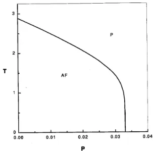
Figure 1. Phase diagram of the two-dimensional ferromag-netic Ising model with competing dynamics in the pair ap-proximation. T is the temperature, in units of
J k
B, and P =
1,p
p measures the competition between the Kawasaki and Glauber dynamics. F,P andAF denote the ferromag-netic, paramagnetic and antiferromagnetic phases, respec-tively. A,BandC represent selected steady states. evolution towards the stationary stateB, absorbing en-ergy from the electromagnetic beam, in such a way that, locally, this favors an antiferromagnetic alignment of the spins. Despite absorbing energy from the beam, in-creasing the antiferromagnetic correlation, the station-ary stateBis still a globallyparamagnetic state. When, nally, the system arrives in the stationary stateB, the system becomes transparent to the electromagnetic ra-diation of the beam (indeed, there occur small energy uctuations, the energy of the system sometimes in-creasing due the absorption, at other times dein-creasing due to the presence of the heat bath). If, for instance, the incident beam is switched o when the system is in steady state B, it will return to the initial stateA, by giving up energy to the heat bath; therefore the para-magnetic states A and B are dierent, because at the steady state B, the antiferromagnetic correlations are higher than in the equilibrium state A. This higher antiferromagnetic correlation is maintained by the con-stant ux of energy into the system. In order for the system to arrive at steady state C from state B, we must increase the ux of energy, which in our case is equivalent to increasing the parameter q: the system will absorb energy from the beam until it reaches the state C, when will again become transparent to the radiation beam, although the antiferromagnetic corre-lation and energy are now higher than in state B. For an extremely high ux of energy, that is,qalmost equal to 1, the system will reach a fully antiferromagnetic or-dered state for whatever value of the heat bath temper-ature. That is, the correlations induced by the single
spin-ip Glauber transitions are immediately destroyed by the interaction of the system with the radiation beam, which returns it to its highest possible energy state per spin, E = 2J. Thus, for a given stationary state, characterized by the parametersTandq, the uc-tuation of the energy is due interactions with the heat bath and with the electromagnetic radiation. There-fore, in its steady states, the system becomes trans-parent to the radiation: antiferromagnetic correlations are created (due the ux of radiation) and destroyed (due the one-spin-ip Glauber transitions). If p = 1, the stationary states are the equilibrium ones, and the critical temperature is given byk
B T
c = 2
:885J, which is the equilibrium critical temperature in the Bethe-Peierls approximation.
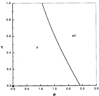
We present in Fig. 2 the phase diagram of the competing model for antiferromagnetic coupling. This phase diagram was obtained using the dynamical pair approximation to solve the coupled system of equations on the square lattice. It is interesting to note that the stable antiferromagnetic region is very small compared with the ferromagnetic case shown in Fig. 1. The an-tiferromagnetic phase is destroyed by a small input of energy. The paramagnetic-ferromagnetic transition line is absent in this antiferromagnetic model. As expected, the ux of energy into the system breaks the symmetry between the ferromagnetic and antiferromagnetic Ising models observed in equilibrium.
Figure 2. Phase diagram of the kinetic antiferromagnetic Ising model in two dimensions. T is the heat-bath temper-ature and P =
1,p
p is related to the ux of energy. The system exhibits only the antiferromagnetic (AF) and para-magnetic (P) phases, separated by a line of continuous non-equilibrium transitions.
with competing Glauber and Kawasaki dynamics [24]. In this pair approximation calculation, we see that the phase diagram exhibits a continuous phase transition between the paramagnetic and the antiferromagnetic phases for the nonequilibrium case (p 6= 1). As is to be expected, for p = 1, the pair-approximation gives no phase transition at nite temperature for the Ising model. The ferromagnetic ordered state appears only at zero temperature. Similar calculations performed for the one-dimensional antiferromagnetic Ising model show that for any value ofp, andT6= 0, the only phase that remains is the paramagnetic one. Although this one-dimensional nonequilibrium Ising model has no ex-act solution, our Monte Carlo simulationsfor this model clearly show that the transition line of Fig. 3 is absent. The phase transition observed in this gure is indeed an artifact of the pair approximation. This approximation underestimates uctuations and can give wrong results when applied to nonequilibrium one-dimensional situa-tions.
Figure 3. Nonequilibrium phase diagram of the one-dimensional ferromagnetic Ising model, as obtained in the pair approximation. Here = exp(
,4J k
B T) and
P = 1,p
p is related to the energy ux. The stationary states of the system are represented by the paramagnetic (P) and antifer-romagnetic (AF) phases, separated by a line of continuous nonequilibrium transitions. The singular point P = 0 and = 0 corresponds to the fully ordered ferromagnetic state.
III Monte Carlo simulations
As we have just seen, Monte Carlo simulations of the nonequilibrium one-dimensional Ising model gave re-sults completely dierent from the predictions of the pair approximation. In this section, therefore, we
present phase diagrams of the ferro- and antiferromag-netic Ising model in two dimensions, obtained by Monte Carlo simulations, in order to compare them with those of Figs. 1 and 2. We also calculated the static and dynamic critical exponents at the steady state phase transitions, and extended the simulations to the three-dimensional version of the competing model we are con-sidering.
Let us rst consider the square lattice. We take lat-tices withLL=N sites, with L ranging fromL= 6 up toL= 80. We used periodic boundary conditions in all of our simulations. We started the simulations with dierent initial states, in order to guarantee that the -nal stationary states we use in our calculations are the correct ones. For a given temperature T, and a chosen value of the probabilityp, we choose at random a spin i, from a given initial conguration. We then generate a random number
1 between zero and unity. If
1 p we perform the Glauber process; in this process, we calculate the value ofw
i(
). We generate another ran-dom number
2: if
2
w
i(
), we ip spini, otherwise we do not. If
1
> p we perform the Kawasaki pro-cess. We generate another random number
3 in order to select one of the four nearest neighbors of spini, say j. Then we nd w
ij, and exchange the selected spins only if w
ij = 1. We note that the stationary regime is established after 104
N Monte Carlo steps, for all lattice sizes considered. One Monte Carlo step equals N spin-ip or exchange trials. In order to estimate the quantities of interest, we used 510
4Monte Carlo steps to calculate averages.
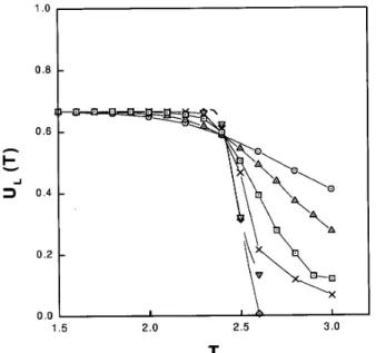
In order to locate the critical temperature for each value of p, we plotted the reduced fourth-order cumu-lant [25] U
L(
T) (see Eq.(16) below) as a function of temperature T, for several values of L. Since this value is independent of lattice size at the critical temperature T
c, the crossing point of these curves gives T
c [26]. In Fig. 4 we exhibit the reduced fourth-order cumulant for p= 0:5. From this gure we estimateT
c= 2
:420:01in units of J
kB. We have also considered other values of pin our analysis, in order to determine the complete phase diagram of the model. The resulting phase diagram can be seen in Fig. 5, where we plot =exp(,
J k
with the Kawasaki process was independent of the spin congurations, here we do not observe any dynamic tri-critical behavior. On the other hand, the tri-critical tem-perature exhibits a slight maximum near p = 0:3. For p < 0:3, where the Kawasaki process is the dominant one, the critical temperature approaches zero as p!0. For the pure Kawasaki case, p = 0, the evolution of the system is the same for whatever temperature, that is, we always go to the state of maximum energy compat-ible with a given initial magnetization. For instance, if the initial state is a paramagnetic one, the nal state will be the one where the staggered magnetization per spin reaches its maximum value, that is, 1.
Figure 4. Reduced fourth-order cumulant UL(T), for p = 0:5, as a function of temperatureTfor several lattice sizesL. Circles correspond toL= 6, triangles toL= 10, squares to L= 20, crosses to L= 40, downward triangles toL= 60, and diamonds L = 80. We join the data points for each lattice size by a broken line to guide the eye. The critical temperature isT
c= 2
:420:01, in units of J k
B.
By employing nite-size scaling relations [25, 26], we can evaluate the stationary critical exponents as-sociated with these transitions. For a system with LL = N spins, with periodic boundary conditions, we dene, at the stationary states, the \magnetization" per spin ML and the \susceptibility" per spin L as
ML =
hjmji; (14)
L = N
fhm 2
i,hjmji 2
g; (15)
where m = 1 N
P N i=1
i. We also dene the reduced fourth-order cumulant UL as
UL= 1 ,
hm 4
i 3hm
2 i
2: (16)
The above-dened quantities obey the following nite-size scaling relations in the neighborhood of the sta-tionary critical point:
ML(T) = L ,
M
0(L 1
); (17)
L(T) = L
0(L 1
); (18)
UL(T) = U0(L 1
); (19)
where = (T,Tc) Tc , T
c being the critical temperature for each value of p.
Figure 5. Phase diagram of the two-dimensional competing ferromagnetic Ising model. = exp(,
J k
B
T), and (1 ,p) is related to the energy ux. F, P and AF refer to the ferromagnetic, paramagnetic and antiferromagnetic phases, respectively.
Taking the derivative of Eq. (19) with respect to temperature T, we obtain the following scaling relation:
U0
L(T) = L 1 U
0 0(L
1 ) Tc
; (20)
so that U0 L(T
c) = L 1
U 0 0
(0) T
c . We can then nd the critical exponent from the slope of the straight line which is the best t to the data points of U0
L(T
c) for each value of L. Fig. 6 is a log-logplot of U0
L(T
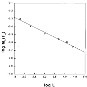
c) versus L, for p = 0:5: from the best t to the data we nd = 1:130:04. In Fig. 7, we exhibit a log-log plot of the magnetization ML(Tc) at the critical temperature, Tc, versus L, for p = 0:5. From the slope of the straight line, which is the best-t to the Monte Carlo data points, and using Eq. (17), we obtain the stationary critical ratio
: our estimate in this case is
= 0:13
0:01. Another sta-tionary critical exponent of interest is that associated with the susceptibility. We can nd the ratio
relation given in Eq. (18). First, we can construct a log-log plot ofL(T) versus L, at the critical tempera-tureTc; then from the slope of the best-t straight line to the data, we obtain, forp= 0:5, = 1:700:05, as can be seen in Fig. 8. We can also estimate the same ratio by a log-log plot of the maximum value of the susceptibility versus L. It is easy to see that if TLmax is the value of T for which L(T) is maximum, then TLmax = Tc+ u
max
L1
, where umax is a constant, inde-pendent ofL, which maximizes
0(
u). Based on these arguments, we immediately see that the maximum of the susceptibility also scales as L. In this way, from Fig. 8, we obtain = 1:650:05 for p= 0:5.
Figure 6. Log-log plot of U 0 L(
Tc) versus L for p = 0:5. The straight line is the best t to the data, which gives = 1:130:04.
Figure 7. Log-log plot of the magnetization ML(Tc) versus L, forp= 0:5. From the slope of the straight line, which is the best t to the data points, we nd
= 0
:130:01.
Figure 8. Log-log plot of the susceptibility L(T) versus L. Circles: L(T) atT =Tc; triangles: L(T) at its max-imum. The straight lines are best ts to the data points. From the slopes we obtain
= 1
:700:05 (circles), and
= 1
:650:05 (triangles).
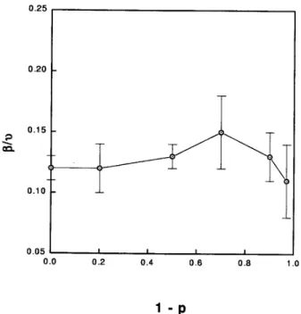
Figure 9. Critical exponentas a function of the parameter (1,p) at the ferromagnetic-paramagnetic transition line of Fig. 5.
and 11 we exhibit our results for and
, respectively, for several values of p. The exact values for the equi-librium Ising model exponents are well known: = 1, = 1=8 and = 7=4. As we can see, our estimated values for
and
, reported in Figs. 10 and 11, are in accord with the corresponding values at equilibrium. We have also calculated the critical exponents at the continuous transition line between the paramagnetic and antiferromagnetic phases. For p = 0:03, for in-stance, we found the following values: T
c= 6
:820:02, = 0:970:05,
= 0
:130:01, and = 1
:830:06.
Figure 10. Ratio
as a function of the parameter (1 ,p) at the ferromagnetic- paramagnetic transition line of Fig. 5.
Figure 11. Ratio
as a function of the parameter (1 ,p) at the ferromagnetic- paramagnetic transition line of Fig. 5.
In Fig. 5, at higher temperatures, we only see a transition between the paramagnetic and the antiferro-magnetic phases. When the Glauber dynamics domi-nates, only paramagnetic stationary states are possible. However, as the internal energy of the system increases, which is equivalent in our description to the predom-inance of the Kawasaki dynamics, long-range antifer-rromagnetic order appears. A detailed Monte Carlo analysis along with nite-size scaling arguments, at in-nite temperature, shows that the transition occurs for p
c = 0
:0730:003, that is, the system is driven al-most exclusively by Kawasaki dynamics [27]. Within the accuracy of our Monte Carlo statistics, the value we found is the same as the one obtained for the isotropic majority-vote model on a square lattice [28]. In this model a spin variable
i =
1 is chosen at random on a square lattice at each discrete time. The chosen spin adopts, with probabilityp, the sign of the major-ity of its four nearest neighboring spins, and the sign of the minority with probability (1,p). As the num-ber of nearest neighbors is even, the chosen spin ips with probability 1=2 when there are equal numbers of positive and negative spins in its neighborhood. The only transitions in the isotropic majority-votemodel are single-spin ips. As was shown by de Oliveira [28], this model can be regarded as composed of two processes: a noiseless zero-temperature process, and an innite-temperature one, where the spins are distributed at random. In this sense, our model shows some resem-blance to the isotropic majority-vote model, where only single-spin ips are considered. The noiseless zero-temperature process in that model is replaced here by a spin-exchange Kawasaki dynamics at an innitesimally negative temperature; on the other hand, the eect of the innite-temperature process in the majority-vote model is equivalent in our case to a Glauber dynamics with a transition rate of 1=2. From the simulationdata, we obtained the critical exponents at the transition line between the paramagnetic and the antiferromagnetic phases, at innite temperature, for this nonequilibrium stochastic Ising spin system. The log-log plot ofU
0 L(
p c) versus L gives = 1:00:1. In addition, the log-log plot of the staggered magnetization,M
L( p
c) versus L, at the critical probabilityp
c, gives us the ratio ; the estimated value obtained from the slope of the best-t straight line to our data is
= 0
:130:01. The station-ary critical exponent associated with the susceptibility can be found by employing two dierent approaches, as was explained before: we can construct a log-log plot of
L(
p) versus L, at p
c; then, from the slope of the straight line, which is the best t to the data points, we obtain the value
= 1
value of the susceptibility versusL. It is easy to see that ifpmaxL is the value ofpfor which L(p) is maximum, thenpmaxL =pc+u
max
L1
, whereumax is a constant, inde-pendent ofL, which maximizes
0(
u). Based on these arguments, we immediately see that the maximum of the susceptibility also scales asL. In this way, we ob-tain = 1:700:01. The values we have found for the stationary critical probabilitypc and for the set of crit-ical exponents are in agreement with those obtained by de Oliveira [28] for the isotropic majority-vote model on the square lattice. As we have pointed out, this fact must be related with the similarities between the competing processes in the two models.
We have also determined the dynamical critical ex-ponentzfor this competing Glauber and Kawasaki dy-namics [30]. Following Suzuki [29], dynamic nite-size scaling theory asserts that the magnetization of a sys-tem of linear size L, at its critical point, evolves in time according to the scaling relation
M(t;L) =L ,
f(L ,z
t): (21)
If we consider very large lattices, it is expected that the magnetization does not depend on the lattice size. Then, it is easy to see thatM(t;L) can be written as
M(t;L) =At ,z
; (22)
where A is a constant that does not depend onL, and the last equation is valid only for large values of L. Then, taking into account the last equation, we can evaluate the exponentz from a log-log plot ofM(t;L) versus t, for a xed lattice size L, once we know
,
given in Fig. 10.
The Monte Carlo method was used again to follow the evolution of the magnetization in time for the com-peting model we are studying. First of all, we select a given value of competition parameterp. For this value of p we read in Fig. 5 its critical temperature, corre-sponding the transition between the ferromagnetic and paramagnetic phases. After initializing the system in its ground state, it evolves in time (measured in Monte Carlo steps); we record the magnetization at intervals of 10 Monte Carlo steps.
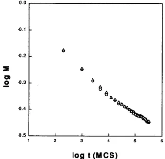
In Fig. 12 we exhibit a log-log plot of M(t) ver-sus t for two lattice sizes, L = 160 and L = 320, for p= 0:5. We see that the decay of M(t) is almost in-dependent of L, which allows us to use Eq. (22) to evaluate the critical exponent z. In these calculations we used 100 and 50 samples for the small and large lattices, respectively. We followed the decay of mag-netization up to 320 Monte Carlo steps. If we discard the rst fty Monte Carlo steps, we can t our data points to a straight line, and we obtain from its slope
the value z = 0:0650:001. We have discarded the initial data points because we want to study the sys-tem in its second regime, where a power-law decay of the magnetization is expected [31]. Taking (from Fig. 10) our result = 0:130:01 for p= 0:5, we estimate z= 2:00:2.
Figure 12. Magnetization as a function of time, measured in Monte Carlo steps (MCS) for p = 0:5. Measurements were made every 10 MCS, between 10 and 320 MCS. Lat-tice sizes: (160160) (small circles) and (320320)(small triangles).
In Fig. 13 we show a plot of the exponent z as a function of (1,p). For all values ofpwe used lattices of size L = 320, and runs of up to 320 Monte Carlo steps. As we can see, the values of the dynamical crit-ical exponent uctuate around z = 2. This indicates that the underlying symmetries of this model are not aected by the energy ux. We would like to point out that since in our simulations the magnitude of our esti-mated errors can be as large as 0.2, the above assump-tion can not be taken as a rigorous statement. But we expect that for whatever value of the energy ux, the critical exponentz must remain the same, because the intensity of the ux of energy cannot change the uni-versality class of this competing model. For the special case ofp= 1, that is, when the system satises detailed balance, we found z = 2:00:1. This value must be compared with the best estimates for this exponent ob-tained through intensive use of large-scale simulations: for instance, Stauer [32] found z = 2:18 for a square lattice with L = 496640 and Linke et al. [33] found z= 2:16 for a square lattice withL= 10
instance, forp= 0:03, we foundz= 2:00:2. In par-ticular, for the transition at innite temperature, where the critical probability is p
c = 0
:073, the value of the dynamical critical exponent zis 1:90:1.
Figure 13. Dynamical critical exponent z as a function of (1,p) at the transition line between ferro and paramag-netic phases. The estimated values of z uctuate around the value 2:0.
ForJ < 0 (antiferromagnetic coupling), the phase diagram for competing Glauber and Kawasaki dynam-ics was also obtained through Monte Carlo simula-tions [14]. The phase diagram is very similar to the one found in the dynamical pair approximation (Fig. 2). At T = 0, for instance, the critical value of p is 0:965 while in the pair approximation its value is 0:968. We also evaluated the critical exponents along the antiferromagnetic-paramagnetic transition line [14]: as for the ferromagnetic case, the critical exponents compare very well with the analogous static exponents of the corresponding two-dimensional equilibrium Ising model.
Finally, we studied the three-dimensional version of the competing Glauber and Kawasaki dynamics for the ferromagnetic Ising model [34]. We used Monte Carlo simulations to nd the phase diagram for the station-ary states and the corresponding critical exponents. The phase diagram is similar to that observed in two-dimensions (Fig. 5). Although the stationary states are mainly ferromagnetic at low temperatures, an anti-ferromagnetic phase appears for extremely high values of the ux of energy. The region of the phase diagram occupied by the antiferromagnetic phase is larger than in the two-dimensional case. For instance, at very high values of temperature the critical value for the param-agnetic to antiferromparam-agnetic transition isp= 0:3, while the value in two dimensions isp= 0:073. At zero tem-perature, we observe only a ferromagnetic steady state, for any value of the competition parameter. We have
also calculated the static critical exponents as a func-tion of the competifunc-tion parameterp. Forp= 0:5, for instance, we nd = 0:670:04,
= 0
:530:01 and
= 1
:930:03. These exponents are almost independent of p. We would like to stress that the values we have obtained for these critical exponents compare very well with the analogous static exponents of the equilibrium three-dimensional Ising model. For instance, numerical investigations of the equilibrium model by Ferrenberg and Landau [35] yield= 0:6289 and
= 0
:518. As this nonequilibrium model preserves up-down symmetry, it is expected that it belongs to the same universality class as the equilibrium Ising model [15].
IV Conclusions
the critical exponents along the antiferro-paramagnetic transition line are those expected for the equilibrium Ising model in two dimensions. We have also studied the three-dimensional version of the competing Glauber and Kawasaki dynamics for the ferromagnetic Ising model. Our simulations gave a phase diagram which is similar to that observed for the two-dimensional fer-romagnetic Ising model. At zero temperature the sta-ble states are of the ferromagnetic type, regardless of the value of the competition parameter; the antiferro-magnetic phase occupies a larger region of the phase diagram than in the two-dimensional case. The static critical exponents were calculated along the transition lines. The values we found are independent of the com-petition parameter, and agree with the static exponents of the equilibrium three-dimensional Ising model. As the Glauber and Kawasaki dynamics preserve the up-down symmetry of the Ising model, even when both operate simultaneously, it is expected that the result-ing nonequilibrium model belongs to the universality class of the equilibrium Ising model.
Acknowledgements
We are very grateful to T^ania Tome and Ron Dick-man for the careful revision of the Dick-manuscript. This work was partially supported by the Brazilian agencies CNPq and FINEP.
References
[1] J. Marro and R. Dickman, Nonequilibrium Phase Tran-sitions in Lattice Models(Cambridge University Press, Cambridge, 1999).
[2] V. Privman, ed., Nonequilibrium Statistical Mechanics in One Dimension(Cambridge University Press, Cam-bridge, 1996).
[3] T. M. Liggett, Interacting Particle Systems (Springer-Verlag, New York, 1985).
[4] N. Konno,Phase Transitions of Interacting Particle Sys-tems(World Scientic, Singapore, 1994).
[5] R. J. Glauber, J. Math. Phys.4, 294 (1963).
[6] K. Kawasaki, in Phase Transitions and Critical Phe-nomena, edited by C. Domb and M. S. Green (Aca-demic, London, 1972), vol. 4.
[7] J. M. Gonzalez-Miranda, P. L. Garrido, J. Marro and J. L. Lebowitz, Phys. Rev. Lett.59, 17 (1987).
[8] R. Dickman, Phys. Lett. A122, 463 (1987).
[9] A. DeMasi, P. A. Ferrari and J. L. Lebowitz, Phys. Rev. Lett.55, 1947 (1985).
[10] A. DeMasi, P. A. Ferrari and J. L. Lebowitz, J. Stat. Phys.44, 589 (1986).
[11] T. Tome and M. J. de Oliveira, Phys. Rev. A40, 6643 (1989).
[12] B. C. S. Grandi and W. Figueiredo, Phys. Rev. B 50, 12595 (1994).
[13] B. C. S. Grandi and W. Figueiredo, Phys. Rev. E 53, 5484 (1996).
[14] B. C. S. Grandi and W. Figueiredo, Phys. Rev. E 56, 5240 (1997).
[15] G. Grinstein, C. Jayaparash and Yu He, Phys. Rev. Lett.55, 2527 (1985); T. Tome, this volume.
[16] Yu-qiang Ma, Ji-wen Liu and W. Figueiredo, Phys. Rev. E57, 3625 (1998).
[17] S. Artz and S. Trimper, Int. J. of Mod. Phys B 12, 2385 (1998).
[18] N. Metropolis, A. W. Rosenbluth, M. N. Rosenbluth, A. H. Teller and E. Teller, J. Chem. Phys. 21, 1087 (1953).
[19] H. Mamada and F. Takano, J. Phys. Soc. Jpn.25, 675 (1968).
[20] S. M. Rezende, Phys. Rev. B27, 3032 (1983). [21] K. C. Johnson and A. J. Sievers, Phys. Rev. B10, 1027
(1974).
[22] P. Moch, G. Parisot, R. E. Dietz and H. J. Guggen-heim, Phys. Rev. Lett.21, 1596 (1968).
[23] P. A. Fleury, S. P. S. Porto and R. London, Phys. Rev. Lett.18, 658 (1967).
[24] B. C. S. Grandi and W. Figueiredo, Mod. Phys. Lett. B10, 945 (1996).
[25] V. Privman,Finite-Size Scaling and Numerical Simula-tion of Statistical Systems(World Scientic, Singapore, 1990).
[26] K. Binder, Z. Phys. B43, 119 (1981).
[27] B. C. S. Grandi and W. Figueiredo, Physica A 234, 764 (1997).
[28] M. J. de Oliveira, J. Stat. Phys.66, 273 (1992). [29] M. Suzuki, Prog. Theor. Phys.58, 1142 (1977). [30] B. C. S. Grandi and W. Figueiredo, Phys. Rev. E 54,
4722 (1996).
[31] Z. Li, L. Schulke and B. Zheng, Phys. Rev. E53, 2940 (1996).
[32] D. Stauer, Physica A244, 344 (1997).
[33] A. Linke, D.W. Heermann, P. Altevogt and M. Siegert, Physica A222, 205 (1995).
[34] J. R. S. Le~ao, B. C. S. Grandi and W. Figueiredo, Phys. Rev. E60, (1999).