TO INTERNATIONAL STOCK MARKETS
Olivier Ledoit, Pedro Santa-Clara, and Michael Wolf*
Abstract—This paper offers a new approach to estimating time-varying covariance matrices in the framework of the diagonal-vech version of the multivariate GARCH(1,1) model. Our method is numerically feasible for large-scale problems, produces positive semidefinite conditional covari-ance matrices, and does not impose unrealistic a priori restrictions. We provide an empirical application in the context of international stock markets, comparing the nev^ estimator with a number of existing ones.
I. Introduction
T
HE goal of this paper is to estimate conditional covari-ance matrices. Since the covaricovari-ance matrix is an essen-tial ingredient in risk management, portfolio selection, and tests of asset pricing models, this is a very important problem in practice. Estimating conditional covariance ma-trices is a multivariate extension of the simpler prohlem of estimating conditional variances. In the univariate case, many methods are available, ranging from the simple rolling-window estimation method to the sophisticated models of latent stochastic volatility. The most popular method, how-ever, for estimating conditional variances is the GARCH(1,!) model. We do not claim that it is the best method, because a method that is uniformly better than the others does not seem to exist. On the other hand, many studies have shown that the univariate GARCH(],1) gives reasonable results, and it can be safely assumed that it will remain in use for some time to come; for example, see Andersen, BoUersIev, and Lange (1999) and Lee and Sal-toglu (2001). For these reasons, multivadate extensions of the univariate GARCH(1,1) model have long been of inter-est.The most general multivariate GARCH-style model com-monly considered is defined by
(1)
(2)
where fi,., denotes the conditioning information set avail-able at time t - 1, and x,,, denotes the realization of the i^^
variable (i = I, . . . , N) at time t. The parameter values
Received for publication June 29, 2000. Revision accepted for publica-tion July 29, 2002.
* Credit Suisse First Boston; The Anderson School, UCLA; and Uni-versitat Pompeu Fabra, respectively.
The third author's research was supported by DGES grant BEC2001-1270. This paper was finished while he was visiting Bocconi University, whose hospitality is gratefully acknowledged.
We thank Frank de Jong, Bruno Gerard, Hans Mikkelsen, and Robert Whitelaw for comments. We are grateful to the editor John Campbell and two anonymous referees for suggestions and constructive criticisms that have led to improvement of the paper. Ilya Sharapov was extremely helpful with the numerical computations. All errors are our own.
satisfy a^, b/j > 0 V/, 7 - 1, N, and c^ > 0 V/ = 1, . . . , N. Equation (2) is known as the diagonal-vech
model. It assumes that the conditional covariance of vari-ables Xi and Xj depends on its lagged value and on past realizations of the product XiXj only (Bollerslev, Engle, and Wooldridge, 1988). Also, equation (1) assumes that the variables have zero conditional mean, which can always be justified by taking them to be residuals coming from some regression model. Although more general models can be thought of, they typically involve too many parameters to be of practical interest.
The natural way to estimate the conditional covariance matrix is to compute the (quasi) maximum likelihood esti-mates of the parameters Cij, a^^, and hi^ from observations of all the variables in the vector x. Unfortunately, this is not computationally feasible for matrices of dimension N > 5
(Ding and Engle, 1994): there are too many parameters, 3A'(A^ -I- l ) / 2 , and they interact in a way that is too intricate for existing optimization algorithms to converge. Another problem is that the estimation of the general diagonai-vech model does not necessarily yield conditional covariance matrices that are positive semidefinite.
The existing literature avoids these difficulties by impos-ing additional structure on the problem. Eor example. Dimpos-ing and Engle (1994) give a sequence of 20 nested models that are particular special cases of equation (2), by specifying, for example, that the conditional correlations should be constant, or that there is some factor structure in the con-ditional covariance matrix. Adcon-ditional models can be found in Engle and Kroner (1995), Engle and Mezrich (1996), and Engle (2002), among others. Apart from being tractable, these models typically also ensure that the resulting condi-tional covariance matrices are positive semidefinite.
Although it can be useful to impose sensible restrictions for forecasting purposes, there is also the danger of employ-ing restrictions that are strongly violated by the data. We therefore seek a way to estimate the unrestricted model, to later compare it against more restrictive models using data from international stock markets.
Our basic idea proceeds in two steps. The first step is to obtain each set of coefficient estimates c,y, a.y, and Bjj
separately for every (/, J). This can be achieved simply by estimating a two-dimensional or one-dimensional GARCH(1,1) model (for i ^ j or / = j respectively), which is compu-tationally feasible using a traditional method such as max-imum likelihood. We bring together the outputs of these separate esfimation procedures into matrices t = [c,j]/.y=| N^ ^ =
[^y]y=i 'V, and B = [bij]ij=i ^,. However, the coef-ficient matrices C, i , and 5 are generally incompatible with each other in the sense that they yield conditional covariance The Review of Economics and Statistics, August 2003, 85(3): 735-747
matrices that are not positive semidefinite. Therefore, our second step is to transform the estimated parameter matrices t. A, and B in such a way that they yield conditional covariance matrices that are guaranteed to be positive semidefinite, where the transformation is chosen to be the least disruptive possible (according to some metric). In addition, we obtain GARCH(1,1) parameters that corre-spond to covariance-stationary processes, in contrast to the implicit model behind the exponential smoothing scheme that is quite popular for large-dimensional covariance ma-trices and used by RiskMetrics, for example.
In summary, the main advantage of our estimation method is that it is the first to allow estimation of the full-blown diagonal-vech model for dimensions larger than N ^ 5 without imposing any a priori restrictions. Our conditional covariance matrices are only forced to be pos-itive semidefinite, but they generally tum out to be pospos-itive definite and well conditioned, which is a characteristic that (purely on economic grounds) we would expect from the true covariance matrix (as long as we consider a menu of nonredundant assets). An additional advantage is the re-duced computational cost compared to traditional multivar-iate models; see section IIIC.
The paper proceeds as follows. Section II develops the new estimation method. Section III gives an empirical application to international stock markets. Section IV con-cludes. An appendix highlights some computational issues.
^ II. Estimation Method
It is important to understand precisely why it is so difficult to estimate the unrestricted diagonal-vech model in equation (2) by maximum likelihood. Although there are many parameters, 3NiN + l)/2, this cannot be the only source of the problem. The number of parameters in the unconditional covariance matrix is of the same order of magnitude, N(N + l)/2, and estimating the unconditional covariance matrix by the sample covariance matrix is com-putationally trivial. Computing the sample covariance ma-trix is easy because it can be done in a decentralized fashion: for every variable, compute its sample variance (this is a univariate problem) and insert it into the diagonal; for every pair of variables, compute their sample covariance (this is a bivariate problem) and insert it at the appropriate place off the diagonal. Thus, a large-sample covariance matrix can be constructed by solving N(N -i- 1)/ 2 univar-iate or bivarunivar-iate estimation problems.
Could the same decentralized process be used to compute the diagonal-vech estimator? Not directly. The crucial prob-lem is the compatibility of the parameters that come out of all the univariate or bivariate estimations. The compatibility constraint is that the resulting covariance matrices must be positive semidefinite. To pursue our analogy, in the case of the sample covariance matrix, the mathematical form of the estimators guarantees that the sample covariance matrix constructed by putting together the individual sample
vari-ances and sample covarivari-ances is positive semidefinite. On the other hand, for the diagonal-vech model, positive defi-niteness is not automatic.
The rest of this section develops an approach to deal with these problems.
A. Decentralized Estimation of Multivariate GARCH(1,1) Consider what happens when we try to decentralize the estimation process for the diagonal-vech model. As we said, this constitutes the first step of our estimation procedure. This step itself can be divided into two substeps, corre-sponding to the estimation of the diagonal and the off-diagonal coefficients, respectively. ' '
••-Diagonal Coefficients: We estimate a univariate GARCH(1,1) process for every one of the variables by quasi maximum likelihood, and we get consistent estima-tors c,i, dji, and 5,,. Separately for each i = 1, . . . , N, we solve the quasi-likelihood maximization program, assuming conditional normality:
max
(3)
s.t. hii^, = Cii + aiixl,_i
Here, € is a small number' to ensure an -I- ba < 1; see the discussion following equations (9)-(ll). For each /, we have a simple univariate GARCH(1,1) estimation problem, which many commercial packages solve quickly. The esti-mator is in general not efficient, as the conditional distribu-tion may be different from normal, but it is consistent (see, for example, Campbell, Lo, and MacKinlay, 1997, section
12.2).
Off-Diagonal Coefficients: From the above, we get pa-rameter estimates <?,,, da, and bn. We can use them to construct conditional variance estimates ha,. In the second stage, we use these estimates to specify quasi-likelihood functions for the off-diagonal elements. Separately for each i = 1, . . . , A' and 7 = f + 1, .. . , N, we solve
1 max
S.t. flu.,
h-(A)
(5)
and hijj = C/j + aijXi^,-iXj^,^i + bijhij^t-'^.
This quasi likelihood is obtained by restricting attention to the 2 X 2 submatrix of variables Xi and Xj, fixing the
conditional variances at their first-stage values fin and Hjj,
and assuming normality.^ As on the diagonal, quasi-likelihood theorems ensure consistency. The problem (4)-(5) is easy to solve using standard optimization algorithms, since there are only three free parameters. The positive definiteness of the conditional covariance submatrix Hij^ is ensured by imposing the following bounds in the estimation process: |cy
b bb
{SaCjjy^, 0 ^ QJJ ^ {dndjjy^, and 0 ^ as Ding and Engle (1994) show.
B. Compatibility Constraints
As noted before, the estimators of the coefficients c,j, (3^, and bij obtained separately for every (/, j) in section IIA are not compatible with one another, in the sense that the forecasted covariance matrix may not be positive semidefi-nite. This subsection analyzes the mathematical relations that they must satisfy in order to become compatible.
Positive Semidefinite Conditional Covariance Matrix:
Following the notation of Ding and Engle (1994), let C —
[Cij]ij^i N, A = [flylij^i «, andB = [bij]ij^i r^
denote matrices containing the parameters of the model. Let ^ ( — [l^ijAij^i N denote the conditional covariance matrix at time t. Denote the matrix of cross-products of variables observed at time r by S, = [^,-.f^y.(],j=i,... ,A'-Then equation (2) can be rewritten as
H, = C + A *X,-i + (6)
where the symbol * denotes the Hadamard product. The Hadamard product of two matrices U = [MyJ,j=, ^^ and
is defined as the elementwise product
= 1,... ^/v- Similarly, let -^ denote element-and let A denote
U * V = [UijVij]
wise division: U ^ V = [H,J
elementwise exponentiation: U^P = [ H ^ ] ; J = I . ..,,jv Ding and Engle (1994) show that a sufficient condition to guarantee that the conditional covariance matrix H, is pos-itive semidefinite almost surely (a.s.) is that C, A, and B are positive semidefinite. We derive a somewhat weaker suffi-cient condition.
Proposition 1. If C -^ (1 - B), A, and B are positive semidefinite, then the conditional covariance matrix is pos-itive semidefinite.
Proof of Proposition 1.
itself recursively yields
Substituting equation (6) into
* C +
C ^ (1 - B) + X B"^*^ * A *
Jc=O
(7)
The Hadamard product of two positive semidefinite matri-ces is positive semidefinite; for example, see Styan (1973). In addition, the sum of two positive semidefinite matrices is positive semidefinite. Finally, the matrix of cross products of reahzations Xt-k-[ is positive semidefinite a.s. by con-struction. Therefore, inspection of equation (7) shows that, under the conditions stated in proposition 1, the conditional covariance matrix H, is guaranteed to be positive semidefi-nite a.s. n
A simple example for which our condition holds but not the one in Ding and Engle (1994) is given by
B = 0.9 0.84
0.84 0.8 and C =
1.0 1.1 1.1 1.0
It is easy to check that here C -^ (1 - B) is positive semidefinite but C is not. While this example may or may not be economically relevant, it illustrates that the sufficient condition of Ding and Engle (1994) can indeed be weak-ened.
Proposition 2. If:
• the conditional multivariate distribution of the vector
x^ is continuous with unbounded support for all t\ • Vi, \/j, bij < 1;
• the conditional covariance matrix H^ is positive semidefinite a.s. for all t.
then it is necessary that the parameter matrix C -^ (1 be positive semidefinite.
B)
Proof of Proposition 2. We make a proof by contradic-tion. Suppose that C -^ (1 - .B) has at least one negative eigenvalue \ < 0. Expand the conditional covariance matrix
as:
i-i
r, = c -^ (1 - B) -h 2 B'^* * A * ]
k={)
+ B^' * r/fa - C -^ (1 — B)l (8)
^ We do not have to impose the constraint a,y
the discussion foHowing equations (9M1I). + b^ < 1 at this stage; see
as - C -^ (1 - B)] - ^ 0 as
maxeig * [Ho ~ C - (1 - fi)]) 0 as
Therefore, there exists a T large enough so that maxeig
(B^^ * [7/o - C - (1 - B)]) < - \ / 2 .
The matrix A * {xx') goes to the null matrix as the vector
X goes to the null veetor. Hence, there exists a neighborhood
NQ of the null vector such that Vx E A^o- niaxeig (A *
(xx')) < —\/(2T). Since all the elements of B have absolute value strictly below 1, that implies: Vjt E A'o,
\/k = 0, ... , T - \, maxeig (B^* * A * {xx')) < -\I{2T). In the event that Vjt ^ 0, . . . , 7" - 1, AI^ e //o. we have
maxeig * A * X,^, + B'^'" * [//„ C (1
-Therefore, by equation (8) the conditional covariance matrix
Hj is not positive semidefinite if this event occurs. Since the conditional multivariate distribution of the vector x, is eontinuous with unbounded support for all t, the event has a positive probability of happening, which leads to a con-tradiction. This proves that C -^ (1 ~ B) cannot have any strictly negative eigenvalue. D
The assumption that the elements of B have absolute value strictly below 1 is innocuous, because it comes from the variance and covariance stationarity of the multivariate GARCH(1,1) process. Similarly, we can prove that the positive semidefiniteness of the parameter matrix A is also a necessary condition.
Proposition 3. If the conditional multivariate distribution of the vector x, is continuous with unbounded support and //, is positive semidefinite a.s. for all t, then it is necessary that the parameter matrix A be positive semidefinite.
Proof of Proposition 3. Again we make the proof by contradiction. Let mineig (•) denote the smallest eigenvalue of a matrix. Suppose that A has at least one negative eigenvalue, that is, mineig (A) — \ < 0. Recall the multivariate GARCH(1,1) recursion //, =^ C + A * ( X , - | A J _ I ) -H B * / / , - [ • We work conditionally on H,-i. If
Xt-\ is equal to the unit vector, then mineig (A *
{Xt-\x't-\)) - X. Therefore, by continuity, there exists a neighborhood N] of the unit vector such that VJ:,-I £ N[,
mineig [A * (X,-IJC;_I)] < X/2. Let |x = maxeig (C + B *
H(-i). In the event that x^-i = V - 2 | x / X z for some z E
Nu we have mineig (C + A ^ (x,_|x;_,) -I- S * H,-i) <
0. Therefore, by the recursion formula, the conditional covariance matrix H, is not positive semidefinite if this event occurs. Because the conditional multivariate
distribu-tion of the vector x,-] is continuous with unbounded sup-port, the event has a positive probability of happening, which leads to a contradiction. This proves that A cannot have any strictly negative eigenvalue. D
For B, the situation is less clear. Technically speaking, the only necessary condition is that B-^* * A is positive semidefinite for all ^ ^ 1. It is possible to construct a counterexample with a matrix B that satisfies this necessary condition but is not positive semidefinite. In the univariate case, just take A - 0, B = - 1 . This counterexample is mathematically correct but economically degenerate, and we have not been able to construct a more realistic one. In general, after extensive numerical experiments, our overall feeling is that the pairs (A, B) that satisfy the necessary condition and where B is not positive semidefinite are extremely rare, and can perhaps be ruled out on econottiic grounds. However, we have not been able to prove any formal result along these lines. Hence, we will make the positive definiteness of B an assumption rather than a conclusion.
Assumption 1. The true coefficient matrix B in the mul-tivariate GARCH(1,1) model is positive semidefinite.
Covariance Stationarity: Another common concern in the application of GARCH models to financial returns is that the fitted model be covariance stationary. Hence, we want to make sure that ajj + bjj < i Vi, j = i, . .. , N.
The following proposition shows that it is only necessary to verify this on the diagonal, as long as the coefficient matrices are positive semidefinite.
Proposition 4. If A and B are positive semidefinite and if
au + bu< 1 Vz = 1 A^,
then
Proof of Proposition 4. = \
where the second to last inequality is a consequence of A and B being positive semidefinite, and the last inequality is a consequence of the Holder inequality. D
In conclusion, the definitive version of our set of com-patibility constraints is; C -^ (1 - B), A and B positive semidefinite, and aj + bi < I ^i == I, ... , N.
C. Transformation of Coefficient Matrices
esti-mators from the first part of section IIA on the diagonal and placing the estimators from the seeond part on the appro-priate positions off the diagonal. For convenience, we also define D = C ^ {I - B) and £> = t ^ i\ - B). Note that D thus defined is the quasi maximum likelihood esti-mator of D.
t). A, and B are consistent estimators of D, A, and B
respectively, but they are generally not positive semidefi-nite. To be precise, £), A, and B converge to positive semidefinite matrices (under assumption 1), but in a finite sample there is no guarantee that they are positive semidefi-nite. Practically speaking, our experience has been that, for reasonable sample sizes, finding positive semidefinite esti-mates is extremely rare. In other words, this decentralized procedure yields parameters that are not compatible with one another. This is why it has not been used in the existing literature, and why further restrictions are commonly im-posed on the diagonal-vech model.
Our central innovation is to transform the estimators / ) , A, and B to positive semidefinite matrices D, A, and 6, which we then take to be the estimates of D, A, and B.
These matrices D, A, and B are chosen to be the closest to
t). A, and B, respectively, according to a certain norm, but forcing the diagonal parameters obtained from univariate GARCH(1,1) estimation to remain unchanged. This can be formalized as:
min
\p
-b
s.t. D is positive semidefinite
and Rji = Bji Vi - 1,. . . ,N,
s.t. A is positive semidefinite
and a,, = ^,, V i = 1 , . . . , iV, min ||A ~ A\\
min ||5 - B\
B
s.t. B is positive semidefinite
(9)
(10)
(11) a n d S ^ i ^ B i , V / =
Once we have D and B, we can recalculate C = D*(l - B).
One appealing property of this transformation is that it guarantees that the multivariate GARCH(1,1) process will not explode, that is, |ay + bij\ < 1 V/, _/ = 1, . . . , //. As shown in proposition 4, it is sufficient to check the diagonal, t>ecause the transformed matrices are by construction posi-tive semidefinite. Because we preserve the diagonal ele-ments of A and B, which come from covariance-stationary univariate GARCH(1,1) processes due to the constraint imposed in equation (3), this condition is automatically verified. This also explains why no similar constraint has to be imposed in equation (4).
Another useful property is that the conditional covariance rnatrix H, is in general invertible. The parameter matrices D, A, and B are not invertible, because, by construction, they he on the frontier of the convex set of positive semidefinite
matrices, and only the interior of this set is made of invertible matrices. Nonetheless, combining D, A, and S
according to equation (6) is sufficient to pull the resulting H,
into the interior of this set, thereby making it invertible, except in some degenerate special cases.
In order to measure closeness, different matrix norms are possible. We choose the Frobenius norm \\U\\F- =
-V^f= 1 2f= 1 ujj, because it is intrinsically compatible with the usual quadratic formulation of consistency results. Un-fortunately, there does not appear to be any closed-form solution for the minimization problems (9)-(ll). We use a numerical algorithm due to Sharapov (1997, Section 3.2). For convenience, this algorithm is explained in the appen-dix.
It is important to understand that this transformation makes no difference asymptotically, since the limits of £>, A, and B are positive semidefinite (under assumption 1). Therefore, the consistency of ^, A, and B guarantees that of
D, A, and B.
A disadvantage of our method is that it does not yield straightforward standard errors of the parameter estimates, as the transformation of the first-step matrices to positive semidefinite matrices is nonlinear and not available in closed form. At the expense of greater computational cost, however, standard errors can be obtained by using an appropriate bootstrap method. A natural choice would be a semiparametric bootstrap based on the fitted model. It gen-erates bootstrap data x% .. . , x* in the following way:
(13)
Here, the €* are resampled from the fitted standardized residuals, properly transformed to have sample mean equal to zero and sample covariance matrix equal to the identity. This is done as follows:
• Compute e, == HJ^''^x,, t = \, . .. , T. • Denote by e the sample mean of the i,.
• Denote by X^ the sample covariance matrix of the e,. • Let e, = %^^'\l^ - I), t ^ \, ... , T.
• The e^are then resampled (with replacement) from the
As a starting value for H^ in equation (13) one can use the sample covariance matrix, for example. (To make negligible the choice of the starting value, one can actually start the generation of bootstrapped data at time t = -M, with M =
Country
Mean SD Skewness Kurtosis
U.S.
15.16 15.10 -0.60 6.82
U.K.
17.85 19.71 0.25 9.01
TABLE 1.—SUMMARY
France
15.91 20.57 -0.49 5.29
STATISTICS OF LOG RETURNS
Germany
12.14 17.66 -0.31 4.72
Japan
tl.69 20.44 0.11 4.80
Canada
11.27 15.62 -0.47 6.54
Switzerland
15.23 16.48 -0.60 6.95
This lable presenis the ?iuiimary statistics lor the weekly percentage log returns of seven different ilock markefs. The local currency returns were transformed into US. dollar returns hy the appropriate exchange rate; they correspond to the returns obtained by a U.S. investor who does nol hedge currency risk. The sample includes 1.356 observallons from January I, 1975 to December 31. 2000. obtained from Datastream. The numbers lor ihe mean and the siandard deviation are annualized.
Algorithm 1 (Bootstrap Standard Errors).
1. For k = I, . .. , K, generate bootstrap data jc*,i, . . . , x*^k as described in equations (12)-(13).
2. Compute the estimators C, A, and B on each data set to obtain bootstrap estimates C*, A*, and B | for k = \, .,.,K.
3. The sample standard deviations of c^*,^, a*.^, and B%,k> k = 1 A", are the respective bootstrap standard errors of c^, a^, and Bjj.
IIL Application to International Stock Markets In this section, we compare the performance of several multivariate GARCH(1,1) eovariance estimators using his-torical stock return data. Additionally, we compare the multivariate GARCH(1,1) estimators with other, less so-phisticated estimators. (Note that a less soso-phisticated esti-mator is not necessarily an inferior estiesti-mator.) The multi-variate GARCH(1,1) estimator that we developed in the previous section will be called FlexM (for flexible multi-variate GARCH) in the remainder of the paper.
A. Data
We use weekly stock market data from the United States, the United Kingdom, France, Germany, Japan, Canada, and Switzerland, as captured by the major, broad market indices in each of these countries. The sample goes from January 1, 1975 to December 31, 2000, yielding 1,356 weekly returns (from the close of Wednesday to the close of next Wednes-day).
We take the point of view of a U.S. investor who does not hedge any currency risk. For each country, we thus convert weekly index prices to U.S. dollars (using the exchange rate of the appropriate date) and then compute log returns. To ease interpretation, the log returns are multiplied by 100, so they can be read as percentage returns. All data were obtained from Datastieam. Summary statistics of the return data are presented in table 1; note that the numbers for the mean and the standard deviation have been annualized.
B. Competing Estimators
For comparison, we include two popular multivariate GARCH(l,l) estimators and two other widely used estima-tors of conditional covariance matrices in the study.
Constant-Conditional'Correlation GARCH: Bollerslev (1990) suggested a multivariate GARCH(1,1) model where the conditional correlations are constant over time. To be more specific, each conditional variance huj is modeled by a separate univariate GARCH(1,1) model with parameters Cii, ^ih and bn, respectively, and the conditional covariance between variables JC, and Xj at time t is given by /z,^,, = Pij\'hnjhjj,. Hence, there are a total of N(N + 5)/2 free parameters. This model gives positive definite and station-ary conditional covariance matrices provided that the p,;^ make up a well-defined correlation matrix and the parame-ters Cii, ^ih and bn are all nonnegative satisfying an + bn <
1 V/ — 1, . . . , A'. The estimation is done by maximizing the quasi likelihood, assuming conditional normality. In the remainder of the paper, this estimator will be called CCC.
A problem with this model is the assumption of a constant conditional correlation, which conceivably will not always hold.
Diagonal BEKK GARCH: Engle and Kroner (1995) proposed a class of multivariate GARCH models that are guaranteed to produce positive definite conditional covari-ance matrices. In its full generality, the corresponding GARCH(1,1) model includes all positive definite diagonal-vech models and suffers from its intractability for higher dimensions. The model most commonly used in practice is the more restrictive first-order diagonal BEKK GARCH( 1,1) model given by
where H, denotes the conditional covariance matrix at time t, Xl denotes the (column) vector of residuals at time t, G is a triangular matrix, and E and F are diagonal matrices. Again, there are a total of A'(A^ -I- 5)/ 2 free parameters, and the conditional covariance matrices (which are positive semidefinite by construction) are guaranteed to be stationary iiel + fl< 1 Vi = I, . . . , N. The estimation is done by maximizing the quasi likelihood, assuming conditional nor-mality. In the remainder of the paper, this estimator will be called BEKK.
A problem of this model, in the notation of the general diagonalvech model, is the implied constraints a^ -\/a::a- and bn = '\/b:by,, which could easily be violated
II ]3 'J 'I JJ •'
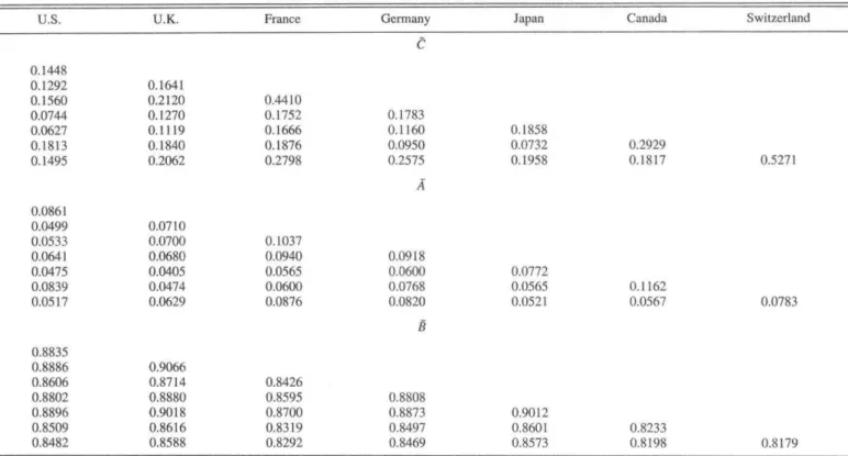
TABLE 2.—PARAMETER ESTIMATES OF THE FLEXM MODEL
U.S. U.K. France Germany Japan Canada Swilzerland
0.1448 0.1292 0.1560 0.0744 0.0627 0.1813 0.1495
0,0861 0.0499 0.0533 0.0641 0,0475 0.0839 0.0517
0,8835 0.8886 0.8606 0.8802 0,8896 0.8509 0.8482
0,1641 0.2120 0.1270 0.1119 0.1840 0.2062
0.07 to 0.0700 0.0680 0.0405 0.0474 0.0629
0.9066 0,8714 0.8880 0,9018 0.8616 0.8588
0,4410 0.1752 0.1666 0.1876 0.2798
0.1037 0.0940 0.0565 0.0600 0.0876
0,8426 0.8595 0.8700 0.8319 0.8292
0.1783 0.1160 0.0950 0.2575
A
0.0918 0.0600 0.0768 0.0820 a a
0,8808 0.8873 0,8497 0,8469
0.1858 0,0732 0,1958
0,0772 0.0565 0,0521
0.9012 0.8601 0.8573
0.2929 0.1817
0.1162 0.0567
0,8233 0,8198
0.5271
0.0783
0.8179
This table presents the estiinaied paramciers ol the flexible multivariate (Re!£M)GARCH(l,l) model ba.'ied on Ihe entire sample. The model is developed and described in section U. As ihe matrices are sytnmetric. only (he lower triangular parU are displaytd to enhance readability.
Rolling Window: The ever popular rolling-window es-timator simply estimates the covariance matrix at time t, conditional on the information available at time t — 1, as the sample covariance matrix of the observations x,-^, . . . , x,-i, where k is some predetermined integer. A common choice for weekly data \sk — 104, which corresponds to a 2-year window. In the remainder of the paper, this model will be called Window.
Exponential Smoothing: The exponential smoothing es-timator is given by
H, ~ \x,_|X,V| -f
where X is a small, positive constant. Note that this pre-scription requires some suitable starting values. A common approach is to use the rolling-window estimator at time k + 1 f o r ^ , , . . . , H , + i.
The exponential smoothing estimator corresponds to a muitivadate integrated GARCH(1,1) model with a unique autoregressive coefficient (1 ~ \ ) and a unique moving-average coefficient (X) for all variances and covariances. This specification is the basis of many risk measurement systems currently in use and, for example, is advocated by RiskMetrics. A commonly used value for X is 0.06. In the remainder of the paper, this model will be called RiskM.
C. Estimation of the Models
When estimating the three muitivadate GARCH(1,1) models from the entire set of 1,356 weekly data, the
esti-mation of the FlexM model took less than three minutes, using a proprietary optimization routine in Matlab. In con-trast, the estimation of both the CCC and the BEKK model took over one hour, using off-the-shelf optimization routines available in Matlab. Tables 2-5 present the estimates of the parameters of the various models. Table 3 displays bootstrap standard errors for the FlexM model.
However, we do not use these estimated models in our comparisons, as this strategy would focus on the in-sample performance of the various estimators. In-sample compari-sons are not ideal for our purposes, for at least two reacompari-sons. First, they are too optimistic, because the entire sample is used in the fitting process before the fitted models are then applied in hindsight. Second, they tend to favor models with more degrees of freedom, so FlexM might have an unfair advantage.
We will therefore use out-of-sample comparisons in what follows. In general, the forecasts for time t are made using information available up to time t - I only. The parameter estimates of the multivariate GARCH(1,1) models are up-dated every four weeks to reduce the computational burden for BHKK and CCC. All forecasts start at time t = 601.
D. Forecast Criteria
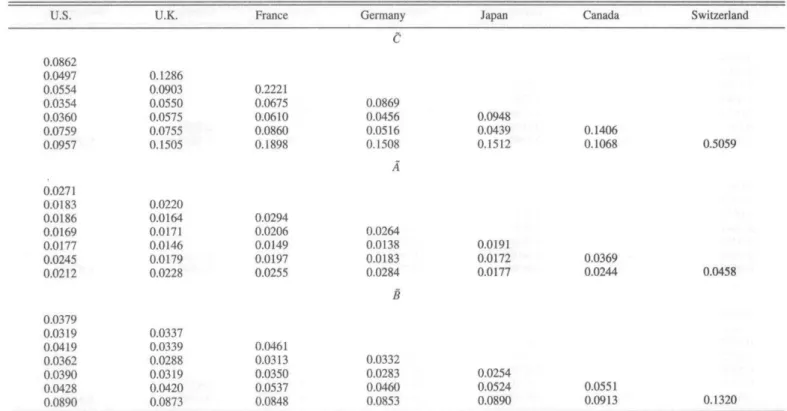
TABLE 3,—STANDARD ERRORS OF THE FLEXM MODEL
U,S. U.K. France Germany Japan Canada Switzerland
0.0862 0.0497 0.0554 0.0354 0.0360 0.0759 0.0957
0.0271 0.0183 0.0186 0,0169 0.0! 77 0.0245 0.0212
0,0379 0.0319 0.0419 0.0362 0.0390 0.0428 0.0890
0.1286 0.0903 0.0550 0.0575 0.0755 0.1505
0.0220 0.0164 0.0171 0.0146 0.0179 0.0228
0.0337 0.0339 0.0288 0.0319 0.0420 0.0873
0,2221 0.0675 0,0610 0,0860 0.1898
0,0294 0,0206 0,0149 0,0197 0.0255
0.0461 0.0313 0.0350 0.0537 0.0848
0.0869 0.0456 0.0516 0.1508
A
0.0264 0.0138 0.0183 0.0284
B
0,0332 0.0283 0.0460 0,0853
0.0948 0.0439 0.1512
0,019] 0,0172 0,0177
0.0254 0.0524 0.0890
0,1406 0.1068
0,0369 0,0244
0.0551 0.0913
0.5059
0.0458
0,1320
lliis lable pre.'^nt'; bootstrap siandatd errors corresponding lo (he parameter esiimaies of lable 2. The standard errors were computed as outlined in algorithm I, using K = 100. As the matrices are symmetric, only the lower manguiar parts are di.splayed to enhance readability.
cumulative cross-products of intraday return residuals over the forecast horizon; for example, see Andersen, Bollerslev, and Lange (1999) (henceforth ABL) or Andersen, Boller-slev, Diebold, and Labys (2001). Unfortunately, we only have daily return data available, but the same methodology can be applied to them; this results in a less precise but still useful proxy. We consider forecast horizons of 1, 2, and 4 weeks. Note that there are standard formulas to compute the 2-week and 4-week forecasts for multivariate GARCH models, given the 1-week forecast and the estimated model
at time / - 1; for example, see ABL. To compute the 2-week and 4-week forecasts for RiskM and Window, we simply multiply the 1-week forecasts by the forecast hori-zon. Denote by (i,^k the estimated conditional covariance matrix, based on the information available at time t — 1, for the (t-week forecast horizon; in this notation ^,,i corre-sponds to fi,, the 1-week forecast. Also, let X,.fc be the cumulative cross-products of daily return residuals during that period. The typical elements of these two matrices are denoted by ^y.i,^ and <Jij,t,ky respectively. As do ABL, we
TABLE 4.—PARAMETER ESTIMATES OF THE CCC MODEL
U.S. U.K. France Germany Japan Canada Switzerland
0,1850 0.0733 0.3495
Cii
0,1514 0.2356 0.2992 0.5743
0.0700 0.0520 0.0731 0.0446 0.0727 0.0898 0.0467
0.8872
J.OOOO 0,4392 0.3572 0.3302 0.2469 0,6753 0,3655
0,9379
1.0000 0.4888 • '
0,4623
0.3369 . • 0.4352 0.4852
0.8819
- 1.0000 • 0.5643 0,3373 0,3459 0,5299
0.9278
Correlation Matrix
l.OCXX) 0.3688 0.3267 0,7009
0.S977
l.OOOO 0.2244 0.3891
, U.844i
1.0000
0.3450 l.OOOO
TABLE 5.—PARAMETER ESTTMATES OF THE B E K K MODEL
U.S. U.K. France Germany Japan Canada Switzerland
G
0.3034 0.1004 0.1508 0.1291 0.0842 0.2408 0.2039
0.1446
0.9786
0.1662 0.2863 0.2558 0.1154 0.0831 0.3923
0.1283
0.9885
0.2634 0.0215 0.0374 -0.0329 -0.0519
0.214t
0.9657
0.2696 0.0561 -0.0270 0.0905
Diag (E)
0.2050
Diag (F)
0.9655
0.3300 -0.0060 0.0557
0.1709
0.9769
0.2485 -0.0620
0.1567
0.9729
0.2302
0.1872
0.9557
This table presents the eslimaled parameleis of the diagonal BBKK GARCH(l.i) mode! based on the enlire sample. The model is de.scribed in ihe second part of section IIIB. Nole thai G is a lower triangular matris, .so ihe elenienis not displayed are equal to zero.
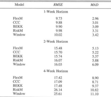
consider the following two criteria to judge the quality of (two criteria and three horizons). FlexM is best four times the volatility forecasts: (for both criteria at the 1-week and 2-week horizons), and CCC is best two times (for both criteria at the 4-week
RMSE, - 77^ ,, , . horizon). RiskM and Window are always worse than the
multivariate GARCH models.
(15)
and MAD^ are multivariate versions of the root-mean-square error and mean absolute deviation, respec-tively. Criteria based on absolute deviations are sometimes preferred (as, for example, in ABL), because they are more robust and less affected by a few large outliers.
Table 6 reports estimates of the two criteria at the differ-ent forecast horizons. There are six comparisons altogether
TABLE 6.—FORECAST CRITERIA FOR COVARIANCE MATRICES
Model
FlexM
CCC BEKK RiskM Window
FlexM
CCC BEKK Ri.skM Window
FlexM CCC BEKK RiskM Window
RMSE
1-Week Horizon
9.73 9.88 9.90 9.98 10.02
2-Week Horizon
15.48 15.70 15.74 16.07 16.03
4-Week Horizon
17.42 17.09 17.48 26.14 25.61
MAD
2.96 3.01 3.09 3.31 3.42
5.13 5.22 5.37 5.88 6.09
8.90 8.71 9.37 10.82 11.10
E. Standardized Residuals
Consider the standardized residuals e, = HJ^'^Xt, where
H, is the true conditional covariance matrix at time t.
Obviously, the e, have constant conditional covariance ma-trix equal to the identity, and the cross-products e,e,' are uncorrelated over time. It is therefore natural to test for any left-over autocorrelation in the cross-products e,ej, where €, = fi'^^'^x, and H, is the estimated conditional covariance matrix at time t.
A standard test for serial correlation in a univariate time series {y,} is the Ljung-Box test. The test statistic is
m.
/=!
This table compares ihe forecasted conditional covariance matrices with the realized integrated volatility covariance matrices computed from daily data that serve as a proxy for Ihe true bul unobservabie cotidiiional covariance matrices. The criteria RMSE and MAD are defined in equations (I4M15). All forecasts are out of sample. Forecasts start at week / = 601,
where p(/) is the sample autocorrelation of order /, and k is an integer which is small compared to the sample size T.
The commonly used asymptotic null distribution is xl^ the c/i(-squared distribution with k degrees of freedom.
There are, however, two problems with applying this test for our purposes. A general problem is that the asymptotic null distribution is only correct under the additional assump-tion of i.i.d. data. If the series {y,} is uncorrelated but dependent, the x* approximation can be arbitrarily mislead-ing (Romano and Thombs, 1996). Another problem is that the test is designed for univariate series and not series of
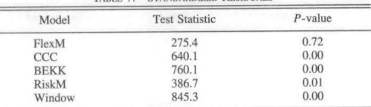
TABLE 7.^STANDARDIZED RESIDUALS
Model
FlexM CCC BEKK RiskM Window
Test Statistic
275.4 640.1 760.1 386.7 845.3
P-value
0.72 0.00
0.00 0.01
0.00
« table presents lest results for left-over autocorrelatLon in the titled standard [zed residuals. The test statistic is the combined Ljung-Box statistic defined in equation (16) using the lirst * = 12 sample autocorrelations. The /"-value for the nnll hypothesis of no autocorrelation is obtained hy applying the suhsan^jling method with block size h ~ 100, as detailed in the discussion following equation (16). All fitted standardized residuals are out of sample and are computed starting at week i = 601.
The combined test statistic we suggest is
(16)
where LBij{k) is the univariate Ljung-Box test statistic computed from the series {e;,,ey,,}. To assess the evidence against the null hypothesis, we compute the P-value based on the subsampling method. To this end, let EB^omb,,,b(^) be the combined test statistic based on the stretch of data
[i, , it+h-\}^ foTt= 1 T - b + 1. Here, the block size b is an integer smaller than T. The subsampling P-value is then given as
By arguments analogous to the ones of Romano and Thombs (1996), it can easily be shown that this test is consistent if the cross-products are uncorrelated but depen-dent. For more details about the general use of subsampling tests with dependent data, the reader is referred to Politis, Romano, and Wolf (1999, chapter 3). The block size b needs to satisfy the asymptotic conditions b -^ ^ and b/T -^ 0; some methods for choosing b in practice are given in Politis, Romano, and Wolf (1999, chapter 9).
Table 7 presents the test statistic and corresponding /'-value for the five models, using/: = 12andfo= 100; the results are similar for other values of k and b. FlexM has the smallest test statistic and is the only model that is not rejected at any conventional level; its P-value is 0.72, the one for RiskM is 0.01, and all the others are 0.
F Value at Risk
An important use of the conditional covariance matrix is in calculations of the value at risk (VaR) of a portfolio of assets. A large number of methods to compute the VaR have been suggested and are currently employed, such as histor-ical simulation, RiskMetrics, Monte Carlo, GARCH, non-parametric quantile regressions, and methods based on extreme-value theory. We certainly do not aim to settle the dispute as to which method is best, and it stands to reason that a uniformly best method does not exist. However, GARCH methods are very popular among practitioners and tend to perform well. (In particular, recent claims that they
are dominated by methods based on extreme-value theory do not seem to be substantiated; for example, see Lee and Saltoglu, 2001.)
If a single portfolio is considered, it makes more sense to fit a univariate GARCH(1,1) model to the corresponding return series and base any VaR calculations on this model. On the other hand, if a number of different portfolios based on the same universe of A^ assets are considered (as is the case with different traders of an investment bank, say), it is common practice to base the individual VaR calculations on a single estimate of the conditional covariance matrix of all
N assets. This also allows computing the marginal contri-butions to risk of each position and evaluating the effect of hedges. Hence, multivariate GARCH is certainly relevant to risk management applications.
In our tests, we consider the following four portfolios based on the seven market indices that make up our data:
• U.S. portfolio: United States only.
• North American portfolio: United States and Canada equally weighted.
• European portfolio: United Kingdom, France, Ger-many, and Switzerland equally weighted.
• Worid portfolio: all seven countries equally weighted.
We use the estimated conditional covariance matrix to compute the one-week-ahead VaR at levels 1% and 5%. In order to try to fit the tails of the return distributions and to match the theoretical VaR levels, we assume a conditional r-distribution. To be more specific, let the portfolio be represented by the vector of weights, w. The estimated conditional variance of the portfolio at time t is then given by
At time t - 1, we condition on the past portfolio returns and their corresponding estimated conditional variances to choose the number of degrees of freedom, v*, that maximizes the likelihood ..
-r - l
n
r(v/2)
(w'x,]over V, where r(-) denotes the gamma function. Note that the standard formula for the r-distribution has been modi-fied by the scale factor ^^,,(v - 2)/v, where the degree-of-freedom adjustment is designed so that /j^.., is exactly equal to the conditional variance of w'xj. Having thus found V*, the 1% VaR at time / is finally computed as
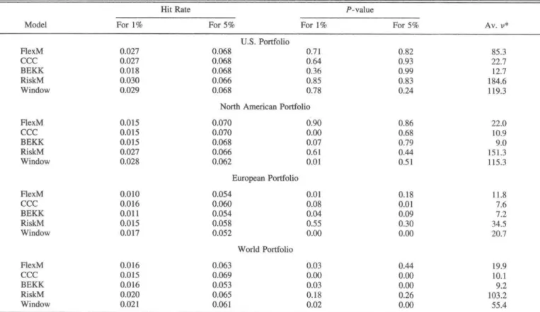
TABLE 8.—VALUE AT RISK
Hit Rate P-value
Model For 1% For 5% For 1% For 5% Av. V*
FlexM CCC BFKK RiskM Window FlexM CCC BEKK RiskM Window FlexM CCC BEKK RiskM Window FlexM CCC BEKK RiskM Window 0.027 0.027 0.018 0.030 0.029 0.015 0.015 0.015 0.027 0.028 0.010 0.016 0.011 0.015 0.017 0.016 0.015 0.016 0.020 0.021 U.S. Portfolio 0.068 0.068 0.068 0.066 0.068 0.71 0.64 0.36 0.85 0.78
North American Portfolio
0.070 0.070 0.068 0.066 0.062 European Portfolio 0.054 0.060 0.054 0.058 0.052 World Portfolio 0.063 0.069 0.053 0.065 0.061
0 . ^ 000 0.07 0.61 0.01 0.01 0.0g 6.04 0.55 0.00 0.03 0.00 0.03 0.18 0.02 0.82 0.93 0.99 0.83 0.24 0.86 0.68 0.79 0.44 0.51 0.18 0.01 0.09 0.30 0.00 0.44 0.00 0.00 0.26 0.00 85.3 22.7 12.7 184.6 119.3 22.0 10.9 9.0 151.3 115.3 11.8 7.6 7.2 34.S 20.7 19.9 10.1 9.2 103.2 55.4
This table compares VaR calculations al ieveU 1% and 5%. assuming a condilional r-distfibulion (suilably normaJized}. TTie hit rate is the sample mean of the hit series defined in equation (17) and should be close lo the nominal level. The P-value corresponds to ihe null hypothesis of no autocorrelation in the hii series and is obtained from the usual r/i/-squared approximation of the univaiiate Ljuug-Bos lest statislic tising the first * = 12 sample autocorrelations. The last column shows the average optima! number of degrees of freedom, v", for the conditional /-distribution. Ail VaR calculations are out of sample and star! al week ( = 601.
For a certain portfolio and for a given level, define the hit variable
hit, = I{w'x, < VaR,}, (17)
where /{•) is the indicator function and VaR, is the esti-mated VaR at time t. If the model to calculate the VaR is correctly specified, the series [hit,] should be uncorrelated over time and have expected value equal to the desired nominal level.
Table 8 presents the sample means (or hit rates) and the Ljung-Box P-values for autocorrelation of the hit series for the various methods, portfolios, and VaR levels. The P-values are based on the first k = \2 sample autocorrela-tions. Because the hit series are univariate and because a (stationary) {0, 1} series is uncorrelated if and only if it is independent, it is safe to use the asymptotic cAi-squared approximation to compute the P-values here. (The table also presents the average optimal number of degrees of freedom, v*, of the conditional /-distribution.)
The hit rates are all reasonably close to the target levels, although they tend to be a bit larger on average. There is no clear winner or loser in terms of the hit rates. Judging the serial correlation of the hit series [hit,], it is seen that RiskM performs best: all its P-values are above 0.1. FlexM is somewhat better than the other GARCH models.
G. Portfolio Selection
Another important application of the conditional covari-ance matrix is as an input to the Markowitz (1952) portfolio selection method. Hence, we examine the gains from inter-national diversification obtained by taking into account the time-changing nature of the covariance matrix. In order to avoid having to specify the vector of conditional expected returns, which is more a task for the portfoHo manager than a statistical problem, we focus on constructing the (global) minimum-variance portfolio, allowing for short sales.
Table 9 shows the realized (annualized) standard devia-tion of the returns of the condidevia-tional-minimum-variance
TABLE 9.—STANDARD DEVIATION OF PoRTFOLio RETURNS
Portfolio
U.S.
Equal-weighted world
Unconditional minimum-variance FlexM minimum-v^ance CCC minimum-variance BEKK mini mum-variance RiskM minimum-variance Window minimum-variance Standard Deviation 15.87 13.33 12.91 12.32 12.53 12.54 13.37 12.89
portfolio over the entire sample period, obtained from the three GARCH models, the RiskMetrics method, and the rolling-window method. It compares them with the standard deviation of the U.S. stock market, of the equal-weighted portfolio of the seven stock markets, and of the uncondi-tional minimum-variance portfolio obtained from the sam-ple covariance matrix at t = 1,356. (The last portfolio would be infeasible, but we include it nevertheless.) Not surprisingly, fully investing in the U.S. stock market yields the highest standard deviation, followed by the equal-weighted world portfolio and the unconditional minimum-variance portfolio. All three GARCH models provide a significant improvement, with RexM being the best. Win-dow is comparable to the unconditional minimum-variance portfolio, and RiskM is worse than even the equal-weighted portfolio.
IV. Conclusion
In this paper, we have developed an estimation procedure for the general diagonal-vech formulation of the multivari-ate GARCH(1,1) model. Our procedure is the first to be computationally feasible for dimensions N > 5, without constraining the coefficient matrices. Our method proceeds in two steps: first, we decentralize the problem by estimat-ing separately N univariate and A'^(A'^ — l)/2 bivariate GARCH models, all of which are computationally feasible problems; second, we bring together these results to form iV-dimensional matrices of parameter estimates, which we transform in order to ensure the positive semidefiniteness of the conditional covariance matrices. In doing so, we avoid having to impose additional restrictions, which has been the common approach so far in the multivariate GARCH liter-ature. In addition, our method is computationally far less demanding than traditional multivariate models, which is an important advantage if the sample size is large, as would be the case with high-frequency data.
We apply our procedure to 25 years of weekly data on seven major national stock markets and compare it with two popular traditional multivariate GARCH( 1,1) models, namely the constant-conditional-coirelation mode! and the diagonal BEKK model, and with two widely-used, albeit less sophisticated, estimators, namely the rolling-window estimator and the exponential smoothing estimator. Using a number of criteria, such as forecast accuracy, persistence of standardized residuals, precision of value-at-risk estimates, and optimal portfolio selection, we find that the flexible multivariate GARCH method does indeed offer improved performance. The use of high-frequency data, which un-doubtedly will increase in the future, should make our procedure even more attractive.
Direct applications of this method involve portfolio se-lection and tests of asset pricing models such as the inter-national CAPM, and risk measurement uses such as the value at risk. An interesting topic left for future research is an extension to asymmetric multivariate GARCH{1,1).
REFERENCES
Andersen, Torben G., Tim BoHersIev, Frank X. Dieboid, and Paul Labys, "The Distribution of Realized Exchange Rate Volatility," Journal of the American Statistical Association 96 (2001), 42-55. Andersen, Torben G., Tim Bollerslev, and Steve Lange, "Forecasting
Financial Market Volatility: Sample Frequency vis-^-vis Forecast Horizon," Journal of Empirical Finance 6 (1999), 457-177. Bolierslev, Tim. "Modelling the Coherence in Short-Run Nominal
Ex-change Rates: A Multivariate Generalized ARCH Model," this REVIEW 72 (1990), 498-505.
Bollerslev, Tim, Robert F. Engle, and Jeffrey M. Wooldridge, "Capital Asset Pricing Model with Time-Varying Covariances," Journal of Political Economy 96 (1988), 116-131.
Campbell, John Y., Andrew W. Lo, and A. Craig MacKinlay, The Econo-metrics of Financial Markets (Princeton: Princeton University Press. 1997).
Ding, Zhuanxin, and Robert F. Engle. "Large Scale Conditional Covari-ance Matrix Modeling, Estimation and Testing," University of California mimeograph, San Diego (1994).
Efron, Bradley, and Robert J. Tibshirani. An Introduction to the Bootstrap
(New York: Chapman & Hall, 1993).
Engle, Robert, "Dynamic Conditional Correlation: A Simple Class of Multivariate Generalized Autoregressive Conditional Heteroske-dasticity Models." Joumal of Business and Economic Statistics
20:3 (2002). 339-350.
Engle, Robert F., and Kenneth Kroner, "Multivariate Simultaneous GARCH," Econometric Theory II (1995), 122-150.
Engle, Robert F., and Joseph Mezrich, "GARCH for Groups," Risk 9
(1996). 36-40.
Lee, Tae-Hwy, and Burak Salloglu, "Evaluating the Predictive Perfor-mance of Value-at-Risk Models in Emerging Markets: A Reality Check." University of California mimeograph. Riverside (2001). Markowitz, Harry, "Portfolio Selection," Joumal of Finance 7 (1952),
77-91.
Politis. Dimitris N., Joseph P. Romano, and Michael Wolf, Subsampling
(New York: Springer, 1999).
Romano, Joseph P.. and Lori A. Thombs, "Inference for Autocorrelations under Weak Assumptions," Joumal of the American Statistical Association 91 (1996), 590-600.
Sharapov, llya, "Advances in Multigrid Optimization Methods with Ap-plications," University of California, PhD dissertation, Los Ange-les (1997).
Styan, George P. H., "Hadamard Products and Multivariate Statistical Analysis." Linear Algebra and Its Applications 6 (1973), 217-240.
A APPENDIX
-'-,.:',. , Minimization of the Frobenius Norm . -1. Problem Formulation
Given a symmetric matrix A with the property diag (A) > 0. find a symmetric, positive semidefinite matrix M with diag (M) = diag (A) that minimizes [[A — M\\F, where || - ||/.- is the Frobenius norm.
"• -"- ' 2. Numerical Solution • ' - '
Write the matrix A and the current approximation A/ to the solution of the above problem as
a,, a' a A J
an m'
m M
and let the conditions of the problem be satisfied [that is, diag (A/) = diag (A) and A/ = A/^ > 0]. For a matrix of the form
P ^'
M =
If we enforce the condition
- 2p.j:'^»i + x^Hdx pm^ + x'^i
pm + Mx M (A-l)
(A-2)
then the new approximation fvf satisfies the conditions of the problem: A? = M^ a 0 and diag (Kl) = diag {A).
If equation (A-2) is satisfied, we have
\\A - fk\\r - \\A - M\\, = 2\\a - (pm - 2\\a
-therefore, choosing x and p that minimize \\a - (pm + MJ:)||2, from equation (A-2) we get A? that minimizes ||i4 — A^Wf, satisfies the conditions of the problem, and is obtained from the previous approxima-tion M by changing its first row and column. The extension to the /* column and row is obvious.
Remark 1. The convexity of the problem implies that the solution matrix M is singular, that is, lies on the boundary of the feasible region. Since det (Af) = p^ det (M), we can make the iterates stay within the interior of the feasible region by initializing the process with a nonsingular matrix and choosing p to be bounded away from 0. Later on we treat p as a chosen constant between 0 and I, so the iterates become singular no faster then expionentialty. In numerical examples, p is chosen to be 0.5.
One step of the iterative procedure becomes
min ||a ~ (pm + Jtf.)c)|}2
subject to equation (A-2); introducing
b = a — pm,
it becomes
still subject to equation (A-2).
The Lagrangian of this subproblem is
L{x, \) - \\Mx - bf^ + Up^a^i + 2p^^m and the optimality conditions are
F{x) = p^o,| + Ipx^m +x^Mx- a,, = 0 and
, \) = 6,
- a,,).
(A-3)
which can be written as
Mh - Mb + \pm + \Mx = 0.
For any \ , equation (A-4) can be solved for x: x(\) = (M- + kM)-'{Mb - Xpm); and
n\) = F{x{\)) = Q
can be solved by the Newton's method:
(A-4)
(A-5)
The analytic expression for f ^(X) can be obtained from
F,(k) = V,F(x) • ;c, = 2(pm + Mx)^
By differentiating equation (A-4) with respect to \ we get
Mh^ + pm + Mx + xMxi, = 0; therefore
(A-7)
Inserting this in equation (A-7), we get
F,(X) = ~2(pm + Mx)^(M^ + XM)-'(pm + Mx). (A-8)
We can summarize the solution of the subproblem as:
1. Initialize X (say X = 0). 2. Compute x by equation (A-5).
3. Compute F(\) and F,^(X) using equations (A-3) and (A-8). 4. Update \ using Newton's step (A-6).
5. Recur Newton's procedure.
Remark 2. The steps (A-3) and (A-8) involve the inverse of M^ + KM,
which is singular if M is. Restricting p to be a nonzero constant results in nonsingular M unless it is a solution; see remark I.
A Matiab routine implementing this procedure has been written by Ilya Sharapov and is available from the authors upon request.
3. Numerical Tests