exchange rate and inflation volatilities
∗
Christiane R. Albuquerque
†
, Marcelo S. Portugal
‡
Contents: 1. Introduction; 2. The theoretical model; 3. Data; 4. Tests with unconditional volatility; 5. Tests with conditional variance – Bivariate GARCH; 6. Conclusions; A. Tables & Graphs; B. Diagnostic Tests for the Bi-Garch Model.
Keywords:Exchange rate, inflation, volatility, Garch models
JEL Code:E31, F41.
There are few studies, directly addressing exchange rate and inflation volatilities, and lack of consensus among them. However, this kind of study is necessary, especially under an inflation-targeting system where the monetary authority must know well price behavior. This article analy-ses the relation between exchange rate and inflation volatilities using a bi-variate GARCH model, and therefore modeling conditional volatilities, fact largely unexplored by the literature. We find a semi-concave relation be-tween those series, and this nonlinearity may explain their apparently dis-connection under a floating exchange rate system. The article also shows that traditional tests, with non-conditional volatilities, are not robust.
Existem poucos estudos, e pouco consenso, sobre a relação entre as volatil-idades cambial e da inflação. Todavia, tais estudos são necessários, especial-mente em um regime de metas de inflação onde a autoridade monetária deve conhecer detalhadamente o comportamento dos preços. Existem poucos estu-dos, e pouco consenso, sobre a relação entre as volatilidades cambial e da in-flação. Todavia, tais estudos são necessários, especialmente em um regime de metas de inflação onde a autoridade monetária deve conhecer detalhadamente
∗The authors would like to thank Carlos H. V. Araújo (Banco Central do Brasil – BCB), Joaquim de Andrade (UNB), Maria da Glória Araújo (BCB), Roberto Camps de Moraes (UFRGS), Sergio Alves (BCB) and an anonymous referee for their comments on a previous version. The authors also would like to thank Angelo Fasolo and Eui Jung (both from BCB) for their valuable contributions to this paper. The remaining errors are the authors’ responsibility. The views expressed in this work are those of the authors and do not necessarily reflect those of the Central Bank of placecountry-regionBrazil or its members.
†Economist, Research Department of the Central Bank of placecountry-regionBrazil. E-mail:❝❤r✐st✐❛♥❡✳❛❧❜✉q✉❡rq✉❡❅❜❝❜✳
❣♦✈✳❜r
‡Professor of Economics, Universidade Federal do Rio Grande do Sul (UFRGS), and associate researcher of CNPq. Email:♠s♣❅
o comportamento dos preços. Este artigo analisa a relação entre aquelas idades usando um modelo Garch bivariado, modelando, portanto, as volatil-idades condicionais, enfoque pouco explorado pela literatura. Encontramos uma relação semi-côncava entre as séries, e esta não-linearidade pode explicar o aparente descolamento das mesmas em períodos de regime cambial flutu-ante. O artigo também mostra que os testes tradicionais, com volatilidades não-condicionais, não são robustos.
1. INTRODUCTION
The study of exchange rate volatility’s effects should be important for monetary policy decisions, since higher volatility means higher uncertainty, which may affect inflation expectations, a crucial vari-able in monetary policy decisions. Although the literature about the impact of exchange rate volatility on inflation is not as extensive as the one available for its pass-through to prices, some authors high-light such relation. Whether the impacts are significant or not remains controversial: some authors de-fend the absence of connection between exchange rate and macroeconomic variables volatilities while others state the opposite.1 According to the first group, exchange rate volatility is not important to
macroeconomic variables, since empirical evidence shows a substantial increase in the former during floating exchange rate regimes, while the latter did not present a similar rise in their volatilities.2The
second group finds evidence of such relation, being either positive or negative, in studies conducted under different aims and approaches.
This paper seeks to check for the existence of a relation between exchange rate and inflation volatil-ities for the Brazilian case, and our conclusions in this paper could be classified in the second group, related especially with the findings of Dixit (1989) and Seabra (1996). By developing an optimization model for the firm, the first author shows that trade flows and prices would depend on investment made on a future basis and, consequently, on both expectations and higher moments of the distribu-tions involved. In consequence, the macroeconomic environment affects the pattern of price changes. Hence, not only the level of the devaluation but also the volatility of the exchange rate would affect its pass-through to prices. Seabra (1996), on its turn, uses a model of intertemporal optimization with asymmetric adjustment costs and shows that the critical value that leads a firm to invest is a function of uncertainty. If uncertainty is high, the optimal decision will be to wait before making a movement (wait-and-seestrategy), even with the exchange rate at a level that makes investment profitable. This attitude impacts on aggregate supply and, therefore, on inflation.
Other interesting works are those of Hausmann et al. (2001), who find a negative and significant correlation in their tests between pass-through and measures of volatility, and Smith (1999), where a reduction in inflation volatility as a result of an increase in exchange rate volatility was found in approximately 31% of the cases. The welfare approach recalled by Ghosh et al. (1997) and by Sutherland (2005) are also worth mentioning. The former show that inflation volatility is lower under floating and intermediate exchange rate regimes for countries with low inflation, while the latter show that the sign of relation between exchange rate and inflation volatilities will depend on the model’s parameters.
In this paper, we adopt a more sophisticated econometric methodology than those applied so far in literature: instead of constructing exogenous volatility series (by computing the volatility of subsamples
1For the first group, see, for instance, Krugman (1988), Obstfeld and Rogoff (2000), Baxter and Stockman (1988), Flood and
Rose (1995), Rogoff (2001) and Duarte and Stockman (2002). For the second, Calvo and Reinhart (2000a,b), Barkoulas et al. (2002), Wei and Parsley (1995), Andersen (1997), Smith (1999), Engel and Rogers (2001), Devereux and Engel (2003), Chen (2004), Barone-Adesi and Yeung (1990), Bleaney (1996), and Bleaney and Fielding (2002).
2Obstfeld and Rogoff (2000) call the apparently disconnection between the exchange rate volatility and macroeconomic
or rolling windows) we apply a bivariate GARCH model, working with conditional volatility series. The purpose of this procedure is to adopt a measure not sensitive to individual selection criteria. Apart from that, by modeling the conditional heteroskedasticity of exchange rates, it is also a more suitable econometric technique. One of the contributions proposed by this paper is to verify whether exchange rate volatility has impacts strong enough on inflation so that the monetary authority should monitor it, an approach still scarce, especially in placecountry-regionBrazil. The other one is to show that traditional tests are not robust for this type of study and that Garch-type models are more suitable for such analysis.
The paper is divided into six sections, including this introduction. Section 2 introduces the theoret-ical model that led to the econometric tests, while data is presented in section 3. The results obtained by the use of traditional methods (i.e.: unconditional variance series) are presented in section 4. Section 5 shows the results of the bivariate GARCH model, and section 6 concludes.
2. THE THEORETICAL MODEL
We derive an equation relating inflation and exchange rate volatilities to test for the existence of a significant relation between them. The approach to achieve such equation is based on Bleaney and Fielding (2002), with slight modifications. The government has a utility function Z, of the Barro and Gordon (1983) type, to be maximized. Z is given by equation 1, which represents the case where the government of a country faces a trade-off between price stabilization and output growth above its equilibrium level.
Z =−0.5π2−0.5b(y−y∗−k)2 (1)
Whereπis inflation,yis the output level andy∗is potential output. The termb >0is incorporated
by the authors, meaning the relative weight given to output, andk > 0 represents the inflationary bias of the government. The presence ofbandkcomes from the assumption that a government could eventually attribute a higher weight to output growth to the detriment of price stability.
The restriction imposed by the authors upon functionZ consists of an expectations-augmented Phillips Curve, including the exchange rate. Here, we have the first difference to the model of Bleaney and Fielding (2002) since we will focus not on the real but on the nominal exchange rate. Our restriction will be a Phillips Curve for an open economy, including both the forward-looking and the backward-looking term, as described in equation 2 below.
πt=a0πet+a1πt−1+a2(y−y∗) +a3∆(ptext) +a4st+ǫt (2)
wherepext
t is the foreign price level,st, the nominal exchange rate andπet the inflation expectation
between periodtand periodt+ 1.
We also assume the exchange rate following a random walk, as in many partial equilibrium studies. Thus, we have
st=st−1+ηt ηt∼N(0, σ2η) (3)
applying (2) and (3) to (1), and obtaining the first-order condition for the maximization ofZwith respect toπ, we have
π=βa0πet+βa1πt−1+βa3∆ptext+βa4st−1+βa4ηt+βǫt+K′ (4)
whereβ= b a2
2+b
andK′=−βa2k.
Some assumption also must be made concerning the behavior ofπe
t. We, then, consider that
infla-tion expectainfla-tions are of the form:
Thus, substituting (5) in (4) we get that
E[π] = (βa0+βa1)πt−1+βa3∆pextt +K′ (6)
The termsǫt,ηtandνtare independents, therefore, inflation variance given by
var(π) =β2a20E(υt)2+β2a24E(ηt)2+β2E(ǫt)2 (7)
But, from (2), we have thatE(ǫt)2is the inflation variance. Hence,
var(π) =µ0E(υt)2+µ1E(ηt)2 (8)
whereµ0= β
2
a2 0
(1−β2)andµ1=µ0∗
a2 4
a2 0
Inflation variance is, therefore, a function ofνt(the variance of the shock expected intin relation
tot−1inflation) and ofηt(variance of the exchange rate process).
With (8), we may test for a relation between volatilities and we aim to do that by using a multi-variate GARCH model. However, due to the small sample available – from the beginning of the floating exchange rate system in placecountry-regionBrazil, i.e., January, 1999 to September, 2004 – the large number of terms to be estimated does not allow us to estimate a multivariate GARCH model with three variables. Aside from that, the inflation expectations research published by the Central Bank of placecountry-regionBrazil started only on April, 2000, reducing our sample even further. Therefore, we will assume that the variance measured byνtis constant and, hence, equation 8 becomes:
V ar(π) =µ′
0+µ1var(ηt),
whereµ′
0=µ0+var(νt)is the new constant.
Although the assumption that νt is constant is strong, we may consider it. Table 1 shows the
result of a regression ofπe
t againstπt−1and a constant. If our hypothesis that the shock expected to
t+ 1in comparison witht−1is, on average, constant, then the residuals of this equation should be homoskedastic. As we may see, we accept the null hypothesis of homoskedasticity, which supports our assumption thatνtis constant.3 Besides, if we computevt=πet−πt−1one can notice that almost the
entire series is within the interval of one standard deviation from the mean, as shown in Graph 1, with the longest period in which it was outside that band being from December 2002 to April 2003.
The data forπe
t refer to the average market expectations for IPCA4inflation in montht+ 1as in the
last business day of montht−1, and they are published by the Investor Relations Group (Gerin) from the Central Bank of Brazil.5
Table 1 –Estimation of Equationπet =c+πt−1
method: OLS; sample: 2000:03 to 2004:10
Variable Coefficient Standard deviation t−statistics p−value
πt−1 0.1593 0.0542 29.385 0.0049
C 0.4463 0.0555 80.351 0.0000
MA(1) 0.6576 0.1145 57.452 0.0000
R2 0.4584 Durbin-Watson 18.755
adjustedR2 .4376 White Test for homoskedasticity: (p-value) 0.4354
3Equivalent tests toπ
tandstfrom equations 2 and 3 accepted the alternative hypothesis of heteroskedasticity.
4Index of consumer prices considered by the Central Bank in the inflation targeting.
Figure 1 –Evolution ofνt=πe−πt−1
3. DATA
Our sample was computed on a monthly basis, from 1999:01 to 2004:09, and data used in our estimations were the following:
(a) Price Index: Extended Consumer Price Index (IPCA), consumer price index published by the Brazilian Institute of Geography and Statistics (IBGE),6December/1993=100 and considered by the Central
Bank of Brazil as the reference index in the inflation targeting regime;
(b) Exchange Rate: Exchange rate R$/US$, selling prices, monthly average;
(c) External Prices:Producer price index(PPI), published by theBureau of Labour Statistics7(commodities,
final goods).
(d) GAP: output gap. It was computed by subtracting the industrial production series published by IBGE (used as aproxyfor monthly GDP) from the trend obtained by the Hodrick-Prescott filter.
All series were seasonally adjusted by the X-12 method and, afterwards, taken in logarithms (ln). Next, unit root tests were performed. All series, except forgaphave unit roots, as shown in Table 9 in the appendix A, and, therefore, they were taken in first differences. The series in first difference ofPrice Index,Exchange RateandExternal Pricesare henceforth referred to asIP CA,EandP P I, respectively.
4. TESTS WITH UNCONDITIONAL VOLATILITY
As a first step, we followed the main procedures found in literature and made tests using uncondi-tional volatilities. In such cases, volatility is more often computed by the standard deviation from the
mean in small samples, or by the variance within them. These samples are given either by splitting the series into small subsamples or by adopting rolling windows.8
In this paper, we opted for three different methods to calculate the unconditional volatility series. The first one is constructed by computing the standard deviation from the mean in rolling windows with 4, 6, 8 and 12 observations in each window (series are computed as the first difference of the natural logarithm of the variable on a monthly basis). The second one considers the variances, instead of the standard deviation. Finally, we tested a VAR between the price index (IPCA) and the exchange rate (E) and analyzed the resulting variance decomposition.
4.1. Rolling Windows with standard deviations
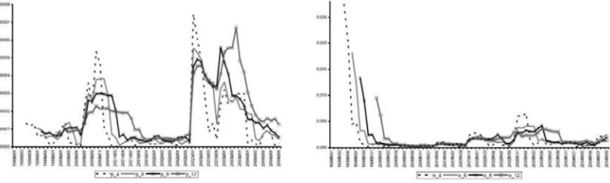
The volatilities computed by the standard deviations are presented in Graphs 2 and 3, whereE_i
andIP CA_iare the volatilities of E and IPCA, respectively, within a window of sizei. It is possible to note that the series are sensitive to the size of the window. As Table 10 shows, the unit root test forIP CA_iis also affected by window size: IP CA_4is stationary and so isIP CA_6, although we reject the presence of unit roots in the former at a level of significance of 10%. However,IP CA_8
andIP CA_12have unit roots. SinceE_iis always stationary, we computed the first differences of
IP CA_8andIP CA_12, namedd_IP CA_8andd_IP CA_12, respectively.
Figure 2 –Variances of IPCA (standard deviations from the mean) – Rolling Windows
Figure 3 – Variances of E (standard deviations from the mean) – Rolling Windows
The estimation results also are very sensitive to window size, as it can be seen in tables 11 to 14 in appendix A.9 In the four-month window, the lagged terms of a variable in its respective equation and the effect of inflation variance on exchange rate variance are considered to be statistically significant. With regard to the six-month window, there are significant cross-terms. However, the Wald test shows
8Carrera and Bastourre (2004) attribute the few macroeconomic studies about volatility to the lack of a pattern to define or
to measure volatility. According to them, the use of rolling windows, instead of subsamples, has the advantage of reducing information loss (resultant from the reduced sample size). However, this procedure is also limited due to the difficulty in determining the ideal number of observations in a window. In addition, it may imply a high correlation between the computed series, which may affect the quality of estimators, and alter the true relation between the volatilities. For instance, once the exchange rate regime varies over time, a certain window may contain two different regimes.
9The number of lags in each VAR was chosen by taking into consideration the information criteria, absence of residual
autocor-relation (LM test), absence of corautocor-relation between variables, and parsimony. In all models the dummy variabled2002_M11
– which assumes the unity value for November 2002 – was included, since in all series there is a peak in that month, proba-bly associated with the political crisis. Its inclusion allowed us to correct problems of residual autocorrelation or correlation between the variables found in the model. For similar reasons, the dummy variables d1999 in the four-month window and
that the sum of the lagged coefficients ofE_6in theIP CA_6equation is not statistically different from zero, and the same happens to the lagged coefficients ofIP CA_6 in theE_6 equation. Only the dummy and first lag of a variable are significant in the equation. In the eight-month window, only
E_8(−1)in the equation forE_8is significant, while only the dummy is significant in theD_IP CA_8
equation. However, in this VAR, the correlation betweenIP CA_8andE_8equals−0.43, which may jeopardize the OLS estimation. Finally, the VAR betweend_IP CA_12andE_12reports the coefficient ofE_12(−1)as the only significant one in theE_12equation. E_12(−1),E_12(−6)andE_12(−7)
are significant in the d_IPCA_12 equation and, according to the Wald test, their sum is statistically different from zero at a 10% level.
In sum, the relation between those two endogenous variables is sensitive to window size. De-pending on the size selected, we may accept or reject that the exchange rate variance affects inflation variance and the other way round, as well as accept or reject that lagged values of inflation variance will affect it.
4.2. Rolling Windows with variances
Once again, we have series that are very sensitive to window size, as shown in Graphs 4 and 5 (piandeiare the volatility series for IPCA and E, respectively, computed as the variance of the sample inside the window). Concerning stationarity, the only difference from the standard deviation case is that the variance of IPCA in the six-month window is not stationary (table 15 in the appendix A). Hence, we took the first difference ofp6,p8andp12, and named them asdp6,dp8anddp12, respectively.
Tables 16 to 19 in the appendix A show the results of the four estimated VARs.10 For the
four-month window VAR, only the lagged terms of each variable are significant and, differently from the previous case, the volatility of IPCA would not affect the exchange rate volatility. As for the six-month window, contrary to what was observed in the standard deviation case, the only significant terms are the dummy and the first lag of the exchange rate volatility in its own equation. In the eight-month window, we do not find the correlation problem we found before but, again, the only term that is significant ise6(−1)in the equation for the exchange rate variance. Finally, the VAR betweendp12
ande12indicatese12(−1)as the only significant variable in the equation fore12. In the equation for inflation variance, the coefficients fore12(−1)ande12(−2)are significant and the Wald test shows that their sum is statistically different from zero at a 10% level.
In sum, we notice that the results differ from the ones obtained in the case with standard deviations concerning unit root tests, the number of lags in the VAR and the significance of some variances. None of the models showed that inflation volatility is affected by its lagged term, differently from what happens to exchange rate volatility. When it comes to cross-terms, we find that exchange rate volatility is significant in explaining inflation volatility in the 12-month windows. Hence, one can realize that results are sensitive not only to window size but also to the method chosen to compute volatility. In addition, since there are lagged effects in the case of exchange rate variance, we reinforce the adequacy of investigating a GARCH-type model.
4.3. Variance decomposition in a VAR model
The last exercise performed in this section was to test a VAR between the price index and the exchange rate and to analyze variance decomposition. Since both series have unit roots, as shown in Table 1, we first tested for the presence of cointegration vectors. As shown in Table 20 in the appendix A, the Trace and Eigenvalue tests do not accept the null hypothesis of presence of a cointegration vector.11
10.D2002_M11 was included for the six-month window case
Figure 4 –Variances of IPCA (variances) – Rolling Windows
Figure 5 – Variances of E (variances) – Rolling Windows
For this reason, we will test a VAR between the first differences of price index (IPCA) and exchange rates (E).
In the variance decomposition factorization by Cholesky method, we chose E preceding IPCA, since we consider the former to be more exogenous than the latter. The Granger test may be used to give further support in the ordering decision (table 21 in the appendix A. However, since the correlation between the residuals is low(−0.17 <|0.20|)12the order does not have significant effects over the
results. Table 22 shows the VAR results, while Table 23 presents the variance decomposition.
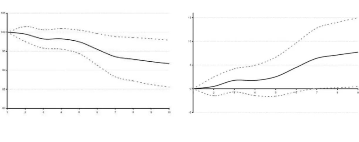
By analyzing the variance decomposition in table 23, we find that about 3% of the movements in IPCA int+ 1may be explained by shocks in E in period t. There are increasing accumulated effects over time, and shocks in E explain around 42% of the movements in IPCA after 12 months. A shock in IPCA, in its turn, does not have an immediate effect on the sequence of E, however it has lagged effects, although on a smaller scale.
Graphs 6 to 9 show these decompositions over time, as well as the interval of±2standard errors. We notice that shocks to the variables have positive effects on their sequences, and apart from the impact of IPCA on E, they are different from zero. Therefore, we cannot rule out the hypothesis that shocks to the exchange rate – represented byηtin equation 3 – might affect inflation.
Figure 6 –Percent E variance due to E Figure 7 –Percent IPCA variance due to E
12Enders (1995) suggests, as a rule-of-thumb, that a correlation between residuals of the variables<|0.2|is not strong enough
Figure 8 –Percent IPCA variance due to E Figure 9 –Percent IPCA variance due to IPCA
Based on the results presented in this section, we may infer that the traditional measures used to verify whether there is a relation between the volatilities of exchange rate and macroeconomic variables (standard deviations or variances in subsamples) yield results that are sensitive to the subsample size, leading us to accept or reject the significance of the relation according to the window size we are working with.
The variance decomposition, in its turn, indicates that shocks to the exchange rate affect inflation variance. Since volatility is also a measure of uncertainty, this result sounds more intuitive than some of those presented before: if the exchange rate affects inflation and has delayed effects (incomplete exchange rate pass-through in the short run), shocks to that variable will affect the uncertainty about future inflation. Besides, an adequate exchange rate model must consider the presence of conditional heteroskedasticity, as illustrated in Table 24 in the appendix. In this case, it is necessary to generate volatility series for both variables in the same way hence, to consider conditional variance for both -and not simply compare the variance series obtained from a GARCH(p, q)model for the exchange rates with an exogenous measure of inflation volatility. Furthermore, we show that variance decomposition reports that shocks to the IPCA affect its variance, just as well as some of the results obtained in the rolling window procedure show us that IPCA volatility is affected by its past values, reinforcing the application of the test for a bivariate GARCH model with E and IPCA.
5. TESTS WITH CONDITIONAL VARIANCE – BIVARIATE GARCH
Testing a GARCH model requires, first, some assumption about the mean equations. We considered, therefore, three different cases. The first one is consisted of only lagged terms of each variable; the second, of a Phillips Curve for the IPCA equation (according to equation 2 in Section 2) and the lagged values for the exchange rate; the third, of the Phillips Curve for the IPCA and a random walk with drift for the exchange rate (equation 3 in Section 2). According to unit root tests previously performed, both variables were considered in first differences of their logarithms. Considering both the cross-correlograms and OLS models, we chose the number of lags in the equations for IPCA and exchange rate.13 With regard to variance specifications, we tested five different options: diagonal-Vec (Bollerslev
et al., 1988), constant correlation (CCORR, from Bollerslev 1990), full parameterization (Vec), the BEKK restriction (Engle and Kroner, 1993) and the dynamic conditional correlation (DCC, from Engle 2002). Only under the BEKK restriction convergence was achieved, and we consider some reasons for that further ahead in this section.
The general form of mean, variance and covariance equations under the BEKK model are:
Mean equations
IP CA=δ0+δ1IP CAt−1+δ2Et−1+δ3Et−2+ +δ4GAPt−2+δ5P P It−1+ǫ1,t
E=γ0+γ1Et−1+γ2Et−2+ǫ2,t
Variance and Covariance equations14
h11=c11+a112 ǫ21,t−1+ 2a11a21ǫ1,t−1ǫ2,t−1+a221ǫ22,t−1+g211h11,t−1+ 2g11g21h12,t−1+g212 h22,t−1
h22=c22+a122 ǫ21,t−1+ 2a12a22ǫ1,t−1ǫ2,t−1+a222ǫ22,t−1+g212h11,t−1+ 2g12g22h12,t−1+g222 h22,t−1
h12=c21+a11a12ǫ12,t−1+ (a12a22+a21a12)ǫ1,t−1ǫ2,t−1+a21a22ǫ22,t−1 +g12g11h11,t−1+ (g11g22+g12g21)h12,t−1+g21g22h22,t−1
In order to make the analysis clearer, we renamed the coefficients above as:
c11=α0;a211=α1; 2a11a21=α2;a221=α3;g211=α4; 2g11g21=α5;g212 =α6
c22=β0;a212=β1; 2a12a22=β2;a222=β3;g122 =β4; 2g12g22=β5;g222=β6
c21=µ0;a11a12=µ1;a12a22+a21a12=µ2;a21a22=µ3;g12g11=µ4;g11g22+g12g21
=µ5;g21g22=µ6
Hence, the variance and covariance equations can be rewritten as:
h11=α0+α1ǫ21,t−1+α2ǫ1,t−1ǫ2,t−1+α3ǫ22,t−1+α4h11,t−1+α5h12,t−1+α6h22,t−1
h22=β0+β1ǫ21,t−1+β2ǫ1,t−1ǫ2,t−1+β3ǫ22,t−1+β4h11,t−1+β5h12,t−1+β6h22,t−1
h12=µ0+µ1ǫ21,t−1+µ2ǫ1,t−1ǫ2,t−1+µ3ǫ22,t−1+µ4h11,t−1+µ5h12,t−1+µ6h22,t−1
For each case, different simulations were made changing the convergence criteria and the number of iterations. Therefore, it is possible that, for each case, we ended up with more than one result achieving convergence. When this occurred, the choice was made based on the following criteria: LM and the ARCH-LM tests (i.e. absence of residual serial correlation and of arch-type residuals), calculation of the eigenvalues to assure that the condition of covariance stationarity was respected (see Engle and Kroner (1993) for further details on conditions and tests), and, when all the previous were respected, we chose the result that maximized, for the case considered, the likelihood function. The final results are presented in table 2.
By analyzing Table 2, we notice that the results for the mean equations are quite similar, as well as the values in the variance equation for cases (1) and (2). Case (3) differs from the other two but, since that model has ARCH residuals for the equation of E and serial correlation of residuals for both mean equations,15it cannot be considered as a good model.
Comparing the variance equations in cases (1) and (2), we see that the differences lie in the signs of
g12andg22, in the values ofa11,a22anda12and in the significance of coefficientsµ1,β1andβ2, that
is, the impact ofǫ2
1,t−1on the conditional variance ofE (first difference of the exchange rate) and in
the covariance and impact ofǫ2
1,t−1ǫ22,t−1on the conditional covariance ofE.
14Variance and covariance equations are from Engle and Kroner (1993), equation 2.3, pages 5 and 6, without suppressing the
GARCH terms.
15We could not find any model that removed the autocorrelation in the mean equation of the exchange rate, which was expected
Table 2 –Bivariate GARCH Results (Monthly data from 1999:01 to 2004:09)
Variables Case 1 Case 2 Case 3a Function Value 5.485.888.337 5.587.008.734 5.480.509.755
Constant 0.00282329* 0.00197323* 0.0011409*
(0.0005596) (0.00050458) (0.00051313) IP CAt−1 0.55715402* 0.57849083* 0.68315183*
(0.07376155) (0.0609667) (0.05967424) Et−1 - 0.03863824* 0.06380358*
(0.00980401) (0.00779833)
Equation for IPCA Et−2 - -0.00073484 -0.00920641
(0.00964137) (0.0073217) GAPt−2 - 0.01673604** 0.01552899**
(0.00977043) (0.0095768) P P It−1 - 0.09498593** 0.10285839*
(0.05367548) (0.05499651)
Equation for E Constant 0.00669639 0.01229489* 0.01917512*
(0.00424251) (0.0043067) (0.00534423) Et−1 0.8094822* 0.60752556*
-(0.11426506) (0.12549928)
-Et−2 -0.22750191** -0.16772685
-(0.13597143) (0.10694474)
Conditional variance of IPCA α0 0 0 0
α1 + + +
α2 + + +
α3 + + +
α4 0 0 0
α5 0 0 0
α6 0 0 0
Conditional variance of E β0 0 0 0
β1 + 0 +
β2 + 0 +
β3 + + +
β4 + + +
β5 + + +
β6 + + +
Covariance m0 + +
-µ1 - 0
-µ2 - -
-µ3 - -
-µ4 0 0 0
µ5 0 0 0
µ6 0 0 0
However, it can be seen from Table 3 that the significance ofµ1,β1andβ2is the only significant
difference between both cases. The difference in the signs ofg12andg22does not affect the final result
because these coefficients are considered under three situations: (i) squared values; (ii) multiplied by each other, (iii) multiplied by coefficients that are statistically equal to zero. The differences ina11,a22
anda12, in their turn, fall within standard deviation boundaries, thus, they may not be considered to be
significant. It is important to notice that for the inflation equation all cases provided the same signals and the same significance (i.e. if statistically equal to or different from zero). Therefore, our results for the response of IPCA to shocks in E are robust.
Table 3 –Estimated Parameters in Variance and Covariance Equations (Monthly data from 1999:01 to 2004:09)
g11 -0.1041899 -0.0513807 0.03980506*
(0.1348117) (0.11993625) (0.14292026) g21 0.00810385 0.01085598 -0.00743866*
(0.01683404) (0.01418979) (0.0156595) g12 12.52650218* -13.00132891* 13.12325566*
-155.221.793 -168.386.503 -198.208.477 g22 0.41076103** -0.43513845* 0.50120845*
(0.23448881) (0.21248228) (0.22752382) a11 0.27491257* 0.40438372* -0.44434782*
(0.12289452) (0.13130784) (0.17146475) a21 0.0595035* 0.05305404* -0.05393149*
(0.0131604) (0.01178906) (0.01283429) a12 -3.42461647** -5.71185332* 74.208.698
-198.123.913 -210.969.805 -241.134.849 a22 -0.46199166* -0.59176609* 0.78655762*
(0.1406473) (0.14044079) (0.16694871) c11 -0.00000016 -0.00000008 0.00000006
(0.007226) (0.00455714) (0.00519676) c21 0.00211834* 0.00175652* -0.00189984*
(0.00037541) (0.00033542) (0.00031271) c22 0.00366595 0.0038599 -0.00462995
(0.00836578) (0.00918004) (0.01001528) (0.00836578) (0.00918004) (0.01001528)
The Wald Test was performed to decide between the cases considered. The unrestricted case – that is, case (2) – was preferred to the detriment of cases (1) and (3), as shown in Table 4. Hence, we will consider case (2) as our results from now on.
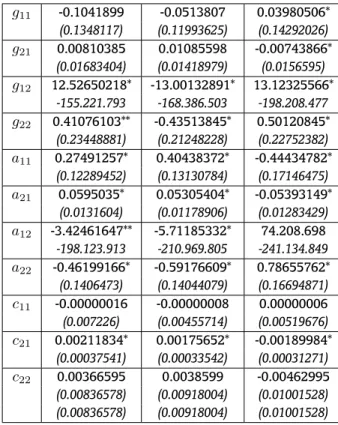
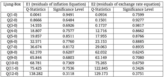
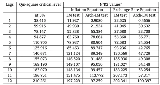
Tables 5 to 8 show the results of the Ljung-Box and LM tests for auto-correlation of residuals, the Arch-LM test for Arch-type residuals, the multivariate Portmanteau test for cross-correlation and the eigenvalue vector16 for case 2. As it can be seen from these tables, the model estimated in case 2
respects the conditions of no serial autocorrelation or cross-correlation of residuals, no Arch-type resid-uals and is covariance stationary. Therefore, we can say that the dependence between exchange rate and inflation volatilities was completely captured by the bivariate-Garch model.
By analyzing the results of case 2, shown in the second column of Table 2, one can notice that the conditional variance of IPCA is affected (statistically significant) by shocks to the IPCA, E and shocks
common to both. However, sinceα1andα3are square coefficients, we cannot determine whether the effects of IPCA and E shocks have a positive or negative sign, but we can affirm that they are statistically significant. Lagged variances and covariances, however, do not play a significant role in explaining IPCA variance.
Table 4 –Wald Testa Cases tested Observedχ2
4statistic Null hypothesis: Variables
added in case (2) are not jointly significant
Case (1) vs Case (2) 20.22 Reject
Case (2) vs.Case (3) 21.30 Reject
aWald Test:−2(lr−lu)∼χ2
q, whereqis the number of added variables,lrandluare the log-likelihood of the restricted and
unrestricted cases, respectively. UnderHo, the added variables are not jointly significant.
Table 5 –Lung-Box Tests for Residual Autocorrelation
Ljung-Box E1 (residuals of inflation Equation) E2 (residuals of exchange rate equation) Q-Statistics Significance Level Q-Statistics Significance Level
Q(1-0) 0.0041 0.9491 0.0934 0.7599
Q(2-0) 0.8666 0.6484 0.1501 0.9277
Q(3-0) 14.555 0.6926 0.1737 0.9817
Q(4-0) 18.807 0.7577 12.716 0.8662
Q(5-0) 19.857 0.8511 17.955 0.8766
Q(6-0) 32.571 0.7760 23.153 0.8885
Q(7-0) 36.674 0.8172 29.063 0.8935
Q(8-0) 62.370 0.6207 62.032 0.6245
Q(9-0) 65.844 0.6803 63.149 0.7080
Q(10-0) 68.781 0.7369 75.265 0.6750
Q(11-0) 75.425 0.7536 122.845 0.3426
Q(12-0) 138.282 0.3118 129.173 0.3751
As for the conditional variance of E, it is affected by its lagged values and by lagged values of the conditional variance of IPCA – the latter goes undetected by almost all tests with unconditional variances – although we also cannot make assertions about the sign. Shocks common to both variables
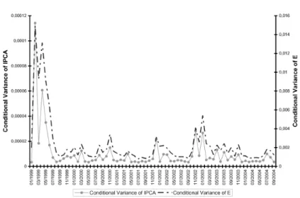
(ǫ1,t−1ǫ2,t−1)and in the covariance have a positive and significant sign. Graph 10 shows the estimated
conditional variances over time.
Finally, results show us that shocks in the exchange rate (E) and shocks common to exchange rate and IPCA have negative and significant effects over the covariance between the two variables. This is an important result in our model. It means that shocks that affect the exchange rate or the exchange rate and IPCA simultaneously will cause a “disconnection” of these two variables. After all, everything else the same, a reduction in the covariance means a reduction in the correlation coefficient between the variables.
At first, we considered that the lack of convergence for specifications other than the BEKK model would result from the small size of our sample (January, 1999 to September, 2004). However, this may be questioned since the BEKK specification has more parameters than some of the other specifications tested. The negative sign of shocks in E over the conditional covariance (µ1 < 0) and the dispersion
Table 6 –LM and ARCH-LM Tests
Lags Qui-square critical level N*R2 valuesa
Inflation Equation Exchange Rate Equation at 5% LM test Arch-LM test LM test Arch-LM test
1 38.415 11.927 0.9080 33.525 0.4656
2 59.915 49.930 21.524 41.045 30.632
3 78.147 55.838 65.384 27.580 33.708
4 94.877 62.760 78.664 53.360 36.771
5 110.705 78.937 80.904 72.583 34.554
6 125.916 85.463 89.747 93.236 42.765
7 140.671 121.124 89.349 130.569 47.729
8 155.073 146.820 91.488 185.930 49.308
9 169.190 149.107 95.050 181.027 54.148
10 183.070 148.134 99.457 183.225 53.254 11 196.751 151.475 113.772 207.173 57.317 12 210.261 197.229 97.259 202.341 100.397
aThe N*R2 value must be < than the 2 to accept the null hypotheses of no autocorrelation and arch residuals
Table 7 –Multivariate Portmanteau Test for Cross-Correlationa M Test Statistics Significance Level
3 56.954 0.3370
5 122.948 0.5036
7 165.348 0.7389
10 250.132 0.8394 12 362.776 0.6803 15 452.643 0.7660
aH
0 : ρ1 = ρ2 = · · · = ρm = 0andHa : ρi = 0for somei ∈ {1, . . . , m}(See Tsay (2002), for the multivariate
Portmanteau test for cross-correlation).
Table 8 –Eigenvalue Vector
Figure 10 –Conditional Variances – IPCA and E
variance of IPCA may not be the same all the time. If this is true, then we may have a reason for the non-convergence of specifications that, instead of working with squared terms (imposing the positivity of the matrix), try to find a sign for the relation. In these specifications, if the signs of a coefficient in the equations of exchange rate’s and inflation’s variances change from positive to negative, they will not converge to a final value, since the model will have to establish whether the coefficient is positive or negative. In the BEKK specification, however, this problem does not exist once it works with square coefficients. However, further tests are necessary before we can make such assertion.
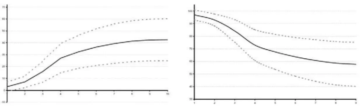
Graphs 11 to 14 are dispersion graphs with the conditional variances of E on the horizontal axis and of IPCA on the vertical axis. Graph 11 plots the entire sample and one can clearly see four outliers in that graph, which correspond to the period between February and May 1999 (i.e. the first months after the change in the exchange rate regime, caused by the 1999 crisis, and before the adoption of the inflation-targeting regime in June of that year). Hence, we excluded these observations and built Graph 12 . Again, five outliers were removed to construct Graph 13 (June 1999, November 2000, December 2001, December 2002 and January 2003). Graph 14, in its turn, was built using only the region with the highest concentration of observations (57% of the sample).17
Graph 12 and, mainly, graph 13 suggest a semiconcave (if not concave) relation between the two variables at stake (i.e. the conditional variances of exchange rate and of IPCA). To illustrate the relation, a trend was included in those graphs and in graph 14, and the adjustedR2of each trend equation was
reported (see graphs 15 to 17 in the appendix A). The semiconcave relation would imply that, although the response of inflation volatility to exchange rate volatility is positive, the proportion in its variation decreases as exchange rate volatility rises.
If we consider graph 14, which plots the region with the highest concentration of observations, we find a clear concave relation. This would mean that, after a certain point, the positive relation between volatilities becomes negative, as opposed to the convex form observed in financial variables (the so-calledsmile of volatility). Also, it is possible that it is reflecting the existence of a regime switching in the volatilities, since we are removing the extreme values of the sample. We need a longer sample to
17The observations removed from Graph 14 are, related to Graph 11: January to July 1999; November 1999 to January 2000;
test if this behavior would be reproduced over time. However, we can only use graph 14 to speculate about these possibilities happening. Nonetheless, it is a question to be answered in future research, since some works of other authors find, as we pointed out in the introduction, the sign may change according to the model’s parameters.
Figure 11 –Exchange rate and inflation volatili-ties (full sample)
0 0,00002 0,00004 0,00006 0,00008 0,0001 0,00012
0 0,002 0,004 0,006 0,008 0,01 0,012 0,014 0,016
Conditional Variance of E
C
ondi
ti
onal
Var
iance of I
P C A Graph 14 Graph 13 Graph 12
Figure 12 –Exchange rate and inflation volatili-ties (reduced sample)
0 0,000005 0,00001 0,000015 0,00002 0,000025 0,00003
0,0005 0,0015 0,0025 0,0035 0,0045 0,0055 0,0065
Conditional Variance of E
C
ondi
ti
onal
Var
iance of I
P
C
A
Graph 13
Figure 13 –Exchange rate and inflation volatili-ties (reduced sample)
0 0,000002 0,000004 0,000006 0,000008 0,00001 0,000012 0,000014
0,0005 0,001 0,0015 0,002 0,0025 0,003
Conditional Variance of E
C
ondi
ti
onal
Var
iance of I
P
C
A
Graph 14
Figure 14 –Exchange rate and inflation volatili-ties (reduced sample)
0,000003 0,0000035 0,000004 0,0000045 0,000005 0,0000055 0,000006 0,0000065
0,0007 0,0009 0,0011 0,0013 0,0015 0,0017 0,0019
Conditional Variance of E
C
ondi
ti
onal
Var
iance of I
P
C
A
6. CONCLUSIONS
The analysis presented in sections IV and V show that the use of unconditional variances leads us to results that are sensitive to the chosen measure of volatility, which is based on subjective criteria. The multivariate GARCH model, dealing directly with the effects of conditional volatilities, finds a semi-concave relation (differently from the case for financial series, where this relation has a convex form), statistically significant, between exchange rate and inflation variances.
The results seem to be in line with the intuition obtained from other studies, especially Dixit (1989) and Seabra (1996). When exchange rate volatility is very high, increasing uncertainty, inflation re-sponse may be reduced, leading to smaller effects. This may explain why some studies to placecountry-regionBrazil found a decrease in the short-run pass-through from exchange rates to consumer prices after the floating regime.
rate and inflation. The relation would exist but, under certain conditions, the disconnection between the variables would be too strong to be noticed. In periods of high volatility, agents will not respond with the same intensity as they do in periods of stability due to the lack of knowledge concerning the duration of the movements in the exchange rate (whether temporary or permanent). Therefore, inflation volatility has smaller amplitude. On the other hand, when exchange rate volatility is lower, inflation would answer more promptly.18This disconnection becomes clearer in the negative sign found
in the answer of the conditional covariance to shocks in the exchange rate and would be reinforced if the sign reversion found in graph 14 is verified in future studies.
The caveats of this paper basically lie in the small sample available for placecountry-regionBrazil, since the floating regime for exchange rates having started only in 1999. Because of that, we cannot establish with certainty whether the problems faced with convergence were due to the sign instability or to the small period involved. Nonetheless, we tend not to rely too much in the small sample expla-nation, since three out of the other four restrictions tested – diagonal VEC, CCORR and DCC – have less parameters to be estimated. Nonetheless, a large sample is essential to corroborate the results.
However, this article innovates by (i) applying a multivariate GARCH model, thus, considering con-ditional variances to analyze the relation between volatilities, (ii) trying to establish a relation between exchange rate and inflation volatilities and its possible implications for monetary policy and (iii) show-ing that traditional tests performed with exogenously constructed volatility series are sensitive to the criteria chosen to construct such series and do not reveal relevant features of that relation.
Bibliography
Andersen, T. M. (1997). Exchange rate volatility, nominal rigidities, and persistent deviations from ppp.Journal of the Japanese and International Economies, 11(4):584–609. available at❤tt♣✿✴✴✐❞❡❛s✳
r❡♣❡❝✳♦r❣✴❛✴❡❡❡✴❥❥✐❡❝♦✴✈✶✶②✶✾✾✼✐✹♣✺✽✹✲✻✵✾✳❤t♠❧.
Barkoulas, J. T., Baum, C. F., & Caglayan, M. (2002). Exchange rate effects on the volume and variability of trade flows. Journal of International Money and Finance, 21(4):481–496. available at❤tt♣✿✴✴✐❞❡❛s✳
r❡♣❡❝✳♦r❣✴❛✴❡❡❡✴❥✐♠❢✐♥✴✈✷✶②✷✵✵✷✐✹♣✹✽✶✲✹✾✻✳❤t♠❧.
Barone-Adesi, G. & Yeung, B. (1990). Price flexibility and output volatility: the case for flexible exchange rate. Journal of International Money and Finance, 9:276–298.
Barro, R. J. & Gordon, D. B. (1983). Rules, discretion and reputation in a model of monetary policy.Journal of Monetary Economics, 12(1):101–121. available at❤tt♣✿✴✴✐❞❡❛s✳r❡♣❡❝✳♦r❣✴❛✴❡❡❡✴♠♦♥❡❝♦✴
✈✶✷②✶✾✽✸✐✶♣✶✵✶✲✶✷✶✳❤t♠❧.
Baxter, M. & Stockman, A. (1988). Business cycle and the exchange rate system: some international evidence. NBER Working Papers 2689, National Bureau of Economic Research, Inc.
Bleaney, M. & Fielding, D. (2002). Exchange rate regimes, inflation and output volatility in developing countries. Journal of Development Economics, 68(1):233–245. available at❤tt♣✿✴✴✐❞❡❛s✳r❡♣❡❝✳
♦r❣✴❛✴❡❡❡✴❞❡✈❡❝♦✴✈✻✽②✷✵✵✷✐✶♣✷✸✸✲✷✹✺✳❤t♠❧.
Bleaney, M. F. (1996). Macroeconomic stability, investment and growth in developing countries.Journal of Development Economics, 48(2):461–477. available at❤tt♣✿✴✴✐❞❡❛s✳r❡♣❡❝✳♦r❣✴❛✴❡❡❡✴❞❡✈❡❝♦✴
✈✹✽②✶✾✾✻✐✷♣✹✻✶✲✹✼✼✳❤t♠❧.
18For instance, in an environment with fixed exchange rates, the agents know that devaluation is permanent. Therefore, facing
Bollerslev, T. (1990). Modelling the coherence in short-run nominal exchange rates: A multivariate generalized arch model. The Review of Economics and Statistics, 72(3):498–505. available at❤tt♣✿
✴✴✐❞❡❛s✳r❡♣❡❝✳♦r❣✴❛✴t♣r✴r❡st❛t✴✈✼✷②✶✾✾✵✐✸♣✹✾✽✲✺✵✺✳❤t♠❧.
Bollerslev, T., Engle, R. F., & Wooldridge, J. M. (1988). A capital asset pricing model with time-varying covariances. Journal of Political Economy, 96(1):116–31. available at❤tt♣✿✴✴✐❞❡❛s✳r❡♣❡❝✳♦r❣✴❛✴
✉❝♣✴❥♣♦❧❡❝✴✈✾✻②✶✾✽✽✐✶♣✶✶✻✲✸✶✳❤t♠❧.
Calvo, G. A. & Reinhart, C. M. (2000a). Fear of floating. NBER Working Papers 7993, National Bureau of Economic Research, Inc. available at❤tt♣✿✴✴✐❞❡❛s✳r❡♣❡❝✳♦r❣✴♣✴♥❜r✴♥❜❡r✇♦✴✼✾✾✸✳❤t♠❧.
Calvo, G. A. & Reinhart, C. M. (2000b). Fixing for your life. NBER Working Papers 8006, National Bureau of Economic Research, Inc. available at❤tt♣✿✴✴✐❞❡❛s✳r❡♣❡❝✳♦r❣✴♣✴♥❜r✴♥❜❡r✇♦✴✽✵✵✻✳❤t♠❧.
Carrera, J. & Bastourre, D. (2004). Could the exchange rate regime reduce macroeconomic volatility? In
Econometric Society 2004: Latin American Meetings (LAMES). Econometric Society. available at❤tt♣✿
✴✴✐❞❡❛s✳r❡♣❡❝✳♦r❣✴♣✴❡❝♠✴❧❛t♠✵✹✴✸✵✾✳❤t♠❧.
Chen, N. (2004). The behaviour of relative prices in the european union: A sectoral analysis. European Economic Review, 48:1257–1286.
Devereux, M. B. & Engel, C. (2003). Monetary policy in the open economy revisited: Price setting and exchange-rate flexibility. Review of Economic Studies, 70(4):765–783. available at❤tt♣✿✴✴✐❞❡❛s✳
r❡♣❡❝✳♦r❣✴❛✴❜❧❛✴r❡st✉❞✴✈✼✵②✷✵✵✸✐✹♣✼✻✺✲✼✽✸✳❤t♠❧.
Dixit, A. K. (1989). Hysteresis, import penetration, and exchange rate pass-through. The Quarterly Journal of Economics, 104(2):205–28. available at ❤tt♣✿✴✴✐❞❡❛s✳r❡♣❡❝✳♦r❣✴❛✴t♣r✴q❥❡❝♦♥✴
✈✶✵✹②✶✾✽✾✐✷♣✷✵✺✲✷✽✳❤t♠❧.
Duarte, M. & Stockman, A. (2002). Comment on: Exchange rate pass-through, exchange rate volatility, and exchange rate disconnect.Journal of Monetary Economics, 49(5):941–946.
Enders, W. (1995).Applied econometric time serie. John Wiley & Sons, Nova York.
Engel, C. & Rogers, J. H. (2001). Deviations from purchasing power parity: causes and welfare costs.
Journal of International Economics, 55(1):29–57. available at❤tt♣✿✴✴✐❞❡❛s✳r❡♣❡❝✳♦r❣✴❛✴❡❡❡✴
✐♥❡❝♦♥✴✈✺✺②✷✵✵✶✐✶♣✷✾✲✺✼✳❤t♠❧.
Engle, R. (2002). Dynamic conditional correlation: A simple class of multivariate generalized autore-gressive conditional heteroskedasticity models.Journal of Business & Economic Statistics, 20(3):339–50. available at❤tt♣✿✴✴✐❞❡❛s✳r❡♣❡❝✳♦r❣✴❛✴❜❡s✴❥♥❧❜❡s✴✈✷✵②✷✵✵✷✐✸♣✸✸✾✲✺✵✳❤t♠❧.
Engle, R. F. & Kroner, K. F. (1993). Multivariate simultaneous generalized arch. Economics Working Paper Series 89-57r, Department of Economics, University of California at San Diego. available at
❤tt♣✿✴✴✐❞❡❛s✳r❡♣❡❝✳♦r❣✴♣✴❝❞❧✴✉❝s❞❡❝✴✽✾✲✺✼r✳❤t♠❧.
Flood, R. P. & Rose, A. K. (1995). Fixing exchange rates a virtual quest for fundamentals. Jour-nal of Monetary Economics, 36(1):3–37. available at❤tt♣✿✴✴✐❞❡❛s✳r❡♣❡❝✳♦r❣✴❛✴❡❡❡✴♠♦♥❡❝♦✴
✈✸✻②✶✾✾✺✐✶♣✸✲✸✼✳❤t♠❧.
Ghosh, A. R., Gulde, A.-M., Ostry, J. D., & Wolf, H. C. (1997). Does the nominal exchange rate regime matter? NBER Working Papers 5874, National Bureau of Economic Research, Inc. available at❤tt♣✿
Hausmann, R., Panizza, U., & Stein, E. (2001). Why do countries float the way they float? Journal of Development Economics, 66(2):387–414. available at❤tt♣✿✴✴✐❞❡❛s✳r❡♣❡❝✳♦r❣✴❛✴❡❡❡✴❞❡✈❡❝♦✴
✈✻✻②✷✵✵✶✐✷♣✸✽✼✲✹✶✹✳❤t♠❧.
Krugman, P. (1988).Exchange Rate Instability. The MIT press, Cambridge, MA.
Obstfeld, M. & Rogoff, K. (2000). The six major puzzles in international macroeconomics: Is there a common cause? NBER Working Papers 7777, National Bureau of Economic Research, Inc. available at
❤tt♣✿✴✴✐❞❡❛s✳r❡♣❡❝✳♦r❣✴♣✴♥❜r✴♥❜❡r✇♦✴✼✼✼✼✳❤t♠❧.
Rogoff, K. (2001). Perspectives on exchange rate volatility. In Feldstein, M., editor,International Capital Flows, pages 441–453. University of Chicago Press.
Seabra, F. (1996). A relação teórica entre incerteza cambial e investimento: os modelos neoclássico e de investimento irreversível.Política e Planejamento Econômico, 26(2):183–202.
Smith, C. E. (1999). Exchange rate variation, commodity price variation and the implications for international trade. Journal of International Money and Finance, 18(3):471–491. available at http://ideas.repec.org/a/eee/jimfin/v18y1999i3p471-491.html.
Sutherland, A. (2005). Incomplete pass-through and the welfare effects of exchange rate variability. Journal of International Economics, 65(2):375–399. available at http://ideas.repec.org/a/eee/inecon/v65y2005i2p375-399.html.
Tsay, R. S. (2002).Analysis of Financial Time Series. John Wiley & Sons, Inc.
Wei, S.-J. & Parsley, D. C. (1995). Purchasing power disparity during the floating rate period: Exchange rate volatility, trade barriers and other culprits. NBER Working Papers 5032, National Bureau of Economic Research, Inc. available at❤tt♣✿✴✴✐❞❡❛s✳r❡♣❡❝✳♦r❣✴♣✴♥❜r✴♥❜❡r✇♦✴✺✵✸✷✳❤t♠❧.
A. TABLES & GRAPHS
Table 9 –ADF Unit Root Test
sample: 2000:03 to 2004:10
Variable ADF test statis-tics
Critical value at 5%
ADF test statis-tics – first differ-ence of the vari-able
Critical value at 5%
Price Index -2.1704 (a) -34.783 -3.904127(a) -34.783 Exchange Rate -1.7097 (a) -34.783 -7.427513(a) -34.783 External Prices -1.5419 (a) -34.783 -8.014687(a) -34.793
GAP -97.018 -29.077 -
Table 10 –ADF Unit Root Test – std. dev.
sample: 2000:03 to 2004:10
Variable ADF test statis-tics
Critical Value at 5%
ADF test statis-tics first differ-ence of variables
Critical Value at 5%
IPCA_4 -34.697 -34.805 -
-IPCA_6 -1.8540(a) -19.461 -
-IPCA_8 -1.3046 (a) -19.463 -70.015 -34.865
IPCA_12 -0.8823(a) -19.465 -59.875 -34.921
E_4 -119.597 -34.816 -
-E_6 -10.8574 (b) -29.084 -
-E_8 -9.5054(b) -29.100 -
-E_12 -7.5521(b) -29.136 -
-Note: test performed with (a) trend or intercept and (b) without trend.
Table 11 –VAR for four-month windows
Variables E_4 IPCA_4 Variables E_4 IPCA_4 E_4(-1) 0.2790 -5.65E-05 D2002_M11 0.005 7.11E-05
(0.0449) (0.0004) (0.001) (8.7E-06) [6.2085] [-0.1423] [5.1319] [ 8.1232] IPCA_4(-1) 21.8600 0.7206 D1999 0.0121 1.59E-06 (7.7321) (0.0683) (0.0015) (1.4E-05) [2.8272] [10.5446] [7.8898] [0.1177] C 0.0004 2.27E-06 R-squared 0.8856 0.7384
(0.0002) (1.4E-06) Adj. R-squared 0.8779 0.7210 [2.2992] [1.5965] F-statistic 116.0581 42.3377
Table 12 –VAR for six-month windows
Variables E_6 IPCA_6 Variables E_6 IPCA_6 Variables E_6 IPCA_6
E_6(-1) 0.9027 0.0034 E_6(-6) 0.0706 -0.0010 IPCA_6(-5) -265.070 -0.0059
(0.1118) (0.0018) (0.0482) (0.0008) (7.8289) (0.1248)
[ 8.0747] [ 1.9157] [1.4657] [-1.343] [-3.3858] [-0.0469]
E_6(-2) 0.0398 -0.0064 IPCA_6(-1) 0.4882 0.8246 IPCA_6(-6) 19.6540 -0.0141
(0.1483) (0.0024) (7.085) (0.1129) (6.1560) (0.0981)
[0.2684] [-2.7097] [0.0689] [7.3032] [ 3.1927] [-0.1434]
E_6(-3) 0.0239 -0.0002 IPCA_6(-2) 1.8361 0.1457 C 0.0002 1.86E-06
(0.1548) (0.0025) (9.0902 (0.1449) (0.0001)
(1.8E-06)
[ 0.1546] [-0.0727] [ 0.202] [ 1.0061] [ 1.8206] [ 1.0462
E_6(-4) -0.1345 0.0043 IPCA_6(-3) -43.719 -0.0721 D2002_M11 0.0028 4.59E-05
(0.1139) (0.0018) (8.7652) (0.1397) (0.0004)
(6.8E-06)
[-1.1809] [ 2.3814] [-0.4989] [-0.5159] [ 6.5062] [ 6.7698]
E_6(-5) -0.1018 0.0005 IPCA_6(-4) 7.9487 -0.0954 R-squared 0.88102 0.8588
(0.0874) (0.0019) (8.6463) (0.1378) F-statistic 25.0626 20.5897
[-1.1643] [ 0.3891] [ 0.9193] [-0.6920] Adj.
R-squared
0.8459 0.8171
Table 13 –VAR for eight-month windows
Variables E_8 D_IPCA_8 Variables E_8 D_IPCA_8 E_8(-1) 0.7930 0.0016 D_IPCA_8(-2) 53.804 -0.04323
(0.0987) (0.001) -91.884 (0.0900) [ 8.0398] [ 1.6026] [ 0.5856] [-0.4790] E_8(-2) 0.0097 -0.0006 C 0.0002 -1.79E-06 (0.0674) (0.0007) (0.0001) (1.1E-06) [ 0.1439] [-0.9426] [ 1.8207] [-1.63756] D_IPCA_8(-1) 18.755 0.09867 D2002_M11 0.0015 4.21E-05
Table 14 –VAR for twelve-month windows
Variables E_12 D_IPCA_12 Variables E_12 D_IPCA_12 Variables E_12 D_IPCA_12
E_12(-1) 11.266 0.0066 E_12(-7) -0.01345 0.00166 D_IPCA_12(-6) 695.244 -0.0856
(0.1548) (0.0017) (0.0727) (0.0008) -81.141 (0.0874)
[ 7.2795] [ 3.9409] [-0.1849] [ 2.1149] [ 0.8568] [-0.9788]
E_12(-2) -0.0864 -0.0041 D_IPCA_12(-1) -73.151 0.1543 D_IPCA_12(-7) -81.538 0.0164
(0.2702) (0.0029) -99.846 (0.1076) -76.083 (0.082)
[-0.3197] [-1.394] [-0.7326] [ 1.4338] [-1.0717] [ 0.2005]
E_12(-3) -0.15121 0.0009 D_IPCA_12(-2) 53.827 0.107 C 8.75E-05 -1.55E-06
(0.2749) (0.003) -98.458 (0.1061) (9.6E-05) (1.0E-06)
[-0.5499] [ 0.3009] [ 0.5467] [ 1.0081] [ 0.9099] [-1.4988]
E_12(-4) 0.1970 -0.0028 D_IPCA_12(-3) -118.497 -0.0342 D2002_M11 -0.000391 2.64E-05
(0.2605) (0.0028) -105.016 (0.1132) (0.0003) (3.7E-06)
[ 0.7565] [-0.9924] [-1.12837] [-0.3018] [-1.1375] [ 7.1275]
E_12(-5) -0.1114 0.0021 D_IPCA_12(-4) -0.5193 -0.1149 D2003_M10 -0.0018 1.46E-05
(0.2391) (0.0026) -101.884 (0.1098) (0.0004) (3.8E-06)
[-0.466] [ 0.7939] [-0.051] [-1.0465] [-5.0760] [ 3.8268]
E_12(-6) 0.0218 -0.0040 D_IPCA_12(-5) 142.164 0.0848 R-squared 0.9317 0.8543
(0.1654) (0.0018) -92.135 (0.0993) Adj. R-squared 0.8986 0.7837
[ 0.1315] [-2.2462] [ 1.543] [ 0.8540] F-statistic 281.265 120.931
Table 15 –ADF Unit Root Test – variances
sample: 2000:03 to 2004:10
Variable ADF test statis-tics
Critical Value at 5%
ADF test statis-tics first differ-ence of variables
Critical Value at 5%
p4 -3.2566(b) -29.069 -
-p6 -2.5156 (b) -29.084 -73.599 -3.484
p8 -0.8460 (a) -19.463 -73.398 -34.865
p12 -0.4167 (a) -19.467 -59.193 -34.922
e4 -65.715 -34.816 -
-e6 -5.8641 (b) -29.084 -
-e8 -5.4361 (b) -29.100 -
-e12 -4.5351 (b) -29.136 -
-Note: test performed with (a) trend or intercept and (b) without trend
Table 16 –VAR for four-month windows
Variable E4 p4 Variables E4 p4
E4(-1) 0.6525 0.002503 C 0.0088 0.0008 (0.0605) (0.00665) (0.0032) (0.0004) [ 10.7898] [ 0.37628] [ 2.7471] [ 2.1113] P4(-1) 0.0791 0.700972 R-squared 0.6643 0.4998
(0.8394) (0.09233) Adj. R-squared 0.6534 0.4837 [ 0.0942] [ 7.59224] F-statistic 613.330 30.976
Table 17 –VAR for six-month windows
Variable E6 dp6 Variable E6 dp6
e6(-1) 0.7630 0.0083 Dp6(-1) 0.7124 0.0221 (0.1127) (0.0136) (0.8625) (0.1044) [ 6.7736] [ 0.6068] [ 0.826] [ 0.2116] e6(-2) 0.0101 -0.0126 Dp6(-2) 0.43334 -0.1202
(0.0903) (0.0109) (0.8515) (0.1031) [ 0.1113] [-1.1549] [ 0.509] [-1.1664] C 0.0064 3.82E-05 D2002_M11 0.02998 0.0056
(0.0024) (0.0003) (0.0077) (0.0009) [ 2.6605] [ 0.1319] [ 3.8767] [ 6.0109] R-squared 0.7255 0.4332 Adj. R-squared 0.7006 0.3817 F-statistic 290.747 84.069
Table 18 –VAR for eight-month windows
Variable E8 dp8 Variables E8 dp8
e8(-1) 0.8994 0.0203 dp8(-1) 0.0669 0.0222 (0.1177) (0.0151) -10.564 (0.1351) [ 7.6418] [ 1.3501] [ 0.0633] [ 0.1639] e8(-2) -0.0595 -0.0136 dp8(-2) 0.1905 -0.007
(0.0988) (0.0126) -10.548 (0.1349) [-0.6021] [-1.0740] [ 0.1806] [-0.0512] C 0.0052 -0.0002 R-squared 0.7267 0.0338
(0.0025) (0.0003) Adj. R-squared 0.7064 -0.0378 [ 2.0663] [-0.6696] F-statistic 358.896 0.4722
Table 19 –VAR for twelve-month windows
Variables E12 dp12 Variables E12 dp12 Variables E12 dp12
e12(-1) 0.9752 0.0413 dp12(-1) -0.9046 0.1774 C 0.0028 -0.0004
(0.1086) (0.0124) -11.596 (0.1325) (0.0023) (0.0003)
[8.976] [3.3225] [-0.7802] [1.3391] [1.2268] [-1.5782]
e12(-2) -0.0543 -0.0290 dp12(-2) -0.1943 0.17707
R-squared
0.8348 0.245
(0.1014) (0.0116) -11.187 (0.1278) Adj.
R-squared
0.8216 0.1846
[-0.5357] [-2.5057] [-0.1736] [1.3851]
F-statistic
Table 20 –Cointegration test between exchange rate and consumer price index
Trend assumption: Linear deterministic trend
Series: ln (exchange rates) and ln (consumer price index); Lag interval (in first differences): 1 to 4 Unrestricted Cointegration Rank Test (Trace)
Number of coin-tegration vectors underH0
Eigenvalue Trace statistic Critical Value (5%)
p-value **
None 0.1048 8.3109 15.495 0.4328
At most one 0.019 1.2275 3.8412 0.2679
Unrestricted Cointegration Rank Test (Maximum Eigenvalue) Number of
coin-tegration vectors under Ho
Eigenvalue Trace statistic Critical Value (5%)
p-value **
None 0.1048 7.0834 14.2646 0.4793
At most one 0.019 1.2275 3.8415 0.2679
** MacKinnon-Haug-Michelis (1999) p-values
Table 21 –Granger Causality Testa
Null Hypothesis Number of Obs. F-statistic p-value E does not Granger-Cause IPCA 66 9.0601 5.0E-05 IPCA does not Granger-Cause E 1.4686 0.2323
Table 22 –VAR between E and IPCA
Variables E IPCA Variables E IPCA
E(-1) 0.6036 0.0356 IPCA(-1) 0.9185 0.6556
(0.1217) (0.0111) -12.735 (0.1163)
[4.9597] [3.201] [0.7213] [5.6392]
E(-2) -0.1168 -0.0037 IPCA(-2) -2.704 -0.2059
(0.1501) (0.0137) -15.498 (0.1415)
[-0.7780] [-0.2669] [-1.7447] [-1.4555]
E(-3) 0.1183 0.0220 IPCA(-3) 24.593 0.1452
(0.1239) (0.0113) -15.498 (0.1415)
[0.9547] [1.9463] [1.5868] [1.0260]
E(-4) 0.0827 -0.0051 IPCA(-4) -25.399 0.06289
(0.1033) (0.0094) -11.504 (0.1050)
[0.8007] [-0.5394] [-2.2079] [0.5988]
C 0.01652 0.0018 D2002_M11 -0.135 0.0143
(0.0084) (0.0008) (0.0344) (0.0031)
[1.9756] [2.3730] [-3.9256] [4.5682]
R-squared 0.4582 0.7168 Adj.
R-squared
0.3696 0.6704
F-statistic 51.688 154.665
Note: Std. deviations in parenthesis and t-statistics in square brackets.
Table 23 –Variance Decomposition (Cholesky ordering: place E IPCA)
Variance decomposition of E: Variance decomposition of IPCA: Period Std. Error E IPCA Period Std. Error E IPCA
Table 24 –OLS Equation for E
Variable Coefficient Standard Error t-statistic p-value
C 0.0059 0.0092 0.6378 0.5258
AR(1) 0.4341 0.0964 45.041 0.0000 R2 0.2351 LM Test (1 lag) (a) 0.8708 Adjusted R2 0.2235 ARCH-LM Test (1 lag) 28.6673 (b)
Note: (a) null hypothesis of absence of autocorrelation accepted also for higher number of lags; (b) null hypothesis of absence of ARCH residuals rejected at 1%.
Figure 15 –Exchange rate and inflation volatili-ties (reduced sample)
y = -0.372x2 + 0.0064x - 3E-06
Adjusted R2
= 0.6915 0 0,000005 0,00001 0,000015 0,00002 0,000025 0,00003
0,0005 0,0015 0,0025 0,0035 0,0045 0,0055 0,0065
Conditional Variance of E
C
ondi
ti
onal
Var
iance of I
P
C
A
Graph A.2
Figure 16 –Exchange rate and inflation volatili-ties (reduced sample)
y = -1.1874x2 + 0.0073x - 2E-06
adjusted R2
= 0.4842 0 0,000002 0,000004 0,000006 0,000008 0,00001 0,000012 0,000014
0,0005 0,001 0,0015 0,002 0,0025 0,003
Conditional Variance of E
C
ondi
ti
onal
Var
iance of E
Graph A.3
Figure 17 –Exchange rate and inflation volatilities (reduced sample)
y = -4.2952x2 + 0.0114x - 3E-06
Adjusted R2= 0.1339
0,000003 0,0000035 0,000004 0,0000045 0,000005 0,0000055 0,000006 0,0000065
0,0007 0,0009 0,0011 0,0013 0,0015 0,0017 0,0019 Conditional Variance of E
C
ondi
ti
onal
Var
iance of I
P
C
B. DIAGNOSTIC TESTS FOR THE BI-GARCH MODEL
This appendix brings a brief explanation about the test of covariance stationarity in the multivariate Garch model under the BEKK restriction. For details, see Engle and Kroner (1993).
In a bivariate GARCH (1,1), the conditional variance has the form:
u211t
u212t
u2 22t = c11 c12 c22 +
B11 B12 B13
B21 B22 B23
B31 B32 B33
σ11(2 t−1) σ2
12(t−1)
σ2 22(t−1)
+
A11 A12 A13
A21 A22 A23
A31 A32 A33
u211(t−1) u2
12(t−1)
u2 22(t−1)
Without exogenous variables, the BEKK restriction has the form:
Ut=C∗
′
1 C1∗+
B∗
11 B12∗
B∗
21 B22∗
′
σ12,t−1 σ1,t−1σ2,t−1
σ2,t−1σ1,t−1 σ22,t−1
B∗
11 B12∗
B∗
21 B22∗
+
A∗
11 A∗12
A∗
21 A∗22
′
[Ut−1]
A∗
11 A∗12
A∗
21 A∗22
To assure the process is covariance stationary, the eigenvalues of
q
i=1
K
k=1
(B∗
ik⊗Bik∗)+ p
i=1
K
k=1
(Aik⊗
Aik)must be minor than the unity, in absolute values. In other words, we have to calculate the
eigen-value of matrix X below:
X =
(a11∗a11) + (g11∗g11) (a11∗a12) + (g11∗g12) (a12∗a11) + (g12∗g11) (a12∗a12) + (g12∗g12) (a21∗a11) + (g21∗g11) (a11∗a22) + (g11∗g12) (a12∗a21) + (g12∗g21) (g12∗g22) + (g12∗g21) (a21∗a11) + (g21∗g11) (a21∗a12) + (g21∗g12) (a22∗a11) + (g22∗g11) (a22∗a12) + (g2∗g12) (a21∗a21) + (g21∗g21) (a21∗a22) + (g21∗g22) (a21∗a22) + (g21∗g22) (a22∗a22) + (g22∗g22)
Calculating the eigenvalues of X using the coefficients for case 2 presented in table 3 along the text, we find the following vector y of eigenvalues:
y= 0.6630 -0.4252 -0.0770 0.0637