A Clustering Approach for Vehicle Routing Problems with Hard Time Windows

(1)

Sergejs Pugacs Master Thesis

A Clustering Approach for Vehicle Routing Problems

with Hard Time Windows

Dissertação para obtenção do Grau de Mestre em Logica Computicional

Orientador : Professor Pedro Barahona, CENTRIA, Universidade Nova de Lisboa

Júri:

Presidente: Doutor José Júlio Alves Alferes, Professor Catedrático da Faculdade de Ciências e

Tecnologia da Universidade Nova de Lisboa

Arguente: Doutor Enrico Franconi, Associate Professor, Free University of Bozen-Bolzano

Vogal: Doutor Pedro Manuel Corrêa Calvente de Barahona, Professor Catedrático da

(2)

A Clustering Approach for Vehicle Routing Problems with Hard Time Windows

Copyright cSergejs Pugacs, Faculdade de Ciências e Tecnologia, Universidade Nova de Lisboa

(3)

Acknowledgements

(4)

Abstract

The Vehicle Routing Problem (VRP) is a well known combinatorial optimization problem and many studies have been dedicated to it over the years since solving the VRP optimally or near-optimally for very large size problems has many practical applications (e.g. in various logistics systems). Vehicle Routing Problem with hard Time Windows (VRPTW) is probably the most studied variant of the VRP problem and the presence of time windows requires complex techniques to handle it. In fact, finding a feasible solution to the VRPTW when the number of vehicles is fixed is an NP-complete problem. However, VRPTW is well studied and many different approaches to solve it have been developed over the years.

Due to the inherent complexity of the underlying problem VRPTW is NP-Hard. Therefore, optimally solving problems with no more than one hundred requests is considered intractably hard. For this reason the literature is full with inexact methods that use metaheuristics, local search and hybrid approaches which are capable of producing high quality solutions within practical time limits.

In this work we are interested in applying clustering techniques to VRPTW problem. The idea of clustering has been successfully applied to the basic VRP problem. However very little work has yet been done in using clustering in the VRPTW variant. We present a novel approach based on clustering, that any VRPTW solver can adapt, by running a preprocessing stage before attempting to solve the problem.

(5)

Resumo

O Problema de Roteamento de Veículos (VRP) é um problema de otimização combinatória bem conhecido e objecto de muitos estudos ao longo dos anos, desde a resolução óptima de VRPs ou à resolução aproximada para grandes problemas de tamanho tem muitas aplicações práticas (por exemplo, em vários sistemas de logística). Problemas de roteamento de veículos com janelas temporais (VRPTW) é provavelmente a variante mais estudada do problema VRP em que a presença de janelas de tempo requer técnicas complexas para a sua resolução. De facto, encontrar uma solução viável para o VRTPTW quando o número de veículos está fixado é um problema NP-completo. No entanto,o VRTPTW está bem estudado e muitas abordagens diferentes para resolvê-lo foram desenvolvidas ao longo dos anos.

Devido à sua complexidade inerente o problema VRPTW é NP-Difícil. Portanto, resolver de forma otimizada problemas com mais de cerca de uma centena de pedidos é considerada intratável difícil. Por isso, a literatura está plena de métodos que usam metaheurísticas inexactas, pesquisa local e abordagens híbridas, capazes de produzir soluções de alta qualidade em tempos razoáveis.

Neste trabalho estamos interessados em aplicar técnicas de agrupamento para o problema VRPTW. A idéia de agrupamento tem sido aplicado com sucesso para o problema básico VRP. No entanto, muito pouco tem sido feito ainda no uso de agrupamento na variante VRPTW. Nesta dissertação, é apresentada uma nova abordagem baseada em agrupamento, que qualquer resolvedor VRPTW pode adaptar, executando uma etapa de pré-processamento antes de se tentar resolver o problema.

(6)

List of Figures

2.1 Example of savings heuristic. Two routes〈i−2,i−1,i,〉and〈j,j+1,j+2,〉merged

into a single route〈i−2,i−1,i,j,j+1,j+2〉. . . 10

2.2 Example of a 2-opt move . . . 11

2.3 Example of a Or-opt move. . . 12

3.1 Request distance visualization in both space and time . . . 20

3.2 Waiting time dependence on the departure time . . . 21

3.3 Constant servicing time within interval[b_i,l_i] . . . 22

3.4 Second macro node is before the first macro node. . . 25

3.5 Second macro node is after the first macro node . . . 25

3.6 Earliest arrival of the second macro node is after the earliest departure of the first macro node. . . 27

3.7 Earliest arrivalE_k′of the new combined macro node. . . 28

3.8 Early arrival of second macro node before the early departure of first macro node. . 28

3.9 Latest arrival of second macro node is before the latest departure of the first macro node 29 3.10 Latest arrivalL_k′of the new combined macro node. . . 30

3.11 Latest arrival of the second macro node request is after the latest departure of the first 30 4.1 Example of neighborhood without any merge options. . . 37

4.2 Ilustration of the distance heuristic between two macro node requests . . . 38

4.3 Ilustration of the waiting time heuristic between two macro node requests . . . 39

4.4 Ilustration of the flexibility cost between two macro node requests . . . 40

5.1 Mean number of vehicles needed by class . . . 44

5.2 Relative performance of different combinations . . . 45

(10)

LIST OF FIGURES x

5.4 Route duration broken down by class . . . 48

5.5 Execution time broken down by class . . . 49

5.6 Reduction rate broken down by class . . . 50

5.7 Characteristic metrics forα=0.1,β=1.0,γ=1.0 . . . 51

5.8 Reduction rate forα=0.1,β=1.0,γ=1.0 . . . 52

5.9 Characteristic metrics forα=0.1,β=1.0,γ=1.0 for 10k instances. . . 53

(11)

1

Introduction

1.1 Introduction

Logistics is the management of the flow of goods between the point of origin and the point of consumption in order to meet some requirements set by the customers or companies. Any institution that performs any kind of large scale deliveries faces the problems of deciding how, what and when to deliver to minimize their costs. Even though the problem can be traced back to ancient civilizations, only with the appearance of digital computers, this problem could be solved automatically.

Modern day logistics systems have to handle problems of servicing thousands or even tens of thousands requests. And the problem becomes even harder when the logistics systems have to take into account external constraints that have to be respected in order to fulfill the request.

The Vehicle Routing Problem (VRP) is the core problem in these systems. It is a well known combinatorial optimization problem and many studies have been dedicated to it over the years. The problem was first formalized by[7]. Therefore solving the VRP optimally or near-optimally for very large size problems has many practical applications.

Due to the inherent complexity of the underlying problem VRP is NP-Hard. Therefore, optimally solving problems with no more than one hundred requests is considered intractably hard[22,1], due to the inherent complexity of the problem. For this reason the literature is full with inexact methods that use metaheuristics, local search and hybrid approaches which are capable of producing high quality solutions within practical time limits.

(12)

1. Introduction 1.1. Introduction

be serviced in a particular time period. VRPTW is probably the most studied variant of the VRP problem and it can be considered the primary ‘rich‘ variant because the presence of time windows require complicated techniques for constant time feasibility checks.[27]has shown that, even, finding a feasible solution to the VRPTW when the number of vehicles is fixed is a NP-complete problem. However, VRPTW is well studied and many different approaches to solve it have been developed over the years. Recent advances have been presented in[13].

In this work we are interested in applying clustering techniques to VRPTW problem. The idea of clustering has been successfully applied to the basic VRP problem[14]. However very little work has yet been done in using clustering in the VRPTW variant.

Our proposed algorithm uses the clustering idea to identify a set of nearby requests that can be replaced by a single macro request. This process is repeated and the set of requests is eventually replaced by a set of macro node requests. The new problem, consisting of macro nodes, is much smaller and a solver can find a solution for this problem much faster. The cost of this speed-up is the error that is introduced by treating clusters as single node requests. The hypothesis that we want to verify, is whether the error introduced by clustering is small enough and is worth the benefits in the speedup.

To test this hypothesis, we implement our proposed clustering algorithm and numerically evaluate it on the benchmark set[12]. In addition, we use the benchmark set to construct new larger problems, to see if the clustering works with very large problems.

(13)

2

State of Art

2.1 Preliminaries

The goal of this section is to introduce a unified notation, that can be used unambiguously throughout all of the work.

2.1.1 Formal Problem Definition

The VRPTW can be formally stated as the problem of designingleast cost routesfrom a depotDto a set of requestsRusing a homogeneous fleet of vehiclesV. Each requestr ∈Ris associated with a demandq_r≥0 and a service times_r≥0. The travel cost between request r_i andr_j is denoted byt_{i j}. In addition each request r is associated with a interval[e_r,l_r]that represents its service time

window. The request r must be serviced within this time interval. Specifically e_r represents the earliest service time for requestr andl_r represents the latest service time for requestr. A vehicle may arrive earlier thane_r but it has to wait until timee_r to be begin servicing the request.

Finally, all feasible vehicle routes start and end at the depot, while the quantities to deliver up to any request of a route must not exceed the vehicle capacityQ. The vehicles leave the depot at timee_o, at the earliest and must return to the depot by timel_o, at the latest.

2.1.2 Objective Function

(14)

2. State of Art 2.2. Exact Methods

requests are served and all constraints imposed by vehicle capacity, service times and time windows are satisfied.

The presented formulation of VRPTW is an established model and many different approaches have been proposed and successfully employed to solve it. Broadly these approaches can be divided into two separate groups

1. Exact methods

2. Heuristic methods

2.2 Exact Methods

Exact algorithms for VRPTW are based on Integer Linear Programming (ILP). Integer Linear Pro-gramming is a Linear ProPro-gramming (LP) technique were the domains of all of the variables are restricted to be integers. Linear Programming is a technique for the optimization of a linear objective function, subject to linear equality and linear inequality constraints. Its feasible region is a convex polyhedron, which is a set defined as the intersection of finitely many half spaces, each of which is defined by a linear inequality. Its objective function is a real-valued affine function defined on this polyhedron. A linear programming algorithm finds a point in the polyhedron where this function has the smallest (or largest) value if such a point exists.

The general form of a Linear Programming formulation looks like

maximizecTx subject toAx≤b

andx≥0

2.2.1 Integer Programming formulation of the VRPTW

LetN={1,...,n}be the set of requests. In addition 0 andn+1 represent the starting and ending

node for all paths, which in our case is a single depo location. LetK, indexed byk, be the set of available vehicles to be routed and scheduled. Consider the graphG= (V,A), where the set of nodes

is equal toV =N∪ {0,n+1}, and the setAcontains all feasible arcs, that isA⊆V×V. For each requesti∈N, there is a known quantityq_i, a time window[e_i,l_i]and a service times_i. We assume that all vehicles are empty in the depot thereforeq₀₍_k₎=0 for each vehiclek∈K. Every vehiclekhas a working time interval[Ek_,_Lk_]_{, that we express by associating a time window with nodes 0 and}

n+1,[e₀₍_k₎,l₀₍_k₎] = [e_n₊₁₍_k₎,l_n₊₁₍_k₎] = [Ek,Lk].

(15)

not exceeded.

We present a Integer Programming formulation involving three types of variables: flow variables X_{i j}k,(i,j)∈A,k∈K, equal to 1 if arc(i,j)is used by vehiclekand 0 otherwise; time variablesT_ik,i∈ V,k∈K specifying the start of service at nodei by vehiclek; and load variablesLk

i,i∈V,k∈K

specifying the load of the vehiclekafter servicing nodei.

(VRPTW) min X

k∈K

X

(i,j)∈A

c_{i j}X_{i j}k (2.1)

subject to

X

k∈K

X

j∈N∪{n+1}

X_{i j}k =1 ∀i∈N (2.2)

X

k∈K

X

j∈N

X_0,k_j ≤v (2.3)

X

j∈N∪{n+1}

X₀k_j =1 ∀k∈K (2.4)

X

i∈N∪{0}

X_{i j}k − X i∈N∪{n+1}

X_{j i}k =0 ∀k∈K,∀j ∈N (2.5)

X

i∈N∪{0}

X_ik_,_n₊₁=1 ∀k∈K (2.6)

X_{i j}k(T_ik+s_i+t_{i j}k −T_jk)≤0 ∀k∈K,(i,j)∈A (2.7)

e_i≤T_ik≤l_i ∀k∈K,∀i∈V (2.8)

X_{i j}k(Lk_i +q_i−Lk_j) =0 ∀k∈K,(i,j)∈A (2.9)

Lk_i ≤Qk ∀k∈K,∀i∈N∪ {n+1} (2.10)

Lk₀=0 ∀k∈K (2.11)

X_{i j}k ≥0 ∀k∈K,(i,j)∈A (2.12)

X_{i j}k ∈ {0,1} ∀k∈K,(i,j)∈A (2.13)

The objective function (2.1) of this nonlinear formulation expresses the total cost. It is possible to add a fixed costcof using a vehicle by addingc_0,_j,j∈N, then to minimize the number of vehicleschas to be selected large enough to be greater than any route total distance. Given thatN=V \ {0,n+1}

represents the set of customers, constraint2.2restricts the assignment of each customer to exactly one vehicle route. Constraints2.4-2.6characterize the flow on the path to be followed by vehiclek. Constraints2.7-2.8guarantee schedule feasibility with respect to time considerations and2.9-2.11

ensure feasibility of capacity aspects. Constraint2.13makes the condition variables binary.

(16)

relaxation.

2.2.2 Column Generation

The main idea in Column Generation is that many linear programs are too large to consider all the variables explicitly. Since most of the variables will be non-basic and assume a value of zero in the optimal solution, only a subset of variables need to be considered in theory when solving the problem. Column generation leverages this idea to generate only the variables which have the potential to improve the objective function.

The problem being solved is split into two problems: the master problem and the subproblem. The master problem is the original problem with only a subset of variables being considered. The subproblem is a new problem created to identify a new variable. The objective function of the subproblem is the reduced cost of the new variable with respect to the current dual variables, and the constraints require that the variable obey the naturally occurring constraints.

2.2.3 Dantzig Method

The Dantzig-Wolfe decomposition is a special case of the Delayed Column Generation process and works by identifying which of the constraints are connected. Constraints are connected if the same variable appears in both of them. The method separates the global list of constraints into buckets such that only connected constraints appears in each bucket. In addition the objective function is simplified for each bucket to contain only those variables that are present in the constraints.

Each bucket then forms a subproblem. The solution for each subproblem gives rise to a set of points that represent the feasible region of this subproblem. The solution to the master problem must lie somewhere on the intersection of all this feasible regions. Therefore the solution to the master problem, cab be expressed as a convex combination of the points forming the feasible regions of the subproblems.

The essence of the Dantzig-Wolfe decomposition is to construct the master problem that tries to minimize the objective function by finding a convex combination of the points from the polyhedron formed by the intersection of all the polyhedra formed by the individual subproblems.

More formally, given that each subproblem has a feasible region that forms a convex polyhedron represented by a set of pointsX_i=<x₁,...,x_n>, the polyhedron formed by the intersection of all polyhedra is equal to ˆX =Tm_i₌₁X_i. And the set of points that represent this polyhedron is equal to

ˆ

X =<y₁,...,y_k>. We can formulate the objective function of the master problem using this set.

The objective function becomes a linear combinationΛof the points ˆX.

(17)

subject to

Ax≤b

x≥0

Λ≥0

X

i=1

λ_i=1 λ_i∈Λ

2.2.3.1 Dantzig-Wolfe Method with Integer Linear Programming

The Dantzig-Wolfe method was originally designed to work with Linear Programming and not Integer Linear Programming. However under certain assumptions we can still apply it to ILP. The conditions for application must be that the solution of the linear relaxation (LP) of the Integer Programming model must be equal to the original Integer Programming model. This property is called the integrality property.

Since we can not solve any ILP models directly we first linearize them and solve the linear versions using standard Simplex algorithms for solving LP. But we must have the guarantee that the linear solutions are transferable to the integer models.

2.2.3.2 Dantzig-Wolfe decomposition of the VRPTW

Here we give an example one can use to define the subproblem. We can decompose the original problem based on the observation that it consists of|K|disjoint subproblems, one for each vehi-cle. Then each subproblem becomes that of finding an elementary shortest path with time and capacity constraints. Consequently, the flow variablesX_{i j}k can be expressed as a nonnegative convex combination of the paths generated from the subproblems.

In the case of VRPTW, the linearized subproblem does not posses the integrality property. But it can still be solved as a nonlinear integer program. The elementary shortest path problem with capacity and time constraints is known to beN P-hard. However if we allow nonelementary path solutions, i.e. solutions where a path may contain cycles of finite duration, pseudo-polynomial algorithms exist.

2.2.4 Lagrangian Relaxation Method

(18)

2.2.4.1 Mathematical Description

Given a linear programming model s.t. x∈RnandA∈Rm,n.

maximizecTx subject to

Ax≤b

We can separate the constraints inAinto two partsA₁∈Rm1,nandA₂∈Rm2,n. We can then write

the original problem as.

maximizecTx subject to

A₁x≤b

A₂x≤b

Then we can apply the main idea of the Lagrangian method of introducing some of the constraints inside the objective value. And assigning nonnegative weightsλ = (λ₁,...,λ_m₂)to penalize the

objective value for violating the constraints.

maximizecTx+λ(b₂−A₂x)

subject to

A₁x≤b

λ≥0

Therefore it is always the case that the optimal result to the Lagrangian Relaxation problem will be no smaller than the optimal result to the original problem.

2.2.4.2 Lagrangian relaxation for VRPTW

(19)

2. State of Art 2.3. Heuristics

2.2.5 Numerical Results

For the single depot VRPTW with a homogeneous fleet the Dantzig-Wolfe decomposition found optimal solutions to a number of 100-customer problems[8]. Later it was improved by[20]. This work added 2-path inequalities to linear relaxation of the subproblem formulation.

In[19]presented a Branch and Bound (BB) algorithm were the relaxation was computed using the Lagrangian Relaxation. These methods were based on 2-cycle elimination algorithms. Later [16]described a BB algorithm where the pricing subproblem is solved with a k-cycle elimination procedure.

The results show that the Dantzig-Wolfe decomposition performs much better then the Lagrangian relaxation methods. Not only did the Dantzig-Wolfe method solve more problems, it did so in with less computational time used.

2.3 Heuristics

Given the inherent computational difficulty of the VRPTW, a variety of heuristics have been reported in the literature that achieve sub-optimal solutions.

We divide heuristics into the following categories:

1. Insertion Heuristics

2. Improvment Heuristics

3. Metaheuristics

Heuristics are often used because they provide a tractable way of tackling NP-Hard problems. Even though they do not provide a guarantee of finding the best solution, often their solutions are good enough. Additionally, heuristics are often simple to describe and implement, which leads to their easy adaptability to many VRP variants.

2.3.1 Insertion Heuristics

Insertion heuristics build a feasible solution by inserting at every iteration an unrouted customer into a partial route. This process is performed either sequentially, one route at a time, or in parallel, where several routes are considered simultaneously. The process has to decide two things, which unrouted customer to insert and where to insert it. Usually the algorithms use metrics based on distance, waiting time and savings to answer these questions.

2.3.1.1 Clarke and Wright savings algorithm

(20)

tries to minimize the number of vehicles used.

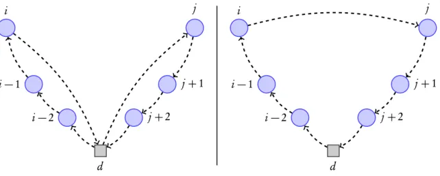
It is based on the notion ofsavings. Initially, the solution consists ofn back and forth routes between the depo and each customer. Then during every iteration, two routes(d,...,c_i,d)and (d,c_j,...,d)are merged into a single route(d,...,c_i,c_j,...,d)whenever that is feasible. This merge

then generates a saving ofs_{i j}=c_{i d}+c_{d j}−c_{i j}. See Figure2.1for an example.

d i−2

i−1 i

j+2

j+1

j

d i−2

i−1 i

j+2

j+1

j

Figure 2.1: Example of savings heuristic. Two routes〈i−2,i−1,i,〉and〈j,j+1,j+2,〉merged

into a single route〈i−2,i−1,i,j,j+1,j+2〉.

Solomon in[29]reports a variant of the CW algorithm in which savings are adapted to handle time windows, but results are disappointing.

2.3.1.2 Solomon

Sequential insertion heuristics for the VRP with time windows were first proposed by [29]. It proposed a two-criteria insertion algorithms. The first criteria assigns all unrouted customers their best feasible insertion position based on distance and waiting time. And the second criteria selects the best candidate based on the savings concept.

Formally, letc₁(i,u,j)andc₂(i,u,j)be the first and the second criteria to insert customer u between two adjacent customersiand j. Then for each unrouted customeru we compute its best feasible insertion cost as

c₁(i(u),u,j(u)) = min

ρ=1,...,mc1(iρ−1,u,iρ)

After selection the insertion position, then the customer to be selected is chosen by the second criteria as

c₂(i(u∗),u∗,j(u∗)) =max

(21)

2.3.2 Improvement Heuristics

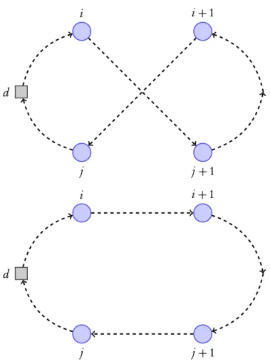
Route improvement heuristics start with a feasible solution and then in each iteration try to improve it. This is done by exploring a neighborhood of possible candidate solutions. Generally, a neighborhood is the set of solutions that can be reached from the present one by swapping a subset ofr arcs between solutions. An arc exchange is applied only if it improves the objective function. Arc improvement heuristics are classified by the number or arcs they interchange - 2-Opt, 3-Opt, and in generalk-Opt. Or by the type of operation that the exchange performs - Or-Opt. In the case of Or-Opt, there is not need to reverse any route segments.

2.3.2.1 2-Opt

First presented in[6]for solving the traveling salesman problem.

d

i i+1

j j+1

d

i i+1

j j+1

Figure 2.2: Example of a 2-opt move

(22)

2.3.2.2 Or-Opt

There is a problem with the 2-opt heuristic, in that it requires one to reverse the customer order. An alternative approach proposed by[23]consists of generating only those moves that do not require customer reordering. The idea is to relocate a chain of consecutive customers. This is achieved by replacing three edges in the original tour by three new ones without modifying the orientation of the route as shown in the Figure2.3

d

i−1

j+1

i+1 i

i+2

j

d

i−1

j+1

i+1 i

i+2

j

Figure 2.3: Example of a Or-opt move.

2.3.3 Metaheuristics

A metaheuristic is an iterative generation process which guides and subordinates heuristics by com-bining intelligently different concepts for exploring and exploiting the search space, while learning strategies are used to structure information in order to find efficient near-optimal solutions[24].

Metaheuristics are the core of recent work on approximation methods for the VRPTW, and they mainly include Simulated Annealing (SA) and Tabu Search (TS).

(23)

2. State of Art 2.4. Clustering and Decomposition Approaches in VRPTW

2.3.3.1 Tabu Search

Tabu search was first proposed in[15]. The main idea is to avoid looping in cycles by forbidding or penalizing moves which return states that were already previously visited. Thus a heuristic that is driven by TS may end up accepting a solution of lower quality and making a degrading move, in order to escape visiting states that were previously explored. This insures that new regions of problem solution space will be explored in the goal of avoiding local minima.

[11]were the first to adapt the TS metaheuristic to the VRPTW problem. Their approach consisted of using the Solomon’s insertion heuristic to produce an inital solution and then post-optimize it with both 2-opt and Or-opt.

2.3.3.2 Simulated Annealing

Simulated Annealing (SA) is a probabilistic metaheuristic first described by[18]where a modification to the current solution that leads to an increase in solution cost can be accepted with some probability. This mechanism allows the method to escape from bad local optima.

At each step, the SA heuristic considers some neighbouring state s′of the current states, and probabilistically decides between moving the system to states′or staying in states. The probability of making this transition is specified by anacceptance functionthat depends on the objective values of statess ands′beingE(s)andE(s′)respectively, and on a global time-varying parameter T called the

temperature. As the temperature decreases the probability that the acceptance function will make a degrading move must decrease as well. Therefore it is usual to model the acceptance function as

p(s,s′,T) =e−(E(s)−E(s

′₎₎

T

SA has been successfully applied to the VRPTW by[4].

2.4 Clustering and Decomposition Approaches in VRPTW

In the previous sections we have described the general and historically well studied methods for solving VRP with time windows. In this part we present those methods that demonstrate the idea of clustering to help solve VRPTWs.

2.4.1 Cluster-First and Route-Second

(24)

2. State of Art 2.4. Clustering and Decomposition Approaches in VRPTW

2.4.2 Gillett 1974

[14]are the first authors adopting the cluster-first and route-second method to solve VRPs. They developed a sweep-based heuristic in which customers are partitioned into different groups according to their polar coordinates as well as the vehicle capacity. A TSP is then solved in each group.

However, in the case for the VRPTW, it usually fails to construct a feasible route in the second stage due to the required service time window. [29]extended this VRP algorithm to VRPTW by repeating thecluster-first and route-secondprocedure with all unscheduled customers until the problem is solved.

2.4.3 Fisher 1981

[10]proposed a two-phase algorithm for vehicle routing: in the first phase, it finds an assignment of customers to vehicle routes, and then continued by a route improvement procedure. A number of seed customers are selected by some criteria, and then the cost from each non-seed customer to each seed customer is calculated by the additional distance when the non-seed customer is inserted between the seed customer and the depot.

2.4.4 Dondo 2007

[9]proposed a three stage hybrid approach. During stage 1 requests are combined into clusters. Then, during stage 2, a new problem is solved based on the combined clusters and the remaining unclustered requests, using an exact MILP solver. After, as stage 3, for each route a separate TSP optimization is run to find the best order of visits within this route.

Work proposed by Dondo is very similar to our approach, it also tries to construct clusters in order to reduce the size of the problem, however it then uses an exact solver to route the clusters into complete routes.

The difference between our work and Dondo is in the way Dondo creates clusters. First, Dondos cluster construction is parameterized by the two parameters

(a) the maximum distance between two nodes inside the cluster

(b) the maximum waiting time between two nodes inside the cluster.

In this way the process implicitly controls the reduction size, by only allowing clusters with the given properties. These numbers have to be manually selected depending on the structure of the problem. Instead, our approach is explicitly controlled by setting the desired reduction size.

The second difference, is that Dondo only allows to insert an unrouted request into the current cluster, however we are more flexible and allow for merges between any two clusters.

(25)

2. State of Art 2.5. Indigo

fulfills the parameters a) and b). We, on the other, propose a heuristic function based on distance, waiting time and time window flexibility.

Since Dondo uses an exact solver, it is only able to solve problems up to 100 requests. Therefore we can not directly compare the results of Dondo with our approach.

2.4.5 Qi 2012

[25]proposed a method to partition the customers into clusters that jointly considers the spatial and temporal information. It represents time and space in the same coordination system, and develops a method to measure the space-temporal distance between two customers. However the method considers the soft version of the time window problem, where a violation of time windows does not invalidate a solution, but just penalize the objective function value.

2.4.6 Savelsbergh 1985

[27]was the first to suggest that information about a route can be summarized by a so calledmacro nodein a few parameters, that allowed to decide if a new request can be inserted into the route in constant time instead of recomputing time feasibility constraints.

2.4.7 Bent 2010

Another way to speed-up neighborhood search algorithms is to perform decoupling in an effort to define sub-problems that can be optimized independently and then reinserted into an existing solution.

[2] proposed a so-called randomized adaptive spatial decoupling (RAND). RAND considers spatial decoupling and produces independent feasible sub-problems. A further improvement was later proposed in[3]. Where decoupling of the subproblem was based on spacial, temporal and space-temporal properties of customer requests. These approaches have been successfully applied on large-scale VRPTW instances.

Similarly, spatial decoupling acceleration techniques have been also utilized by[21].

2.5 Indigo

Although many techniques are presented in the literature, there are no publicly available implemen-tations that one can use to compare performances of these techniques, since most of Operations Research work is done by either private companies or private research laboratories. However the authors of this work had access to the VRPTW solverIndigodeveloped at NICTA1.

We briefly present the Indigo solver and show that this solver is comparable with other state of the art solutions.[17]presents the architecture as well as the benchmark results of the Indigo solver.

(26)

2. State of Art 2.5. Indigo

2.5.1 Solver Architecture

Indigo builds the solution in two phases. During phase one, a feasible solution is constructed using the Clarke’s savings method and during phase two a local search algorithm is used to improve on the solution.

The improvement phase uses the Large Neighborhood Search (LNS) metaheuristic. Indigo internally uses a Constraint Programming (CP) framework to model the problem as a variable assignment problem. Combining this CP representation allows Indigo to effectively prune large sections of the unfeasible search space.

Using CP as the underlying model allows Indigo to be very flexible in modeling the side constraints of the classical VRP. One can easily extend indigo to handle much more expressive VRP variants.

2.5.2 Benchmarks

According to[17]in 2011, Indigo was able to improve the results of the benchmark data set in[12], namely, to find new best results for 83 out of 300 benchmarks.

Bellow in Table2.1, we show performance as a ratio between Indigo’s result and the best know results reported in the literature.Sizegives the number of customers in the problem;Bestgives the number of problems where a new best was found;Meanis the mean increase;80%gives the 80th percentile of increase; andMaxgives the maximum increase over best-known solution. For example, 1.02 means that Indigo results were 2% worse than the best-known solution.

Size Best Mean 80% Max

200 11 1.01 1.02 1.05

400 13 1.01 1.03 1.06

600 19 1.02 1.04 1.10

800 18 1.02 1.05 1.11

1000 22 1.03 1.06 1.14

(27)

3

Macro Nodes

The final goal of this work is to speed up VRPTW solvers by encoding a problem instance into one that is smaller in size and, therefore, much faster to solve. The new instance is constructed in such a way, that the solution of the new instance can be translated back to the solution of the original instance.

To perform this reduction in size, we identify sets of requests that can be replaced by a single request. Since the new instance has several requests replaced by a single request it is smaller in size. This new instance is then solved with the state of the art solver Indigo. The solution of the new instance that is obtained with Indigo can then be translated back to the solution of the original larger instance.

The task then is to find sets of requests that can be replaced by a single request. The new request which would replace this set acts like amacro node. This new request must characterize servicing of the whole set. Nevertheless the macro node must be represented as a single VRPTW request.

In this chapter we show how starting with individual requests one can combine them into larger macro nodes and how to represent such macro nodes by an abstraction of single requests.

3.1 Macro Nodes

(28)

3. Macro Nodes 3.1. Macro Nodes

can be passed to Indigo as a proper VRPTW problem.

A VRPTW problem description consists of the following data:

• A set of requests

• Description of the vehicle fleet

Since we do not do anything that affects the vehicle fleet, this part of the problem specification is just passed over to Indigo as is. However, we change the request set by reducing its size and introducing new requests.

We repeat what exactly constitutes a request. A requestr is defined by the following properties:

• Its geographic locationp_r where the service is to take place.

• Its demand quantity denoted byq_r.

• Its servicing time window interval denoted by[e_r,l_r].

• Its servicing time durations_r.

More formally a request can be defined as a tuple with 5 components.

Definition 1. A request r is defined by a tuple〈e_r,l_r,s_r,q_r,p_r〉, where e_r and l_r are the earliest and latest arrival times, s_r is the servicing time, p_r is the geographic location and q_r is the demand quantity of the request r .

Therefore, any macro node object that is constructed must be replaceable by a single request with the listed properties. This fact puts a limitation on what kind of macro node objects we are be able to construct.

3.1.1 Structure of the macro nodes

As already stated, the goal of the macro node object is to replace several requests by a single request. This single request must have a fixed location, a fixed servicing time window interval, a fixed demand quantity and a fixed servicing time duration.

In order to simplify the mapping of a macro node to a single request, the proposed algorithm assumes that the order in which we visit requests in the macro node is fixed at macro node construction time. This assumption makes the structure of a macro node object not a set like object, but instead a sequence like object, where the sequence determines the visit order of the requests inside the macro node. Committing to a fixed visit order inside the macro node gives us an easier way to replace a set of requests by a single request. Therefore servicing a macro nodes automatically determines the order of servicing all the requests inside the macro node.

Now that we gave the intuition of what a macro node object represents, we can give a formal definition.

(29)

3. Macro Nodes 3.2. Macro Node Request

3.2 Macro Node Request

Given that a macro node is a sequence of requests that have to be serviced and given that the servicing of this macro node must be mapped to servicing of a single new request, we introduce the concept of amacro node request. The properties of the macro node request are computed in such a way, that if a feasible solution of a VRPTW problem contains a macro node request then replacing this macro node request with the actual sequence of requests of the macro node would not make this solution unfeasible.

Definition 3. If m_k=〈r₁,...,r_n〉is a macro node then this macro node can be represented by amacro node requestr_m

k. Where rmk is a tuple

r_m_k =〈E_k,L_k,S_k,Q_k,p_{f i r s t}_k,p_{l as t}_k〉

Arrival at the request r₁within the time windows[E_k,L_k]will make it feasible to service all requests in the macro node m_k, the servicing time S_kshould be equivalent in duration to servicing all the requests in m_kand traveling between the requests and, also, waiting if necessary, and the demand quantity Q_k has to represent the total demand for the whole macro node. The locations p_{f i r s t}

k and pl as tk are the locations of the first request of the macro node and the location of the last request of the macro node.

Therefore themacro node requestr_m_k is a single request with a feasible arrival interval[E_k,L_k]

a servicing timeS_kand demand quantityQ_k. But instead of a single location as in the case of a request, a macro node request has two locations - a starting location p_{f i r s t}

k and a finishing location pl as tk.

The above definition does not specify how to compute the valuesE_k,L_k,S_kandQ_kgiven a macro nodem_k. The remaining part of this section is dedicated to the problem of computing these values.

3.3 Macro Node Visualization

Before continuing to explain additional properties of macro nodes, we introduce our request visu-alization technique. The purpose of this visuvisu-alization technique is to show the proximity of two requests in time and space simultaneously.

(30)

3. Macro Nodes 3.4. Servicing time of a Macro Node Request

Time Distance

e_i l_i

e_j l_j

b_i

b_j

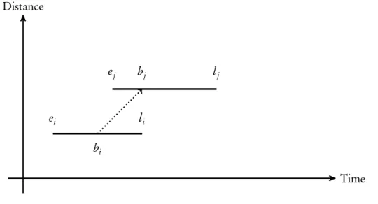
Figure 3.1: Request distance visualization in both space and time

Figure3.1shows two requestsiand j, with their corresponding time window intervals[e_i,l_i]

and[e_j,l_j]respectively. Also, it shows a departure from requestiat timeb_i and an arrival at request j at timeb_j.

3.4 Servicing time of a Macro Node Request

Servicing a macro node entails servicing all the requests in this macro node. We can decompose this servicing time into three components.

• Time spent traveling between all requests of the macro node.

• Minimal time spent waiting for the feasible interval to become active.

• Time spent servicing individual requests.

Definition 4. If m_k =〈r₁,...,r_n〉is a macro node and r_m

k =〈Ek,Lk,Sk,Qk,pf i r s tk,pl as tk〉is its macro node request then the value S_kis equal to

S_k= n

X

i=1

s_i+ n−1

X

i=1

t_i_,_i₊₁+ n

X

i=2

w_i

where w_iis the minimal waiting time incured before request r_i.

(31)

3. Macro Nodes 3.4. Servicing time of a Macro Node Request

Figure3.2illustrates the different waiting times between two requests.

Time Distance

e_i l_i

e_j l_j

w_j

Figure 3.2: Waiting time dependence on the departure time

In Figure3.2departing from the requestr_iat timee_i+s_iwould lead to some waiting timew_j, but departing at timel_i+s_iwould lead to no waiting time. Therefore the total servicing time of both requests depends on what time we start servicing the first request, since we might or might not incur some waiting time in between the requests. This means the total servicing time is a function on the start time of the two requests.

This leads to a problem, since if we want to represent a macro node as a single request it must have a fixed total servicing time. To overcome this dependency on the starting time, the resulting macro node requests, that represent servicing all of their requests, should have a time window that always ensures a fixed minimal total servicing time.

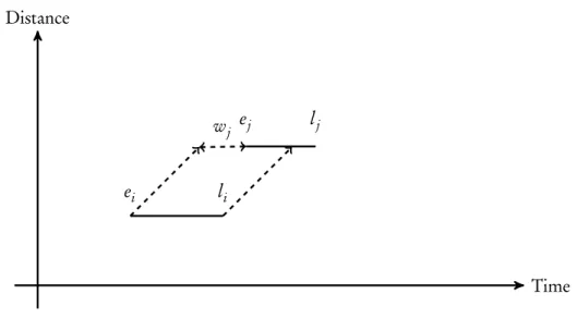
As shown in Figure3.3, for the example that we have just given, if we restrict the time window of the resulting macro node request to the interval[b_i,l_i]then the overall servicing time of this macro

(32)

3. Macro Nodes 3.5. Demand quantity of a Macro Node Request

Time Distance

e_i l_i

e_j l_j

b_i

Figure 3.3: Constant servicing time within interval[b_i,l_i]

3.5 Demand quantity of a Macro Node Request

Computing demand quantity of a macro node request is simple to compute, since for a fixed macro node the total demand of this macro node is always the sum of the demands of individual requests.

Definition 5. If m_k =〈r₁,...,r_n〉is a macro node then the demand quantity Q_k of the macro node request r_m

k =〈Ek,Lk,Sk,Qk,pf i r s tk,pl as tk〉of mk is equal to

Q_k= n

X

i=1

q_i

3.6 Distance between Macro Node Requests

We already mentioned that each requestr is associated with a geographic location p_r. And for every pair of requestsr_i andr_j the distance between them is defined as:

t_p_i_,_p_j

Since Euclidean distance is a symmetric property it is equal in both ways

t_p

i,pj =tpj,pi

(33)

3. Macro Nodes 3.7. Constructing Macro Nodes

To encode a macro node as a single request one has to find a way to encode the geographical distance between macro nodes. Since a macro node is just a sequence of requests one can represent the distance to a macro node as the distance to the first request of this macro node. In the same way, the distance from a macro node to other objects can be measured as the distance from the last request of this macro node. Formally we define it as:

Definition 6. If r_m

k =〈Ek,Lk,Sk,Qk,pf i r s tk,pl as tk〉and rml =〈El,Ll,Sl,Ql,pf i r s tl,pl as tl〉 are two macro node requests, then the distance between these two requests is computed as :

t_k′_,_l =t_p

l as tk,pf i r s tl t_l′_,_k=t_p

l as tl,pf i r s tk

Now the distance between two macro node requests is the distance between the location of the last request in the macro nodem_k and the location of the first request in the macro nodem_l and vice versa.

Also, for all macro node requestsr_m

k the distance from the macro node request to itself is 0.

t_k′_,_k=0

3.7 Constructing Macro Nodes

We start the macro node creation process by creating a macro nodem_k of size 1 for every request k∈R. The properties of the macro node requestr_m_k of this macro nodem_k are equal to the original requestk.

E_k=e_k

L_k=l_k

S_k=s_k

Q_k=q_k

p_{f i r s t} k =pk p_{l as t}

K =pk

(34)

the requests in both macro nodes. Next we show how to compute the properties of the new macro node request after combining two macro nodes.

3.7.1 Joining two Macro Nodes

In future visualizations instead of displaying all the request sequence of a macro node, we depict the macro node by drawing its macro node request. This simplification does not remove any important details since the time window of the macro node request adequately characterizes it, and more so allows to simplify the visualizations.

There are three distinct cases of joining two macro nodes. We examine each case separately and show how to decide if the two macro nodes can be combined and, whenever possible, what is the resulting macro node request that characterizes servicing both macro nodes.

The three cases are based on the temporal relationship between the two macro nodes we are considering to combine together. To avoid repetition, we analyze all cases by considering two macro node requestsr_m_k =〈E_k,L_k,S_k,Q_k,p_{f i r s t}_k,p_{l as t}_k〉andr_m_l =〈E_l,L_l,S_l,Q_l,p_{f i r s t}_l,p_{l as t}_l〉to form a combined macro node requestr_m

k′=〈Ek′,Lk′,Sk′,Qk′,pf i r s tk′,pl as tk′〉

3.7.2 Case one - unfeasible clustering

As the first case we consider the situation where the earliest departure timeE_k+S_kof the first macro node requestr_m

k =〈Ek,Lk,Sk,Qk,pf i r s tk,pl as tk〉plus the travel timet

′

k,l to reach the macro node

requestr_m_l =〈E_l,L_l,S_l,Q_l,p_{f i r s t}_l,p_{l as t}_l〉exceeds the latest arrivalL_l. Formally we can state this condition as:

E_k+S_k+t_k′_,_l >L_l

(35)

Time Distance

E_k L_k

E_l L_l Ek+Sk+t_k′_,_l

Figure 3.4: Second macro node is before the first macro node

Whenever two macro nodes fulfill this condition, combining them is impossible.

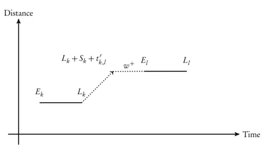
3.7.3 Case two - clustering with extra waiting time

In our second case, we consider the temporal situation when the earliest arrival of the second macro node requestE_l is later then the latest departureL_k+S_kplus travel timet_{k l}′ between the macro node requests. Formally we write this condition as:

L_k+S_k+t_k′_,_l <E_l

Figure3.5illustrates case two.

Time Distance

w+

E_k L_k

E_l L_l

L_k+S_k+t_k′_,_l

(36)

In this case, even if we service the first macro node as late as possible at timeL_kthen we will still incur a waiting time costw+_{between macro nodes}_m

k andml.

To guarantee that the waiting time between the macro node requests is minimal, the first macro node request must be started as late as possible. Hence, the result of combining r_m_k = 〈E_k,L_k,S_k,Q_k,p_{f i r s t}

k,pl as tk〉and rml =〈El,Ll,Sl,Ql,pf i r s tl,pl as tl〉is equal to the macro node r_m

k′=〈Ek′,Lk′,Sk′,Qk′,pf i r s tk′,pl as tk′〉, where the properties of rm′k are defined as follows:

E_k′=L_k

L_k′=L_k

S_k′=S_k+S_l+w++t_k′_,_l

Q_k′=Q_k+Q_l

p_{f i r s t}

k′ =pf i s tk p_{l as t}

k′ =pl as tl

In fact, to guarantee minimal waiting time, the time window of the new macro node request collapsed to the interval[L_k,L_k], that is a single point interval. The motivation for collapsing the

time window of the combined request is as following. The vehicle always has to wait the waiting timew+_{. However, starting to service the macro node}_m

kat some time earlier thanLkwould only

cause additional waiting time to be added to the unavoidable waiting timew+_{. Collapsing the time}

window leads to an overall smallest total waiting time spent inside the macro node.

3.7.4 Case three - clustering with overlapping time windows

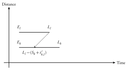
Case one analyzed a second macro node before the first one. Case two analyzed a second macro node well after the first one. Case three is the remaining case, when there is some overlap between the macro node request time windows. Therefore the condition of case three can be defined as the negation of the condition of cases one and two. Negation of the condition of case one is that the latest arrival time of the second macro node request must be greater or equal to the earliest departure time plus the travel time of the first macro node request. Formally it can be written as:

L_l ≥E_k+S_k+t_k′_,_l

The negation of the condition of case two would be that the earliest arrival of the second macro node request is earlier then the latest departure plus travel time of the first macro node request. Formally we write that as:

(37)

To show the result of combining two macro nodes, we further distinguish four different cases. Two cases of temporal relationship between the earliest arrival times of both macro nodes and two cases of temporal relationship between the latest arrival times of both macro nodes.

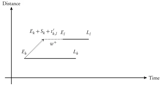
3.7.4.1 New earliest arrival time

Let us consider case 3.1 where the earliest arrival time of the second macro node requestE_l is later than the earliest departure time of the first macro nodeE_k+S_k plus the travel time between the nodest_k′_,_l. Formally this condition can we written as:

E_l >E_k+S_k+t_k′_,_l

Figure3.6demonstrates the relationship between the early arrival times of both macro nodes.

Time Distance

w+

E_k L_k

E_l L_l

E_k+S_k+t_k′_,_l

Figure 3.6: Earliest arrival of the second macro node is after the earliest departure of the first macro node

In order to avoid introducing extra waiting timew+, which will result in a longer overall ser-vicing time of the combined macro node, we will push forward the earliest arrival timeE_k to avoid introducing the waiting timew+_.

To avoid the waiting time between the two macro nodes the earliest arrival time of the combined macro node request is equal to

E_k′=E_l−(S_k+t_k′_,_l)

(38)

Time Distance

E_k L_k

E_l L_l

E_l −(S_k+t_k′_,_l)

Figure 3.7: Earliest arrivalE_k′of the new combined macro node

The other case (case 3.2) of the relationship of earliest arrival time between the two macro nodes is when the earliest arrival time of the second macro node is earlier than the earliest departure time of the first macro node plus the travel time between them. Formally we write it as:

E_l ≤E_k+S_k+t_k′_,_l

See Figure3.8for an illustration of the time relationship in case 3.2.

Time Distance

E_k L_k

E_l Ek+Sk+t_k′_,_l L_l

Figure 3.8: Early arrival of second macro node before the early departure of first macro node

(39)

be narrowed, and the earliest arrival time of the combined macro node stays the same as the earliest arrival time of the first macro node.

E_k′=E_k

Cases 3.1 and 3.2 can be handled by a single formulation

E_k′=max(E_k, E_l−(S_k+t_k_,_l))

3.7.4.2 New latest arrival time

Similarly, we also have two cases for the relationship between the latest arrival time of the two macro node requests.

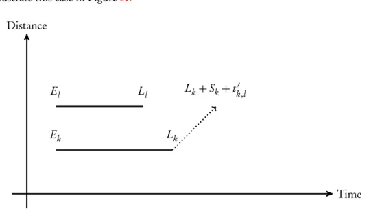
In case 3.3 the latest arrival time of the second macro node requestL_l is earlier than the latest departure time of the first macro node requestL_k+S_kplus the travel time betweent_k′_,_l. Formally it can be written as:

L_l <L_k+S_k+t_k′_,_l

We illustrate this case in Figure3.9

Time Distance

E_k L_k

E_l L_l Lk+Sk+t_k′_,_l

Figure 3.9: Latest arrival of second macro node is before the latest departure of the first macro node

Servicing the first macro node request at its latest arrival timeL_kwould make it impossible to service the second macro node within its time window[E_l,L_l]. Therefore the combined macro node

request has to narrow its latest arrival time such that both macro node requests can be feasible. The value of the latest arrival time of the combined macro node request can be calculated as

(40)

Figure3.10illustrates the new narrowed latest arrival time of the combined macro node request.

Time Distance

E_k L_k

E_l L_l

L_l −(S_k+t_k′_,_l)

Figure 3.10: Latest arrivalL_k′of the new combined macro node

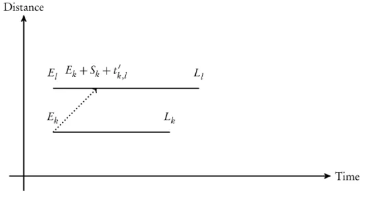
As case 3.2 is the opposite of case 3.1, the next case 3.4 is the opposite of case 3.3. In case 3.4 we have that the latest arrival time of the second macro node requestL_l to occur later then the latest departure of the first macro node requestL_k+S_k plus travel timet_k′_,_l. Formally we can write it as :

L_l ≥L_k+S_k+t_k′_,_l

This condition is illustrated in Figure3.11

Time Distance

E_k L_k

E_l Lk+Sk+t_k′_,_l L_l

Figure 3.11: Latest arrival of the second macro node request is after the latest departure of the first

(41)

of the combined macro node request. Therefore we can set the latest arrival time of the combined macro node request as the latest arrival of the first macro node request.

L_k′=L_k

Similar to the single formulation to handle cases 3.1 and 3.2, we introduce a single formulation to handle cases 3.3 and 3.4

L_k′=mi n(L_k, L_l −(S_k+t_k′_,_l))

3.7.5 Combined macro node request properties

To summarize the full analysis that we performed for all three cases. The resulting properties of the combined macro node request can be computed as follows.

Case one is the only unfeasible case. Therefore the condition to decide if two macro nodescan be combinedis the negation of the condition in case one. Therefore two macro nodes can be feasibly combined, if they obey the following condition:

L_l ≥E_k+S_k+t_k′_,_l

If the two macro nodes obey the stated feasibility condition, then the properties of the resulting macro node request can be computed as

E_k′=mi n(L_k, max(E_k, E_l−(S_k+t_k′_,_l)))

L_k′=mi n(L_k, L_l−(S_k+t_k′_,_l))

S_k′=S_k+S_l+t_k′_,_l+w+

wherew+=max(0,E_l−(L_k+S_k+t_k′_,_l))

Q_k′=Q_k+Q_l

p_{f i r s t}

k′= pf i r s tk p_{l as t}

k′= pl as tl

3.7.6 Vehicle fleet constraints

Until now we have ignored that the VRPTW problem description also defines constraints on the available vehicle fleet, and our macro nodes must respect the constraints imposed by the vehicle fleet. Since we are assuming a homogeneous vehicle fleet, the fleet can be described by:

(42)

3. Macro Nodes 3.8. Summary

• Vehicle working time interval[E_v,L_v]

To respect the capacity constraint we simply check that we never combine two macro nodes whose combined demand quantity exceeds the vehicle capacity.

Q_k+Q_l <Q_max

To respect the time window constraint we have to check two things.

1. That the latest arrival time at a macro node request is not narrowed beyond the time a vehicle can’t arrive to it.

2. That the latest departure time from a macro node request is not later then the working time window of a vehicle.

Hence, when combining two macro node requestsr_m

k =〈Ek,Lk,Sk,Qk,pf i r s tk,pl as tk〉andrml =

〈E_l,L_l,S_l,Q_l,p_{f i r s t}

l,pl as tl〉into macro node requestrmk′ =〈Ek′,Lk′,Sk′,Qk′,pf i r s tk′,pl as tk′〉. This

macro node request must satisfy the following two conditions.

E_v+t_{d e pot}_,_p

f i r s t_k_′ ≤Lk′

and

L_k′+S_k′+t_p

l as t_k_′,d e pot≤Lv

The first condition ensures that if a vehicles departs from the depot as early as it can (i.e. at time E_v) and travels the distance until the macro node in timet_{d e pot}_,_p

f i r s t_k_′ it will still be able to service

the macro node, because it arrives before the latest arrival timeL_k′.

The second condition ensures that departing at the latest feasible timeL_k′+S_k′and taking the

traveling time needed to go back to the depot. A vehicle still arrives back to the depot before its finishing timeL_v.

3.8 Summary

(43)

4

Cluster Construction

The previous chapter introduced the theoretical foundations for combining requests into macro nodes and encoding these macro nodes as individual requests. This chapter discuses the practical aspects of implementing the before-mentioned clustering algorithm. Also, it will introduce and provide motivation for several heuristic metrics which allow to compare the adequacy of combining two macro nodes together.

4.1 Clustering Algorithm

Our approach for macro node construction is based on the idea that one macro node is appended to the end of another macro node. This approach is similar to the way insertion heuristics construct routes. We adopted the idea used by insertion heuristics but instead of building routes we modify it to construct macro nodes.

Analysis from the previous chapter allows to decide when two macro nodes can be feasibly combined. This guarantees that any macro node that we construct is always serviceable by a vehicle.

4.1.1 Pseudo Algorithm