NETWORK FLOW ORIENTED APPROACHES FOR VEHICLE SHARING RELOCATION PROBLEMS

doi: 10.1590/0101-7438.2017.037.03.0455

NETWORK FLOW ORIENTED APPROACHES FOR VEHICLE SHARING RELOCATION PROBLEMS

Alain Quilliot

_{, Samuel Deleplanque}

_,

Antoine Sarbinowski

and Annegret Wagler

Received April 24, 2017 / Accepted November 30, 2017

ABSTRACT.Managing a one-way vehicle sharing system means periodically moving free access vehicles from excess to deficit stations in order to avoid local shortages. We propose and study here several net-work flow oriented models and algorithms which deal with a static version of this problem while unifying

preemptionandnon preemptionas well ascarrier riding cost,vehicle riding timeandcarriernumber min-imization. Those network flow models are vehicle driven, which means that they focus on the way vehicles are exchanged between excess and deficit stations. We perform a lower bound and approximation analysis which leads us to the design and test of several heuristics. One of them involves implicit dynamic network handling.

Keywords: Network Flow, routing, Vehicle sharing.

1 INTRODUCTION

Vehicle Sharingsystems [14, 20, 28, 29] are emerging mobility systems which aim at compro-mising between purely individual mobility and rather rigid public transportation. Such a system is composed of a set ofstations, at which free accessvehiclesare parked. Thosevehiclesmay be bicycles or electric cars. There exists a special station calledDepot, in which a set ofcarriers (trucks, self-platoon convoys, . . . ) are waiting: they periodically exchangevehiclesbetween the stations and eventually provide them with additionalvehicles. A trend is to make the system be aone-waysystem: users are not imposed to givevehiclesback at thestationswhere they picked them up. This feature makes the system more attractive, but also raises the eventuality of unbal-anced situations: stations may become overfilled other under-filled, provoking local shortages or making users unable to give theirvehiclesback. This makes arise two decision problems:

*Corresponding author.

1LIMOS CNRS 6158, Labex IMOBS3, UCA Clermont-Ferrand, France. E-mail: alain.quilliot@isima.fr 2ULB, Bruxelles, Belgium. E-mail: deleplanque.samuel@gmail.com

– a strategiclevel problem [8, 9, 14, 25, 29], about the way stations are located and ca-pacitated and about the pricing of the system [29]. One must simultaneously maximize some globalAccess Demand, and minimize costs which involve not only infrastructure costs but also running costs related to periodicalvehiclerelocation. Though thisVehicle Sharing Station Location(VSSL) problem looks like a standardFacility Location prob-lem [13, 19, 22, 26, 30], addressing it is difficult in practice, since estimating the way Access Demanddepends on the way stations are located can only be done through rough approximation.

– anoperational (or tactical) level problem (see [5, 6, 7, 10, 11, 18, 20, 21, 23, 24, 25, 27]), about the wayvehiclesare periodically moved fromexcesstodeficitstations in order rebalance the system (Relocation Process). Performing this process while meeting both economic and quality of service purposes means addressing aVehicle Sharing Relocation problem (VSR).

This contribution is devoted to the operational level, that means to the VSR Problem, which also appears as a slave sub-problem in any bi-level VSSL formulation. Related VSR models may be:

– static: at some time during the process,excessanddeficitstations are identified, together withexcessanddeficitamount ofvehicles. One must make thecarriersmovevehiclesfrom excesstodeficitstations, while minimizing some operational cost, function of thevehicle riding time, of the number ofcarriers and of thecarrier riding time, while keeping the total duration of the process from exceeding amakespanthreshold;

– dynamic: one knows, for every stationx, at which timevehiclesare going to be demanded or given back by the users. Then one schedules thecarriersin order to meet most demands and avoid any unbalanced situation, while minimizing some operational cost;

– on line: the context is the same as in the dynamic case, but knowledge about demands is incomplete and uncertain.

Preemption may be allowed: a carrier may load somevehicle at some station and drop it at another station, before some other (or eventually the same) carriercomes, loads it again and brings it until a third station.

Some authors consider time indexed requests [11, 27] and address the resulting model through a Benders decomposition scheme. None of them linksnon preemptionandpreemption, while, even if not practical from the point of view of a central manager,preemptionmay be used as a relaxation ofnon preemptionand help into designing algorithms.

More, one may notice that a common feature of the above mentioned static and dynamic models is that they arecarrieroriented [24, 25], in the sense that they focus on the construction of the recollection tours which are run by thecarriers, and consider the routing of thevehiclesinside thecarriersas a kind of slave object [10]. Such an approach may be criticized because of the lack of a backward link between the mastercarriertour collection and thevehiclesub-problem: the search for the mastercarriertour collection is then performed in a somewhat blind way (genetic algorithms, . . . ).

So we adopt here the opposite point of view and consider that performing arelocationprocess means routingvehiclesfromexcess stationstodeficitones in a way which make them share, as often as possible, related carriers. This leads us to propose models which stress the role played by thevehiclenetwork flow induced by the relocation process, and then derive alternative approaches tocarrier drivenones, which we say to bevehicle driven: thevehiclerouting strategy becomes the master object, which determines in turn thecarrier routes. This allows us to link preemptiveandnon preemptiveVSR models and point out that understandingpreemptionas a relaxation ofnon preemptionleads us to a commonNetwork Flowframework.

The paper is organized as follows. We first provide (Section 2) a general framework for both preemptiveandnon preemptivestatic VSR, which mixes several performance criteria: economic cost of therelocationprocess (carrier numberandcarrier riding cost), and quality of service (unavailability of thevehiclesduring the process). We reformulate resulting models asNetwork Flowmodels, making appearpreemptionas a relaxation ofnon preemption. We keep on (Sec-tion 3) by performing a lower bound analysis of this VSR model. In Sec(Sec-tion 4, we propose a first heuristic scheme, which considers the wayvehiclesare distributed fromexcess stationsto deficitones as the master object of aMin Cost Assignment/Pick up and Deliveryhierarchical de-composition scheme, and state an approximation result for what we call themin-cost assignment strategy. In Section 5 and 6, we propose and test heuristics, which deal with aggregatedvehicle andcarrierflow vectors and turn them into solutions of respectivelyNon Preemptiveand Pre-emptiveVSR. One of those heuristics involves the implicit management of large size dynamic network.

2 VSR PREEMPTIVE AND NON PREEMPTIVE CARRIER ORIENTED MODELS

VSR (Vehicle Sharing Relocation Problem) Instances: We consider here a set X ofstations, one of them being a specificstation Depot. Any stationx is provided with a coefficientv(x), which tells us that v(x) vehicles are in excess at station x: if v(x)is strictly negative, then carriersneed to bring –v(x)vehiclesto stationx(xis then said to be adeficitstation); ifv(x)

ifv(x)=0 thenxis said to beneutral.Carriersare initially located atDepotand they all have a same capacityCAP. We suppose thatx∈Xv(x)=0, which means that some stations may be used to bring additionalvehiclesto the system, or, conversely, to remove some of them. We also suppose thatDepotisneutral. Any stationxis provided with a capacityC(x).DISTdenotes the X.X timematrix: DISTx,y is the time required for acarrier to go from stationx to station y. T-Maxis the maximalmakespanof therelocationprocess: the total time for this process cannot exceed T-Max. By the same way,COST denotes theX.X carrier cost matrix:COSTx,y is the integrated cost (energy, human resource, . . . ) induced by a move of acarrier from stationxto station y, when this move is performed inDISTx,y time units. Both matricesDISTandCOST satisfy theTriangle Inequalityand are such thatCOSTx,x =DISTx,x =0 for any stationx. Idle-Costdenotes thewaiting costinduced for acarrierwhen it remains at any stationx =Depot during one time unit. We suppose (Extended Cost Hypothesis) that if acarriermoves fromxto yat a reduced speed in timet ≥DISTx,y, then the induced extended costE-COSTx,y,t is equal toCOSTx,y+Idle-Cost.(t−DISTx,y). All this defines aVSRinstance (X,v,C,CAP,T-Max, DIST, COST).

2.1 Non Preemptive VSR Model

AVSR tourŴis a finite sequenceŴRout e = {x0 =Depot,x1, . . . ,xn(Ŵ) = Depot}of stations,

which is called aroute, given together with a loading strategy, that means with 2 sequences

ŴLoad = {L0 = 0,L1, . . . ,Ln(Ŵ)}andŴTime = {T0 ≥ 0,T1, . . . ,Tn(Ŵ)}of coefficients whose

meaning is: acarrierwhich follows the routeŴRouteloads, at timeTi,Li vehicles at stationxi (unloads in case Li <0). The length ofŴRoutein theCOSTsense is given byL-COST(ŴRoute) = jCOSTx j,xj+1. The length ofŴRoutein theDIST sense is given byL-DIST(ŴRoute)= j DISTx j,x j+1. The costL-E-COST(Ŵ) ofŴis given by:L-E-COST(Ŵ)=L-COST(ŴRoute)+ Idle-Cost.(Tn(Ŵ) −T0). For any i, we denote by L∗i = j=0..iL j the load of thecarrier when it leaves stationxi.

ThisVSR tourŴisNon PreemptiveVSRfeasibleif:

• For anyi =0, . . . ,n(Ŵ)−1,T-Max≥Ti+1≥Ti+DISTxi,xi+1; (E1)

• For anyi =0, . . . ,n(Ŵ)−1, 0≤L_i∗=j=0...iL j≤CAP; (E2)

• j=0...n(Ŵ)Lj =0; (E3)

• For any jsuch thatv(xj)≥0(v(xj)≤0), then

v(xj)≥L j ≥0(v(xj)≤L j≤0). (E4)

Explanation: (E1): Acarrierneeds at leastDISTxi,xi+1time units to go fromxi toxi+1; (E2,

Given scaling coefficientsα, β, δ together with a VSR instance (X,v,C,CAP, T-Max,DIST, COST), we set:

Non Preemptive VSR Model: {Compute a VSR feasible tour collection Ŵ∗ = (Ŵ(k), k=1. . .K)such that:

• For any station x:ki such that x(k)i=xL(k)i =v(x). (E5)

• Minimize Global-Cost(Ŵ∗)=α.K+β.kL-E-COST(Ŵ(k))+ δ.(kj(DISTx(k)j,x(k)j+1.L∗(k)j)}.

Explanation: (E5): For anyexcess station x, v(x)vehicleshave to be picked up inx, and for any deficit station x,−v(x)vehicleshave to be delivered tox. Global-Cost(Ŵ∗)is a weighted sum of thecarrier number, thecarrier riding cost, and thevehicle riding time(timevehiclesspend into thecarriers).

Remark 1. Because of non preemption, every move fromx(k)i to x(k)i+1 inŴ(k) may be

performed in exactlyDISTx(k)i x(k)i+1 time units; Thusk L-E-COST(Ŵ(k)) may be replaced bykL-COST(Ŵ(k)Route. By the same way, anyneutralstations but theDepotstation may be removed from the input of theNon PreemptiveVSR model.

Remark 2 (About MIP Models and Complexity).ModelingVSRthrough a MIP (Mixed Integer Linear Program) is possible, but inefficient. The reason is that there is no a priori bound about the number of times a given station is going to be visited by a samecarrier. As for complexity, in the case whenK =1 (αvery large),v(x)values are equal to 1 or−1,CAP=1 andδ =0, our problem is equivalent to theTravelling SalesmanProblem set on a bipartite graph (theexcess stationson one side and thedeficitones on the other side), which is NP-Hard. Non Preemptive VSRalso contains theUncapacitated Swapping Problem, which is also NP-Hard (see [1]).

2.2 Loading Strategy Flow Model Related to a VSR Route CollectionŴ∗_Route

Let us suppose now that we are provided with a collectionŴ_Route∗ = {ŴRout e(1), . . . , ŴRoute(K)} ofK carrier routes, all with length≤T-Max. Following [10], we define a networkH(ŴRoute)as follows (see Fig. 1):

• Nodes ofH(Ŵ_Route∗ )are:

◦ copies of the nodesx(k)j ofŴRoute(1), . . . , ŴRoute(K)considered as being all dis-tinct;

◦ a sourcesand a sinkp;

◦ nodesExc(x),x ∈X,excessnodes;

• ArcseofH(ŴRoute)and related costsCeare:

◦ Route arcs e = (x(k)j,x(k)j+1) of the routes ŴRoute(k), with cost Ce = DISTx(k)j,x(k)j+1;

◦ Excess arcs e=(Exc(x),x(k)j),x∈ X,x excess, such that the image inXofx(k)j isx, withCe=0;

◦ Deficit arcs e=(y(k)j,Def(y)),y deficit, such thaty(k)j isy, withCe =0;

◦ Input arcs e=(s,Exc(x)),x excess, andoutput arcs e=(Def(y),p),y deficit, with Ce=0.

Figure 1

Then we may set:

Load-NP-VSR Model:{Compute on H(Ŵ∗_{Rout e})a non negative integral arc indexed flow vector Z such that:

◦ for any route arc e,Ze≤C AP;

◦ for any input arc e=(s,E xc(x)),xexcess,Ze=v(x);

◦ for any output arc e=(De f(y),p),yde f icit,Ze= −v(x);

◦ Cost C.Z=eCe.Zeis the smallest possible}.

This construction yields, as in [10]:

Proof. Any loading strategy related to the tour collection Ŵ∗ may be turned into a feasi-ble solution ofLoad-VSRwhose cost is exactly thevehicle riding time: k, j (DIST(x(k)j, x(k)j+1).L∗_j). Conversely, any flow vector Z which is a feasible solution ofLoad-NP-VSRcan

be interpreted as aloading strategy.

It comes thatNon PreemptiveVSR may be reformulated:

Non Preemptive VSR Reformulation: {ComputeŴ∗_{Rout e} = {ŴRout e(1) . . . , ŴRout e(K)}, to-gether with an optimal Load-NP-VSR solution Z(Ŵ∗_{Rout e}), which minimize:

α.K +δ.C.Z(Ŵ∗_{Rout e})+β.kL−C O ST(Ŵk)}.

2.3 Preemptive VSR Model

In case preemption is allowed, then we say that theVSR tourŴis preemptive VSR feasibleif (E1, E2, E3) are true. Besides, for any collectionŴ∗ = (Ŵ(k),k = 1..K ≤ K-Max)of such non-preemptive feasible tours, we set, for any time valuet, and any stationx:

– (Ŵ,x,t)= {(k,j),k=1. . .K,j=0. . .n(Ŵ(k)), such thatx(k)j =xandT(k)j ≤t};

– H(Ŵ,x,t)=Sup(0, v(x))−(k,j)∈(Ŵ,x,t)L(k)j.

Clearly,H(Ŵ,x,t)denotes the number ofvehicleswhich are really located in stationx at time t after all loading/unloading transactions have been performed. Then we say that the collection

Ŵ=(Ŵ(k),k =1. . .K ≤ K−Max)is afeasiblesolution for thepreemptive VSRinstance (X, v,C,CAP,T-Max,DIST, COST) if everyŴ(k)ispreemptive feasible, if (E5) holds and if, for any time valuetand any stationx: 0≤ H(Ŵ,x,t)≤C(x). (E6)

(E6) expresses the fact that, at any timet, the number ofvehiclescurrently located atxis non negative and cannot exceed the capacity of the stationx. Then we may set:

Preemptive VSR Model:{Compute a preemptive VSR feasible tour collectionŴ∗=(Ŵ(k),k=

1. . .K)such that (E1, E2, E3, E5 and E6 hold) and which minimizes the following global cost:

• Global-Cost(Ŵ∗)=α.K+β.kL-E-COST(Ŵ(k)) +δ.(kj(DISTx(k)j,x(k)j+1.L∗(k)j))}.

T and leaves it at timeT+t,vehiclesunloaded at timetand loaded again at timeT+t(provided C(x)is large enough) are not involves in thisvehicle riding timesince they are available for users betweenT andT +t.

Remark 4.Taken together, aboveNon PreemptiveandPreemptiveVSR models extend [5, 7, 10, 11, 14, 25], since they unifypreemptionandnon preemption, and mixcarrier numbers, vehicle riding timeandcarrier riding costinto a same criterion. Still, in case of non feasibility, we do not take into account, as in [10, 11], the eventual deviation between the wanted balanced state and the true state of the system at the end of the process.

2.4 A Network Flow Framework

Let us recall that aflow vectordefined on a networkG=(N,A), with node set Nand arc setA, is a rational (or integral) valuedA-indexed vectorgsuch that, for any nodez, the followingflow conservation lawholds:

esuch thatorigin(e)=zge=esuch thatdestination(e)=zge

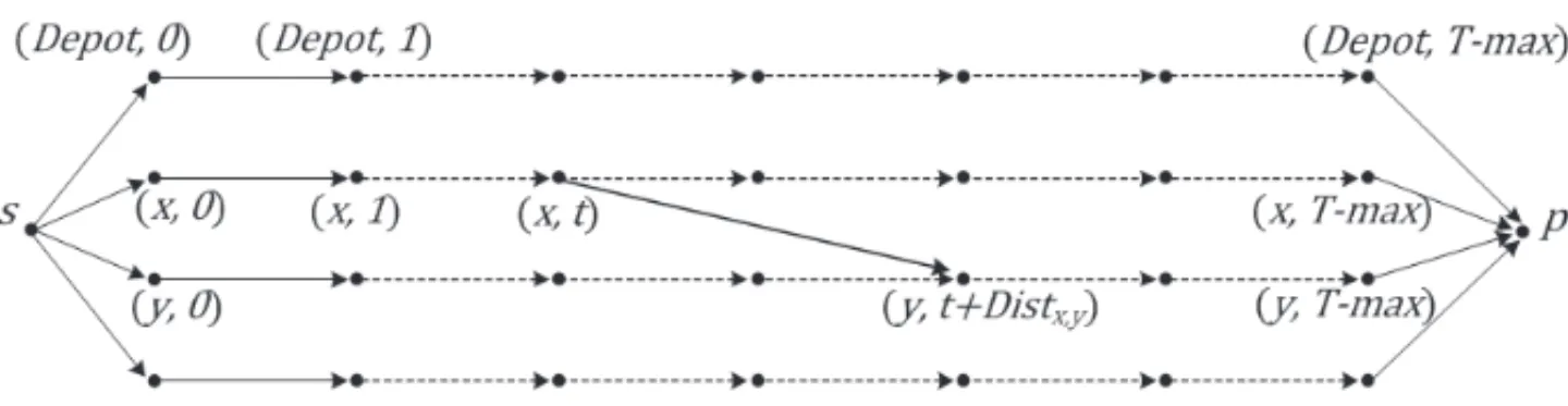
Let us now suppose that all values DISTx,y are integral (it is always possible to do it). Then we derive from the VSR instance (X,v,C,CAP,T-Max,DIST, COST) adynamic network[4] GT-Max=(XT-Max,ET-Max)as follows (see Fig. 2):

– XT-Maxis the set of all pairs (x,t),x ∈ X,t = 0. . .T-Max, augmented with 2 nodess (source) andp(sink);

– ET-Maxincludes:

◦ Inputarcs(s, (x,0))and((x,T-Max),p), with nullvehicleandcarriercosts;

◦ idlearcs((x,t), (x,t+1))Out, with nullvehicleandcarriercosts;

◦ carrier-idlearcs((x,t), (x,t +1))Inwith unitvehiclecosts andcarriercosts equal toβ.Idle-Costifx=Depotand 0 else;

◦ activearcs((x,t), (y,t+DISTx,y), withvehiclecosts equal toδ.DISTx,yandcarrier cost equal toβ.COSTx,y;

◦ backwardarc(p,s)with nullvehiclecosts andcarriercosts equal toα.

Then, we may set on this network the following multi-commodity flow model:

Network-Flow-VSR Model:{Compute non negative integral flow vectors F and f , respectively carrier and vehicle flow vectors, such that:

◦ For any idle arc e=((x,t), (x,t +1))Out, fe ≤C(x)and Fe=0; (E7)

Figure 2–Dynamic NetworkGT-Max=(XT-Max,ET-Max).

◦ For any active arc e=((x,t), (y,t+DISTx,y), fe≤C AP.Fe; (E9)

◦ For any x =Depot,F(s,(x,0))=F((x,T-Max),p)=0; (E10)

◦ For any node x =Depot, f(s,(x,0))=Sup(v(x),0)and

f((x,T-Max),p)=Sup(−v(x),0); (E11)

◦ F and f minimize CostT-Max(F, f)=e∈ET-MaxFe.Carrier-Coste

+e∈ET-Maxfe.Vehicle-Coste.}

Explanation:Flow Conservation lawexpresses the circulation ofcarriersandvehiclesbetween the stations. Carrier-idleandidlearcs make the difference betweenvehicleswhich are waiting at some stationxwhile being located either inside somecarrieror outside. (E9) says that any vehiclemoving between 2 stationsx,ymust be contained into somecarrier. (E10, E11) provide us with initial and final states of bothcarriersandvehicles.

Theorem 1.Solving Network-Flow-VSR is equivalent to solving Preemptive VSR.

Proof. We first notice that, if afeasible preemptive VSR tour collection Ŵ∗ = (Ŵ(k),k =

1..K ≤K-Max)is given, then theExtended Cost Hypothesisimplies that inequalities (E1) may be supposed to be tight in casexi =xi+1. It comes thatŴmay be turned into a feasible

Network-Flow-VSRsolutionF,f, with same cost, by setting:

– F(p,s)=K;

– For anycarrier-idlearce=((x,t), (x,t+1))In:

◦ Fe =number ofcarriers k located inx betweent andt +1 according to the tours

Ŵ(k);

◦ fe =the sum of all quantitiesL∗(k)j, taken for allcarriers kas above and j such thatx(k)j =x,x(k)j+1 =x,T(k)j ≤t,T(k)j+1>t;

– For anyidlearce=((x,t), (x,t+1))Out:Fe=0 and fe =H(Ŵ,x,t);

◦ Fe=number ofcarriers ksuch thatŴ(k)involves a move fromxtoyat timet;

◦ fe = sum of all L∗(k)j, for all k as above and j such that x(k)j = x, x(k)j+1=y,T(k)j =t;

– For any arce = (s, (x,0))(e =(Depot,T-Max),p),Fe and fe are defined according to (E10) and (E11).

Conversely, if(F, f)is someNetwork-Flow-VSRfeasible solution, then we know that F may be decomposed as a sum of {0,1}-valued flow vectors F(k),k = 1. . .K = F(p,s). Those

elementary flow vectors F(k),k = 1. . .K, define in a canonical way routesŴ(k)Route, to-gether with date sequencesŴ(k)Time. Then, for any arce = ((x,t), (y,t +DISTx,y)ande = ((x,t), (x,t+1))In, we decompose feas a sum of non negative values fe(k), with values no more thanCAP. This allows us to deduceloading sequencesŴ(k)Load= {L(k)0,L1, . . . ,L(k)n(Ŵk))},

k=1. . .K, according to a basic j =0, . . . ,n(Ŵ(k)indexed iterative process. We easily check that the resultingtourcollectionŴ(k),k=1. . .Kispreemptive VSRfeasible, with a global cost

Global-Cost(Ŵ∗)exactly equal toCostT-Max(F, f).

Let us now try to extend Lemma 0 to this framework. In order to do it, we consider acarrier flow vector F and denote by X(F)the node subset of XT-Maxwhich contains s,p, all nodes (x,0)and(x,T-Max), together with all nodes(x,t)which are origin or extremity of some arc e=((x,t), (y,t+DISTx,y),x = y, such thatFe=0. We provideX(F)with an arc setE(F) which contains arcs(s, (x,0)), (x,T-Max),p),x∈ X, as well as:

– relatedactivearcse=((x,t), (y,t+DISTx,y),x =y;

– extended idlearcs ((x,t), (x,t′))In and((x,t), (x,t′))Out, witht,t′such that no(x,t′′)

exists in X(F)such that t < t′ < t′′; those arcs are provided withvehicle-cost values respectively equal to(t′−t)and 0;

Since valuesFedefined onidlearcse=((x,t), (x,t+1))Incan be turned in a natural way into valuesFedefined onextended idlearcs((x,t), (x,t′))In,F may be viewed as a flow vector on the network(X(F),E(F)). Then we set:

Load-P-VSR:{Compute, on the network(X(F), E(F))a non negative flow vector f , such that:

• For any active arc e=((x,t), (y,t+DIST(x,y),x=y and any extended-idle arc

e=((x,t), (x,t′))In we have fe≤CAP.Fe;

• For any station x, f(s,(x,0))=Sup(v(x),0)and f((x,T-Max),p)=Sup(−v(x),0);

This allows us to state the following extension of Lemma 0 (proof left to the reader):

Lemma 1. F being given, solving Load-P-VSR provides us with an optimal loading strategy. One may now ask about castingNon Preemptive VSRinto thisNetwork Flowframework. This leads us to set:

NP-Network-Flow-VSR Model: {Compute K and two non negative integral multi-commodity flow integral vectors F = (F(k),k = 1. . .K)and f = (f(k),k = 1. . .K), respectively carrier and vehicle multi-commodity flow vectors, such that:

◦ For any k,F(k)is{0,1}-valued; (E12)

◦ For any idle arc e=((x,t), (x,t+1))In,

x=Depot,kf(k)e =kF(k)e =0; (E13)

◦ For any idle arc e=((x,t), (x,t+1))Out,

x=Depot,kF(k)e =0; (E13-1)

◦ For any idle arc e=((Depot,t), (Depot,t+1))Out,kf(k)e =0; (E13-2)

◦ For any active arc e=((x,t), (y,t+DISTx,y), f(k)e ≤CAP.F(k)e; (E14)

◦ For any x =Depot,kF(k)(s,(x,0))=kF(k)((x,T-Max),p)=0; (E15)

◦ For any x =Depot,kf(k)(s,(x,0)) =Sup(v(x),0)and

kf(k)((x,T-Max),p)=Sup(−v(x),0); (E16)

◦ For any k and any excess (deficit, neutral) station x, values

f(k)e,e=((x,t), (x,t+1)In,

are decreasing (increasing, stationary) when t increases; (E17)

◦ F and f minimizee∈ET-MaxFe∗.Carrier-Coste+e∈ET-Maxfe∗.Vehicle-Coste.}

Theorem 2.Solving NP-Network-Flow-VSR is equivalent to solving Non Preemptive VSR.

Proof. It is pure routine to check that anyNon PreemptiveVSR feasible solutionŴ∗gives rise to a feasible solution(F, f)ofNP-Network-Flow-VSRwith the same cost value. Conversely, monotony constraint (E17) forbids anycarrier k from unloading (loading) at someexcess or neutral(deficitorneutral) stationx, enabling us to turn flow vector f(k)into aloading strategy for the tourŴ(k)induced by{0,1}-valued flow vectorF(k).

3 VSR LOWER BOUNDS

We propose here 2 classes of easy to computevehicle drivenlower bounds for theVSRProblem: the first one relies on Min-Cost Assignmentmodels which separately bound theactive carrier number, thecarrier riding costand thevehicle riding time. The second one directly derives from the previousNetwork-Flow-VSRmodel.

3.1 Min-Cost Assignment Based Lower Bounds Let us consider the following ILP models:

VMCA Vehicle-Min-Cost-Assign:{Compute integral vector Q =(Qx,y, x excess, y deficit)≥ 0, such that:

◦ For any excess station x,y deficit stationQx,y =v(x)

◦ For any deficit station y,x excess stationQx,y = −v(y)

◦ Minimizex,yDISTx,y.Qx,y}

LB-VMCAdenotes the related optimal value, which may be computed while relaxing the inte-grality constraint on the vectorQ. In any case (preemptionor not),LB-VMCAprovides us with a lower bound of thevehicle riding time:Ŵkj (DISTx(k)j,x(k)j+1.L∗_j).

CMCA Carrier-Min-Cost-Assign: {Compute integral vector R = (Rx,y,x,y stations) ≥ 0, such that:

◦ For any neutral station x=Depot,y Rx,y =0=yRy,x

◦ For any excess station x, CAP.y Rx,y =CAP.y Ry,x ≥v(x)

◦ For any deficit station y, CAP.x Rx,y =CAP.x Ry,x ≥ −v(y)

◦ y RDepot,y =y Ry,Depot≥1

◦ Minimizex,yCOSTx,y.Rx,y}

LB-CMCA denotes the related optimal value, which may be computed in polynomial time through a simpleMin Cost Flow algorithm.LB-CMCA is a lower bound for thecarrier rid-ing costkL-E-COST(Ŵ(k)). IfLB-Time-CMCAis the value of theCMCAmodel obtained by replacing theCOST matrix by theDISTmatrix, thenLB-Time-CMCA/T-Maxis a lower bound for thecarrier number K.

◦ For any neutral station x =Depot, yRx,y =0=yRy,x

◦ For any x,y, both deficit or both excess, Rx,y =0

◦ For any y deficit, RDepot,y=0and for any x excess, Rx,Depot =0

◦ For any excess station x, y deficit or Depot Ry,x =y deficitRx,y =v(x)

◦ For any deficit station y,x excess or DepotRy,x =x excessRx,y = −v(y)

◦ y excessRDepot,y =yRy deficit,Depot=1

◦ For any subset A⊆X− {Depot},A=Nil, x∈Ay,y∈/ARx,y ≥1(No-Subtour Constraint)

◦ Minimizex,yCOSTx,y.Rx,y}

LB-UCMCAdenotes the related optimal value. We see thatLB-UCCAis a lower bound for the L-COSTvalue of any tourγ which starts and ends intoDepot, while alternatively moving from excessnodes todeficitnodes and carrying unit loads. IfLB-Time-UCMCAis the optimal value of theUCMCAmodel obtained by replacing theCOSTmatrix by theDISTmatrix, then LB-Time-UCMCAis a lower bound for thecarrier riding time L-DIST induced byγ. UCMCAinvolves significantly less variables than theCMCAmodel.

We deduce:

Theorem 3. A VSR (Preemptive or Not) lower bound is given by LB-MCA = α LB-Time-CMCA/T-Max+β.LB-CMCA+δ.LB-VMCA.

Proof. It is contained into the comments which come together with the definition of the above

models.

Theorem 4.A Non Preemptive VSR lower bound is given by LB-UMCA=αLB-Time-UCMCA/ (CAP.T-Max)+β.LB-UCMCA/CAP+δ.LB-VMCA.

Proof. Anytourγ which satisfies (E1, E2, E3, E4) may be split intoCAP toursγ1, . . . , γCAP, all with same lengths, which globally perform therelocationprocess when relatedCAP = 1. It comes from the fact that any solution Z of theLOAD-NP-VSRmodel related to γ may be decomposed into a sumZ1+ · · · +ZCAPof{0,1}-valued flow vectors. So, ifCarrier-Ride-Time1

andCarrier-Ride-Cost1respectively denote the smallest possible values for thecarrier riding

timeand thecarrier riding costrelated to the case whenCAP= 1 andT-Max= +∞, we see that: thecarrier riding time (carrier riding cost)of any solutionŴofNon Preemptive VSRis at least equal toCarrier-Ride-Time1/CAP (Carrier-Ride-Cost1/CAP). We deduce thatα.⌈

Carrier-Ride-Time1/CAP.T-Max⌉ +β Carrier-Ride-Cost1/CAP +δ.LB-VMCAis aNon Preemptive VSR

lower bound. ButCarrier-Ride-Time1corresponds to a kind of TSPcarrier tour starting and

3.2 Projected Flow Lower Bound

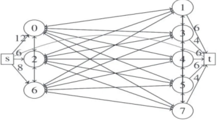
We derive from the dynamic network GT-Max = (XT-Max,ET-Max)of Section 2.4 aprojected networkGProj=(XProj,EProj)as follows (see Fig. 3):

◦ XProj=X∪ {s,p}where nodessand pare additional nodessourceandsink;

◦ The restriction ofGProjtoX is a complete network: any arce=(x,y)is provided with acarrier costCCe = β.COSTx,y+(α/T-Max).DISTx,y and with avehiclecostCVe = δ.DISTx,y.

◦ There is an arc(s,x)fromsto anyexcess station x, with nullcarrierandvehiclecosts;

◦ There is an arc(y,p)from anydeficit station ytop, with nullcarrierandvehiclecosts;

◦ There is abackwardarc(p,s), with nullcarrierandvehiclecosts.

Figure 3–A networkGProjderived from 3 excess stations and 5 deficit stations.

Then we set:

Projected-VSR-Flow Model:{Compute on the network GProjtwo integral flow vectors H and h such that:

◦ For any arc e=((x,y),x,y=s,p,he≤CAP.He (E18)

◦ For any excess (or neutral) station x,h(s,x) =v(x)and

for any deficit station y,h(y p)= −v(x) (E19)

◦ yHDepot,y =yHy,Depot≥1 (E20)

◦ MinimizeeCCe.He+eCVe.he.}

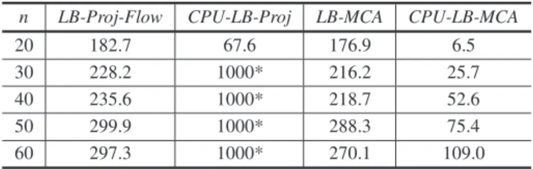
We denote byLB-Proj-Flowthe related optimal value of this program. Then we state:

Proof. Any feasible solution F, f ofNetwork-Flow-VSR can be turned into a feasible solu-tionH,h ofProjected-VSR-Flow. The costCostT-Max(F, f) = e∈ET-MaxFe.Carrier-Coste+

e∈ET-Max fe.Vehicle-Costemay be decomposed into:

CostT-Max(F, f)=α.F(p,s)+e∈ET-Max,e=(p,s)Fe.Carrier-Coste+e∈ET-Max fe.Vehicle-Coste.

Through projection, the two last terms of this sum give rise to the quantityarcs eβ.COSTe.He+ arcs eCVe.he. The first component corresponds toα.K, whereK =F(p,s)is thecarrier number.

But we know that thiscarrier numberis at least equal to(e=(x,y)∈E-Proj Hx,y.DISTx,y)/T-Max. We deduce the first part of our statement.

As for the second part, we get it by noticing that any solutionH,h of theProjected-VSR-Flow program give rise in a natural way to a feasible solutionRof theCMCAprogram and a feasible solution Q of theVMCA program, and by keeping on with the above decomposition of the quantityarcs eCCe.He+arcs eCVe.he.

Remark 6. TheProjected-VSR-Flowmodel does not solve ourVSRproblem, even according to itspreemptiveversion. For instance one may consider astationset X = {Depot,A,B,C}, acarrier flow H related to theroute (Depot,A,B,C,A,Depot)followed by 1 carrier with capacity 1, and avehicleflowhwhich routes 1 flow unit fromexcess station Ctodeficit station B. Then thecarriercannot deliver its load inBbefore picking it up inC.

Remark 7. LB-Proj-Flowvalue provides us with a better lower bound than theLB-MCAlower bound of Theorem 3. Still,Projected-VSR-Flowis a complex NP-Hard model, whose rational relaxation yields a poor lower bound as soon as CAP is large. TheLagrangeanrelaxation of the coupling constraint (E18) yields aLagrangeanvalue Supλ∈(Infh(CV +λ).h)+InfH(CC− λ).H)where:

◦ Vector flowhis subject to (E19) and vector flowH is subject to (E20);

◦ = {λ such that the restriction of the graphGProj to X does not contain any negative

(CC−λ)-circuit}.

But, because of the total unimodularity of flow constraint matrices, this value is the same as the value obtained by performingLagrangeanrelaxation of (E18) on the rational relaxation of Projected-VSR-Flow. That means that the above Lagrangean value does not improve the standard relaxation of the integrality constraint.

4 A VEHICLE MIN-COST ASSIGNMENT BASED HEURISTIC FOR NON PREEMPTIVE VSR

4.1 MCA/PDP Decomposition

Let us recall that aPick-up&Deliveryinstance (see [2, 12, 17]) is defined by:

◦ a setJofrequests j=(o(j),d(j), λ(j)), whereo(j),d(j)andλ(j)are respectively the origin, thedestinationand theloadof j;Ndenotes the set of all nodeso(j),d(j),j∈ J, augmented with aDepotnode and considered as pairwise distinct; theserequestshave to be served bytrucks, initially located inDepotand all with capacityCH;

◦ 2 distance matricesDandCS, indexed on the setN.N and a thresholdD-Max;

◦ Scaling coefficientsA,B,C.

A collectionρoftruck routesρ(m),m =1. . .M defined on the setN is afeasible PDP solu-tion if:

◦ everyrequest jis serviced by sometruck m:mfirst loadsλ(j)ato(j)and unloads it into d(j);

◦ the load of atrucknever exceeds capacityCH;

◦ theD-lengthof ρ(m)of anytruck routeλ(m),m=1..M, never exceedsD-Max.

It is an optimalPDPsolution if it isfeasibleand minimizes a quantity:

PDP-COST(ρ)=A.M +B.mCS-Length(ρ(m))+C.jλ(j).D-Ride(j),

whereD-Ride(j)is theD-length which is run by loadλ(j)inside atruck. ALoad-Split PDP instance is defined the same way, but every loadsλ(j)may be split into a sumλ(j)=λ(j)1+ · · · +λ(j)Q(j), of several sub-loads, which are separately handled.

ThoughLoad-Split PDPis NP-Hard, it may be in practice efficiently handled through a GRASP-VNS (Greedy Randomized Adaptative Search + Variable Neighborhood Search) process based uponInsert/Removeoperators:

– Insert operator: Insertingrequest j = (o(j),d(j), λ(j))into some truck route ρ(m)

means:

◦ computing 2 insertion nodesxandyinρ(m), and some sub-loadλ≤λ(j);

◦ insertingo(j)(d(j))betweenx(y)and its successor inρ(m);

◦ addingλto the current load ofρ(m)betweenxandy, and updatingλ(j);

– Removeoperator: Deleteo(j)andd(j)fromρ(m)and update the load ofmand theλ(j)

Then related GRASP-VNS scheme comes as follows:

PDP GRASP-VNS Algorithm

Randomized Initialization:

While allrequestshave not been inserted do

Randomly pick up some non insertedrequest j;

Compute (in a heuristic way)truckparameterm, together with insertion parameters x,y∈ ρ(m), andλ≤λ(j)in such a way that related insertion is feasible and such that (bi-criteria choice):

◦ the induced increase ofPDP-COST(ρ)is the smallest possible;

◦ λis the largest possible;

Local Search Loop:

NotStop;

While NotStopdo

Identify a setJ0⊆ Jofpoorly inserted requests;

Remove J0from Jand reinsert it according to the same process as in the

initializa-tion;

Update the current best solutionρ∗=(ρ(m),m =1..M); UpdateStop.

Let us now come back to ourNon Preemptive VSRinstance, and suppose that, for some instance (X,v,C,CAP,T-Max,DIST, COST), we know, for every pair(x,y),x excess, y deficit station, which quantityQx,y has to move fromxtoy. Then, we only need to solve theLoad-Split PDP instance defined by:

◦ Requests j are all 3-uples(o(j)= x,d(j)= y, λ(j)= Qx,y), taken for all pairs x,y such that Qx,y =0;

◦ D-Max=T-Max;D=DIST;CS=COST;CH=CAP;A=α,B=β, C=δ.

One may conjecture that it is possible to impose assignment vectorQto be an optimal solution, for some cost vectorU =(Ux,y,x Excess,y Deficit)≥0, of the followingVMCA(U)(Vehicle Min-Cost Assignment) model:

VMCA(U):{Compute integral vector Q=(Qx,y, x excess, y deficit stations)≥0, such that:

◦ For any excess station x, y deficit stationQx,y = v(x); For any deficit station y, x excess stationQx,y = −v(y);

Though we cannot prove this conjecture, it leads us to the following reformulation of Non Preemptive VSR:

Non Preemptive VSR VMCA Reformulation: {Compute cost vector U = (Ux,y,x Excess, y Deficit)≥0, such that the optimal value of the related Load-Split PDP instance be the smallest possible}.

We may handle this reformulation through the following algorithmic scheme:

VSR-MCA Algorithm(N : Loop Number)

Initializecost vectorU =(Ux,y,x Excess, y Deficit)≥0;

For j=1. . .Ndo (*Local Searchloop*)

Derive aPDP AssignmentvectorQthrough optimal resolution ofVMCA(U);

Solve (in a heuristic way) the relatedLoad-Split PDPinstance;

Updatecost vectorU;

Apply to the resulting route collection Ŵ∗_Route = {ŴRoute(1), . . . , ŴRoute(K)} the Load-NP-VSRmodel, clean the routesŴRoute(k)from its useless stations;

Keep the best result ever obtained.

Two critical points have to be specified inside this algorithmic description:

1) “Initialize cost vectorU” instruction: LB-MCA lower bound of Section 3 suggests us to apply what we call theShortest Distance/Cost Strategy, and set, for any x,y,x Excess, y Deficit, Ux,y = DISTx,y. +λ.(COSTx,y. +COSTy,x)whereλis some non negative coefficient; as a matter of fact, doing this leads us to extend the above VSR-MCA algorithm into a GRASP algorithmic scheme, by performing initialization of the cost vectorU in a random way:

GRASP-VSR-MCA Algorithm(N : Loop Number, R: Replication Number)

Fori =1. . .Rdo

Randomly generateλ≥0;

For anyx,y,x Excess,y Deficit,Ux,y ←DISTx,y.+λ.(COSTx,y.+COSTy,x);

For j =1. . .Ndo. . .(*Local Searchloop ofVSR-MCA*);

Keep the best result ever obtained.

vector Q, arequestsetReq(U)= {r =(x,y,Qx,y)such that Qx,y =0}and aNon Pre-emptive VSRsolutionŴ∗, whose global costGlobal-Cost(Ŵ∗)may be distributed among requests(x,y,Qx,y)in a natural way:

• The carrier cost α+β.L-COST(Ŵ(k)) related to a givencarrier k is shared between the requests which are served by this carrier, proportionally to the value L-COST (Ŵ(k)x,y).Qx,y, whereŴ(k)x,yis the sub-route which is induced by the restrictionŴ(k)x,y ofŴ(k)betweenxandy(in caseQx,y is split into sub-loads, we deal separately with those sub-loads);

• Everyrequest r = (x,y,Qx,y)is assigned its partL-DIST(Ŵ(k)x,y).Qx,y of thevehicle riding time.

It comes that Global-Cost(Ŵ ∗)may be written Global-Cost(Ŵ∗) = r∈Req(U) Partial-Cost

(r, Ŵ∗), wherePartial-Cost(r, Ŵ∗)is the part ofGlobal-Cost(Ŵ∗)which is charged this way to requestr. Then, for every requestr=(x,y,Qx,y =0)we setVx,y =Partial-Cost(r, Ŵ∗)/Qx,y and updateU as follows:

• IfQx,y =0,Ux,y is replaced by(Ux,y+Vx,y)/2 elseUx,y is unmodified;

• WhenU =U0,Uvalues may be very different fromV values. So we compute the mean valueτ of the ratioVx,y/Ux,y,x,ysuch that Qx,y =0, and replace every valueUx0,y by =τ.U_x0_,y.

4.2 An Approximation Result

A natural question comes about the quality of theShortest Cost/Distance strategy. Since, in most cases, theCOST and DIST matrices are strongly correlated, we consider here the case when those matrices are the same, and whenGlobal-Costonly involves thecarrier riding cost. In such a case, we may state:

Theorem 6 (Shortest Cost/Distance Strategy).If COST=DIST, ifα=δ =0(focus on carrier riding cost minimization) and if T-Max= +∞, then the Shortest Cost/Distance strategy induces an approximation ratio of (1+CAP). This is the best possible ratio.

Proof. We first notice that we may, sinceT-Max= +∞, deal with only onecarrier. Let us first prove the first part of the result, that means that there is no approximation ratio better than (1+CAP). In order to do so, we build the followingNon Preemptive VSRinstance:

– K =1;

– DIST=COSTrepresents the shortest path distance induced on the setXby the following arc setE =E1∪E2∪E3∪E4:

◦ E1= {(Depot,o0,1), (dN-1,1,Depot)}, both arcs with length equal to 1/2;

◦ E2= {(on,c,on,c+1), (dn,c+1,dn,c),n=0..N-1,c=1..CAP−1}, all arcs withsmall lengthε;

◦ E3 = {(on,C A P,dn,C AP),n =0..N-1} ∪ {(dn,1,on+1,1),n = 0..N-2}, all arcs with

length 1;

◦ E4 = {{(on,c,dn−1,c)},n =0..N-1,c=1..CAP}addition being performed modulo N, all arcs with length 1-α, whereαis a small number.

One easily checks that an optimal tour for the carrier is thetour {Depot,o0,1, . . . ,o0,CAP, d0,CAP, . . . ,d0,1,o1,1,...,o1,CAP, . . . ,Depot}, with lengthL-DIST=2n+2n.(CAP-1)ε. For ev-eryn = 0, . . . ,N-1, thistourmakes thecarrier load all theexcess vehicleslocated inexcess stationson,c,c=1. . .CAP, and next bring them todeficitstationsdn,c,c=CAP. . .1, before moving to nodeon+1,1. On another side, the vectorQderiving from theShortest Cost/Distance

strategy is provided byE4. One checks that a related optimalPDPmeets every request related to

an arc(on,c,dn−1,c)through a direct move(on,c,dn−1,c)(proof left to the reader: if it were not the case, then one could remove related arcs ofE4). So, as soon as the carrier has been loading in

stationon,c, it moves to stationdn−1,cand delivers its load. A consequence is that at any time dur-ing the process, the current loads of thecarrierdoes not exceeds 1 and that the optimalPDP solu-tion comes as a sequence{Depot,o0,1,dn−1,1,o0,2,dn−1,1,. . . ,dn−1,CAP,o1,1,...d0,1,. . . ,Depot},

with lengthL-DIST=CAP.n(1−α)+n.CAP.(1+(CAP-1).ε+2n+n.(CAP-1)ε. We conclude.

In order to prove the first part of the result, that means that (1 +CAP)provides us with an approximation ratio, we first notice that splitting any stationxintov(x)copies, all withvvalue equal to 1 or−1 and to distance 0 to each other does not modify the problem. Then we consider some feasiblePreemptive VSRtourγ = {Depot,x0,x1, . . . ,xn(γ ) = Depot}. Clearly, we may

suppose that no station is involved more than once inγ. Then we may state:

Lemma 2. There cannot exist any sequence (discrete circular interval) J = {xi,xi+1. . . ,xi+t}, addition being taken modulo n(γ ), such thatx∈Jv(x)≤CAP−1.

Proof. If such a sequence exists then the load of thecarrierjust before reachingxi is at least

equal toCAP+1.

Lemma 3. There exists some one-to-one involutive correspondence u = uγ from X into itself

such that:

– If x is an excess station then uγ(x)is a deficit station and conversely;

– If one runs alongγfrom some deficit station x, then it visits no more that CAP−1stations other than (eventually) Depot, x and uγ(x)before reaching uγ(x). We denote byγ (x,u)

By the same way there exists a one-to-one involutive correspondencew=wγ from X into itself

such that:

– If x is an excess station thenwγ(x)is a deficit station and conversely;

– If one runs alongγfrom some excess station x, then it visits no more that CAP−1stations other than (eventually) Depot, x andwγ(x)before reachingwγ(x). We denote byγ (x, w)

the related sub-path ofγ.

Proof. For any nodex = xi ofγ, we set Jx = {xi,xi+1, . . . ,xi+CAP}, addition being taken modulon(γ ). Then, we build a bipartite graph(U,V,E)by setting:

– U = {deficitstations ofγ};V = {excessstations ofγ};

– E = {(xi,xj)such that one visits no more thanCAP−1 non trivial stations when running fromxi toxj alongγ}.

The first part of Lemma 3 (existence ofu=wγ) means that this bipartite graph admits a perfect

matching. If it is not true, then Koenig-Hall Theorem tells us that there existsU∗ ⊆ U such that Card({v ∈ V which are the extremity of an edge(u, v),u ∈ U∗})≤Card(U∗)−1. One may chooseU∗in such a way that the intersection graph defined by the discrete circular intervals Jx,x ∈ U∗ is connected. But then we see that the discrete intervalJ = ∪x∈U∗J_x is such that

x∈Jv(x) ←CAP, and thus that it contradicts former Lemma 2. We proceed the same way in order to get the existence ofw=wγ.

Lemma 4.A same transition xi → xi+1(i+1being computed modulo n) ofγ = {Depot,x0,

x1, . . . ,xn = Depot}, cannot appear more than CAP times in the path collection{γ (x,u), γ (x, w), j =0, . . . ,n−1}of Lemma 3.

Proof. If the transitionxi →xi+1is involved intoγ (x,u)thenxis adeficitstation and is one

of theCAPstations which are located before inγ. If it is involved intoγ (x, w)thenx is an excessstation and is one of theCAPstations which are located before inγ. We conclude.

We may now finish with the proof of Theorem 6. Let us suppose thattourγis an optimal solution ofNon Preemptive VSRand that we are provided with amin-cost assignment Q, which, with any excess stationx, associates some deficitstationzQ(x)in a one-to-one way and which is such thatx excessDISTx,Q(x) is the smallest possible. Then for anyexcessstationx, we may derive

a circuitγ (x)as follows: Start fromx, then go to thedeficitnodezQ(x), next go touγ(x)of

Then we derive a newNon Preemptive VSRsolutionγ∗as follows: Start fromDepot, go toγ1

representative stationx1alongγ, run alongγ1, next go tox2alongγ and so on until going back

toDepotafter runningγP.

The lengthL-DIST(γ∗) is equal to L-DIST(γ )+p L-DIST(γp). But we also have p L-DIST(p)=x deficitL-DIST(γ (x,u))+x excessDISTx,zQ(x) ≤x deficitL-DIST(γ (x,u))+ x excess L-DIST(γ (x, w)). Because of Lemma 4, a same transitionxi → xi+1ofγ = {x0 =

Depot,x1, ..,xn(γ ) = Depot}, cannot appear more than CAP times. We deduce x deficit L-DIST(γ (x,u))+x excessL-DIST(γ (x, w))≤CAP.L-DIST(γ )and we conclude.

5 A PROJECTED FLOW BASED HEURISTIC FOR NON PREEMPTIVE VSR We still focus here onNon Preemptive VSRproblem, and derive from theLB-Proj-Flowlower bound a heuristic scheme which relies on the reconstruction, from a Projected-VSR-Flow so-lution, of a feasibleNon Preemptive VSRsolution. In order to describe it, we first introduce a feasibility orientedversion of theLoad-NP-VSRmodel:

Feasibility-Load-NP-VSR Model: {Given a route collectionŴ_Route∗ , compute on the network H(Ŵ_Route∗ )of Section 2.2 a non negative integral arc indexed flow vector Z such that:

◦ for any arc-tour e,Ze≤C AP;

◦ for any arc e=(s,E xc(x)), x excess, Ze≤v(x); for any arc e=(De f(y),p), y deficit, Ze≤ −v(x);

◦ Maximize Zp,s}.

Then a synthetic description of our heuristic scheme comes as follows:

Projected-Vehicle-Flow Algorithm

Ŵ_Route∗ ←Nil;

While coefficientsv(x),x ∈X are not null do

Compute an optimal solution(H,h)of theProjected-VSR-Flow model; (I1)

Derivearoutecollectionγ_Route∗ = {γRoute(1), . . . , γRoute(P)}fromH; (I2)

ApplyFeasibility-Load-NP-VSRto theroutecollectionγ_Route∗ ∪γ_Route∗ and get a re-sulting flow vector Z; Ŵ_Route∗ ← Ŵ_Route∗ ∪γ_Route∗ . Accordingly update coefficients

v(x),x ∈ X:v(x)←v(x)−Z(s,Exc(x));

Apply to the resulting route collectionŴ∗_Route= {ŴRoute(1), . . . , ŴRoute(K)}the Load-NP-VSRalgorithm, and remove from theroutesŴRoute(k)all stations which do not involve any effective load/unload transaction.

– (I1): Handling of the VSR-Flow model: We do it here through the use of a MIP library, while imposing a threshold on the computing time, as soon as the number of stations exceeds 30.

– (I2): Derive a route collectionγ_Route∗ = {γRoute(1), . . . , γRoute(P)}from H and h: Flow vectorHdefines a collection of arcs(x,y), each of them takenH(x,y)times, in such a way

that for any nodex, there exists as many arcs which enter intoxas arcs which come outx. So, every connected componentXj,j =1. . .s, of the resulting graph gives rise to some Eulerian routeγj. Then we buildγ_Route∗ by starting from Depot, reaching some closest Xj into some nodexj, runningγj until being back toxj and keeping on with another connected componentXj. Every time the lengthL-DIST of current routeγRoute(p)is on the edge to exceed theT-Maxthreshold, we close it and startγRoute(p+1).

As a matter of fact, since there exists several ways to perform thisrouteconstruction process, we do it while simulating related loading/unloading transactions and trying to maximize them:

Route-Reconstruction Algorithm:

Input: the Flow vectorH, and thev(x),x ∈X coefficients;

Initialization: For any x,u(x) ← v(x); P ← 1; H-Cour ← H; Penalty ← 0; Profit←0;

WhileH-Cour=0 do

NotStop;x-cour←Depot;γRoute(P)← {Depot, Depot};Load←0;Length←0;

While NotStopdo

1th case: There exists at least one stationysuch that:

Length+DISTx-cour,y+DISTy, Depot≤T-Max; (*)

and Hx-cour,y=0; (**)

For any such a stationy, computeL(y)=Inf(CAP – Load, v(y))in casey isexcess, andL(y)=Inf(Load,−v(y))in caseyisdeficit;

Pick upy0which satisfies(∗)and(∗∗)and is such thatL(y0)is maximal;

Movetoy0:u(y0)←u(y0)−L(y0);Load←Load+L(y0);Hx-cour, y0←

Hx-cour,y0−1;Length←Length+DISTx-cour, y0;Profit←Profit+L(y0);

x-cour← y0;

2th case: 1th case does not hold, but there existsysuch that(∗); For any suchycomputeL(y)as above;

Pick up stationy0which satisfies(∗)and is such that (bi-criteria choice): •L(y0)is large andCOSTx,y0is small;

Moveto y0as I the first case with Hx-cour, y0unchanged and Penalty←

3th case: None among previous cases 1 and 2 holds;

Ifx-couris anexcessstation, thenmoveback alongγRoute(P)untilx-couris adeficitstation; Close current routeγRoute(P)by coming back fromx-cour toDepot;Stop;

P← P+1;

Remark 8. Route-Reconstructionaims at buildingγRoute in such a way it maximizes Profit and minimizes bothPenalty and P. Tree search would be too costly. Instead, we randomize Route-Reconstructionand launch it several times, before keeping the best collectionγRouteever obtained.

6 A FLOW RECONSTRUCTION HEURISTIC FOR PREEMPTIVE VSR

We deal now with thepreemptiveversion ofVSR, and involve theDynamic Network Framework of Section 2.4, according to the following algorithmic scheme:

Flow-Reconstruction-P-VSR Algorithm:

1th step: Compute an optimal solution(H,h)of theVSR-Flowmodel;

2th step: Denote by Gh the network induced by non nullhx,y values; Because of the optimality of(H,h),Gh does not contain any circuit; Add 2 nodesDepot1and Depot2to

Ghand:

• ConnectDepot1to any minimal node (which admits no predecessor buts)x=sof

Gh;

• Connect any maximal node (which admits no successor but p) y = p ofGh to Depot2;

• Provide related arcs withDISTvalues in a natural way;

Denote byG∗hthe resulting network; flow vectorhmay be considered as defined onG∗h;

3th step: Compute largest paths, according toDIST, respectively fromDepot1to any node

x ofG∗h, and from any node y of to Depot2; Denote by L-DISTx andL-DIST*y the resultingDIST-length values; In casex =s, setL-DISTs =0 and do as if any arc(s,x)

where provided with nullDISTvalue; Do the same thing with pandL-DIST*p;

4th step: UntilL-DISTDepot2≤T −MaxdoRefine G∗handh;

5th step: Derive from h a flow vector f defined on the dynamic network GT-Max = (XT-Max,ET-Max)and which satisfies (E7, E11) of theNetwork-Flow-VSRmodel;

– Step 4:Refineprocedure.

Let us consider some nodex=s,p,Depot1,Depot2and such thatL-DISTx+L-DIST∗x= L-DISTDepot2 (critical node), together with some integral number w between 1 and

(yhx,y)−1. We may rank predecessors (successors) yofxaccording to increasing L-DISTy+DISTy,xvalues (decreasingL-DIST∗y+DISTx,yvalues). Then we define theSplit procedure as follows (see Fig. 4):

ProcedureSplit(x, w):

Make two copiesx′andx′′ofx;

Assign flow valueshy,x′ to the arcs(y,x′),ypredecessor ofx, in such a way that:

◦ they do not exceedhy,xvalues;

◦ yhy,x′ =w;

◦ the vector hx′ = (hy,x′, ypredecessor of x) is maximal according to the lexicographic

order related to above defined ranking;

Assign remaining flow valueshy,x−hy,x′,ypredecessor ofx, to the arcs(y,x′′);

Do the same thing with arcs(x′,y)and(x′′,y),ysuccessor ofx, while taking into account that successors ofxare ranked through decreasingL-DIST∗_y+DISTx,yvalues;

Delete nodex; Delete arcs (y,x′)and(x′′,y)which are provided with null flow valueshy,x′,

hx′′_,y;

Compute:

◦ ′=Sup_{ypredecessorx}′(L-DIST_y+DIST_y,x′)+Sup_ysuccessorx′(L-DIST∗_y+DIST_x′_,y);

◦ ′′=Supypredecessorx′′(L-DIST_y+DIST_y,x′′)+Sup_ysuccessorx′(L-DIST∗_y+DIST_x′′_,y);

◦ =Sup′, ′′.(N.B:should be no larger thanL-DISTDepot2)

Figure 4–The Split Mechanism.

Then theRefineprocedure comes as follows:

Computexandwin such a way that resultingvalue be the smallest possible;

Replace current networkG∗hand related flow vectorhby the graph and flow vector which derive from application ofSplit(x, w);

UpdateL-DISTyandL-DIST*yvalues;

– Step 5: Construction of flow vector f

To every nodex∗=Depot1,Depot2in therefinedgraphG∗h, correspond both a stationx

and a time valuet=L-DIST∗_x. That means that we may associate withx∗a node(x,t)of the networkGT-Max. In case(x∗,y∗)is an arc ofG∗hsuch that related nodes(x,t),(y,u)

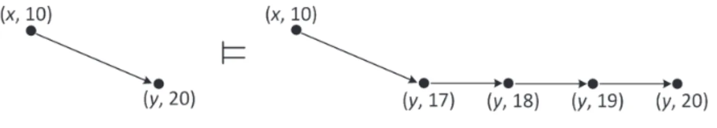
ofGT-Maxsatisfyu−t >DISTx,y then we insert a node (x,u−DISTx,y), and split the arc(x∗,y∗)into two arcs((x,t), (x,u−DISTx,y)), and((x,u−DISTx,y), (y,u)). Flow vectorhis updated accordingly (see Fig. 5).

Once this has been done, we consider, for any stationx, all nodes(x,t)ofGT-Maxwhich have been created this way, add nodes(x,0)and(x,T-Max), and rank all those nodes through increasing t values (t0 = 0, . . . ,tI = T-Max). Then we replace arcs ((x,t), (x,u−DISTx,y,))by arcs((x,ti), (x,ti+1))Inand((x,ti), (x,ti+1))Out,i =0, . . . ,tI−1,

and distribute in a natural way all flow valuesh(x,t),(x,u), u > t, previously obtained,

between arcs ((x,ti), (x,ti+1))In and((x,ti), (x,ti+1))Out. We do it in a way which is

consistent with both capacitiesCAPandC, and which minimizes the sum of flow values h on the arcs((x,ti), (x,ti+1))In. Finally, we remove nodesDepot1andDepot2, and

as-sign flow values to arcs(s, (x,0))and arcs((y,T-Max),p)in such a way relations (E10, E11) of theNetwork-Flow-VSRmodel be satisfied. By doing this, we turnh into a flow vector f, which may be considered as defined on an implicit representation ofGT-Maxand which satisfies (E7, E11) of theNetwork-Flow-VSRmodel. We check that the resulting coste ∈ ET-Max fe.Vehicle-Coste only differs from initialarcs eCVe.he by the time vehiclesspend inside thecarrierson arcs((x,ti), (x,ti+1))In.

Figure 5–Decomposing an arc((x,10), (y,20))such that DISTx,y =7.

– Step 6: Construction of flow vectorF

We complete the construction of step 5 by introducing nodes(Depot,0),(Depot,T-Max)