BRUNO PETRATO BRUCK
CONTRIBUTIONS TO THE SINGLE AND MULTIPLE
VEHICLE ROUTING PROBLEMS WITH DELIVERIES
AND SELECTIVE PICKUPS
Disserta¸c˜ao apresentada `a Universidade Federal de Vi¸cosa, como parte das exigˆen-cias do Programa de P´os-Gradua¸c˜ao em Ciˆencia da Computa¸c˜ao, para obten¸c˜ao do t´ıtulo de Magister Scientiae.
VI ¸COSA
MINAS GERAIS − BRASIL
Ficha catalográfica preparada pela Seção de Catalogação e Classificação da Biblioteca Central da UFV
T
Bruck, Bruno Petrato, 1988-
B888c Contributions to the single and multiple vehicle routing 2012 problems with deliveries and selective pickups / Bruno Petrato
Bruck. – Viçosa, MG, 2012.
viii, 78f. : il. (algumas col.) ; 29cm.
Orientador: André Gustavo dos Santos.
Dissertação (mestrado) - Universidade Federal de Viçosa. Referências bibliográficas: f. 75-78
1. Pesquisa operacional. 2. Otimização combinatória. 3. Logística. 4. Otimização matemática. I. Universidade Federal de Viçosa. Departamento de Informática. Programa
de Pós-Graduação em Ciência da Computação. II. Título.
`
A minha fam´ılia, principalmente `a minha m˜ae por todo o apoio e suporte. Aos meus amigos pela boa amizade, pelo apoio e pelas horas de lazer.
Ao meu orientador Andr´e por todo o apoio, amizade, dedica¸c˜ao e por `as vezes ficar at´e de madrugada online fazendo revis˜oes comigo nos artigos para n˜ao perder o deadline.
Ao professor Arroyo pela amizade e por ajudar com o projeto para a bolsa de mestrado, sem a qual ficaria complicado continuar o mestrado.
`
A professora Luciana e ao Anand que acabaram por ajudar na decis˜ao de qual problema abordar no mestrado.
`
A Deus acima de tudo por todas as oportunidades. ...
INDEX
LIST OF FIGURES iv
LIST OF TABLES vi
LIST OF ABBREVIATIONS viii
ABSTRACT ix
RESUMO x
1 Introduction 1
1.1 Motivation . . . 3
1.2 Contributions . . . 3
1.3 Chapters . . . 4
2 Literature review 5 2.1 MILP Formulations . . . 8
2.1.1 S¨ural-Bookbinder . . . 9
2.1.2 Gribkovskaia-Laporte-Shyshou . . . 12
3 Methodology for the SVRPDSP 15 3.1 Solution representation . . . 15
3.2 Constructive Heuristics . . . 16
3.2.1 TspBased . . . 16
3.2.2 TspKnapsackBased . . . 18
3.2.3 nearestNeighbor . . . 19
3.2.4 cheapestInsertion . . . 19
3.3 Repair and improvement heuristics . . . 19
3.4 Neighborhood Structures . . . 20
3.4.1 2-Opt . . . 20
3.5 Evolutionary Algorithm . . . 22
3.6 Variable Neighborhood Descent . . . 28
3.7 A Branch&Cut for the Gribkovskaia-Laporte- Shyshou formulation . . 29
3.8 A novel MILP formulation . . . 31
3.8.1 The proposed four-commodity network flow formulation . . . . 33
4 Methodology for the MVRPDSP 37 4.1 Solution representation . . . 37
4.2 Constructive Heuristic . . . 38
4.2.1 Clustering phase . . . 38
4.2.2 Routing phase . . . 40
4.3 MILP formulations . . . 41
4.3.1 S¨ural-Bookbinder based formulation . . . 41
4.3.2 Four-commodity network flow formulation . . . 44
5 Computational Tests 47 5.1 Benchmark instances . . . 47
5.2 Parameter calibration . . . 48
5.3 Experimental results for the SVRPDSP . . . 51
5.3.1 Metaheuristics . . . 52
5.3.2 MILP formulations . . . 56
5.4 Experimental results for the MVRPDSP . . . 64
6 Conclusions and Further investigations 70 6.1 Publications . . . 72
Bibliography 74
LIST OF FIGURES
1.1 Examples for the SVRPDSP and the MVRPDSP . . . 2
(a) Example of the SVRPDSP . . . 2
(b) Example of the MVRPDSP . . . 2
3.1 Example of solution for the SVRPDSP and its representation. . . 16
3.2 Flowchart of the constructive heuristic tspBased . . . 18
3.3 Example of a 2-opt neighbor generation. . . 21
3.4 Example of a Swap neighbor generation. . . 21
3.5 Example of a k-or-opt neighbor generation with k= 2. . . 22
3.6 Example the structure of patternsList. . . 26
3.7 Example of a crossover iteration. . . 27
3.8 Example of the shrink process. . . 32
3.9 Route passing through customers j; i; k. . . 32
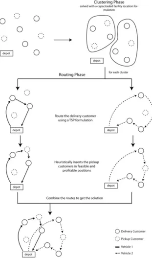
4.1 Example of solution for the MVRPDSP and its representation. . . 38
4.2 Example of how the constructive heuristic for the MVRPDSP works . . . . 39
5.1 ANOVA of the constructive heuristics tspBased and tspKnapsackBased . . 49
5.2 Graph showing the gap values for the constructive heuristics tspBased(rclSize = 1) and tspKnapsackBased(rclSize={1,2}) . . . 50
5.3 ANOVA of the EA parameters . . . 50
5.4 Graphs for the Analysis of Variance of therclSizeof the hybrid constructive for the MVRPDSP . . . 52
(a) ANOVA for all instances . . . 52
(b) ANOVA for instances of size 72 . . . 52
5.5 Average gapvalues per instance type . . . 55
(a) Considering the best gap values . . . 55
(b) Considering the average gap values . . . 55
5.7 ANOVA of the normalized lower bound values of the three formulations for the SVRPDSP. . . 61
LIST OF TABLES
5.1 Best solutions of our approaches compared to the ones from the literature . 53 5.2 Average solutions of our approaches compared to the ones from the literature 54 5.3 Comparison of the Algorithms with the literature considering the average
gap(%) for instances with typep two excluding instance 076 B half . . . 55 5.4 Results of the S¨ural-Bookbinder formulation for the SVRPDSP . . . 58 5.5 Results of the proposed four-commodity network flow formulation for the
SVRPDSP . . . 59 5.6 Comparison of the number of best solutions, optimals and proved optimals
found by the exact approaches for the SVRPDSP . . . 60 5.7 Comparison of the solution values and computational times from the
for-mulations for the SVRPDSP . . . 62 5.8 Comparison between the solutions found by the metaheuristics and the
op-timals proved by the formulations. . . 63 5.9 Results of the proposed formulation for the MVRPDSP based on the one
from S¨ural and Bookbinder [30] with and without initial solution . . . 67 5.10 Results of the proposed four-commodity network flow formulation for the
MVRPDSP with and without initial solution . . . 68 5.11 Comparison of the proposed approaches for the MVRPDSP . . . 69
AC Additional constraints
ANOVA ANlysis Of VAriance
AS Anti-symmetry constraints
CC Constraint Disaggregation and Coefficient Improvement
CI Cover Inequalities
CVRP Capacitade Vehicle Routing Problem
EA Evolutionary Algorithm
GA Genetic Algorithm
GVNS General Variable Neighborhood Search
ILP Integer Linear Programming
ILS Iterated Local Search
KC Knapsack Constraints
LB Lower Bound
LC Lifted capacity constraints
LI Logical Inequalities
LS Lifted MTZ Subtour Elimination Constraints
MACS Multi-ant Colony System
MILP Mixed Integer Linear Programming
MTZ Miller-Tucker-Zemlin Constraints
MVRPDSP Multiple Vehicle Routing Problem with Deliveries and Selective Pickups
RCL Restricted Candidate List
SVRPDSP Single Vehicle Routing Problem with Deliveries and Selective Pickups
TS Tabu Search
TSP Traveling Sallesman Problem
VND Variable Neighborhood Descent Algorithm VRPB Vehicle Routing Problems with Backhauls
VRPDP Vehicle Routing Problems with Deliveries and Pickups
VRPSPD Vehicle Routing Problem with Simultaneous Pick-up and Delivery services
ABSTRACT
BRUCK, Bruno Petrato, M.Sc., Universidade Federal de Vi¸cosa, October 2012.
Contributions to the Single and Multiple Vehicle Routing Problems with Deliveries and Selective Pickups. Adviser: Andr´e Gustavo dos Santos. Co-adviser: Jos´e Elias Claudio Arroyo.
The Single Vehicle Routing Problem with Deliveries and Selective Pickups (SVR-PDSP) is a variation of the classical Vehicle Routing Problem (VRP) that has received limited attention. It has many practical applications in reverse logistic contexts, such as in drink factories, which besides having to supply stores and supermarkets with full bottles, have to pickup empty bottles, returning them to the factory in order to be clean and refilled. There is also the Multiple Vehicle Routing Problem with Deliv-eries and Selective Pickups (MVRPDSP), which shares the same applications of the SVRPDSP. It is even more practical, since in real world cases it is commom having multiple vehicles. However, regarding the MVRPDSP, to our knowledge, there is not a single approach in the literature. In the present work, for the SVRPDSP, in terms of heuristic approaches, we propose a Hybrid Evolutionary Algorithm (EA) which makes use of a data mining strategy in its crossover and mutation phases; and a Variable Neighborhood Descent Algorithm (VND). In addition we also propose a Branch&Cut algorithm for an exact formulation of the literature and a novel formulation. Regarding the MVRPDSP we propose two formulations based on the ones of the single vehicle version of this problem and a hybrid cluster-first constructive heuristic. Experimental results show that the proposed formulation for the SVRPDSP outperforms by far the others from the literature, finding optimal solutions for more than half the instances of the benchmark used in the literature. For the MVRPDSP we created a benchmark of instances and report several good solutions, including some optimals.
BRUCK, Bruno Petrato, M.Sc., Universidade Federal de Vi¸cosa, Outubro de 2012.
Contribui¸c˜oes para o Single e Multiple Vehicle Routing Problems with
Deliveries and Selective Pickups. Orientador: Andr´e Gustavo dos Santos. Coorientador: Jos´e Elias Claudio Arroyo.
O Single Vehicle Routing Problem with Deliveries and Selective Pickups (SVR-PDSP) ´e uma varia¸c˜ao do cl´assico Vehicle Routing Problem (VRP). Tem recebido pouca aten¸c˜ao, apesar de possuir muitas aplica¸c˜oes pr´aticas em cen´arios de log´ıstica reversa, como por exemplo em f´abricas de bebidas, que ao mesmo tempo em que h´a uma demanda de supermercados e outras lojas por garrafas cheias, tamb´em existe uma demanda pela coleta de garrafas vazias a retornar para o dep´osito a fim de serem limpas e reutilizadas. Al´em disso tamb´em existe o Multiple Vehicle Routing Problem with De-liveries and Selective Pickups (MVRPDSP), o qual compartilha as mesmas aplica¸c˜oes, podendo at´e ser considerado mais pr´atico do que o SVRPDSP, j´a que em casos reais s˜ao usuais cen´arios com multiplos ve´ıculos. Entretanto, com rela¸c˜ao ao MVRPDSP n˜ao ´e de nosso conhecimento qualquer abordagem na literatura. Neste trabalho, para o SVR-PDSP, em termos de abordagens heur´ısticas, s˜ao propostos um Algoritmo Evolucion´ario H´ıbrido que faz uso de uma estrat´egia dedata mining em seus operadores de crossover e muta¸c˜ao, al´em de um Variable Neighborhood Descent Algorithm (VND). Al´em disso, tamb´em ´e proposto um Branch&Cut para uma formula¸c˜ao matem´atica da literatura e uma nova formula¸c˜ao, a qual utiliza um tipo diferente de restri¸c˜oes para elimina¸c˜ao de subciclos. Com rela¸c˜ao ao MVRPDSP, s˜ao propostas duas formula¸c˜oes matem´aticas baseadas nos modelos matem´aticos do SVRPDSP, e uma heur´ıstica construtiva h´ıbrida do tipocluster-first. Resultados experimentais indicam que a formula¸c˜ao proposta para o SVRPDSP possui um desempenho muito superior `as da literatura, conseguindo en-contrar a solu¸c˜ao ´otima para mais da metade das instˆancias. Para o MVRDPSP foram criadas instˆancias de teste e s˜ao reportados v´arios bons resultados, incluindo algumas solu¸c˜oes ´otimas.
Chapter 1
Introduction
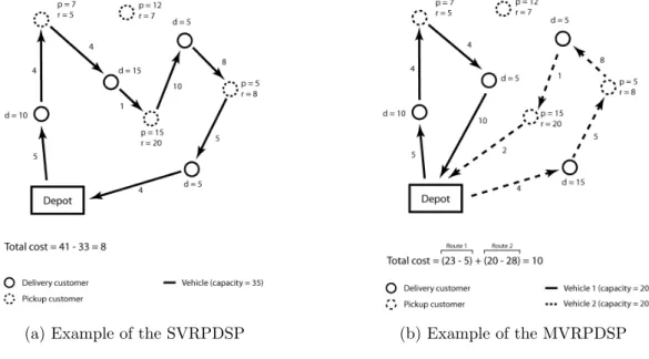
In the Single Vehicle Routing Problem with Deliveries and Selective Pickups (SVR-PDSP) there are a set of customers to be served and a depot from where a vehicle departs to serve the customers. Each customer has a certain demand of goods either to be delivered or to be picked up, which generates a revenue if collected. It is possible for a customer to have both demands. In such case, if both are going to be served, they can be performed simultaneously or in two different visits, each completely fulfilling one of the demands. The vehicle that departs from the depot shall perform a route that visits a subset of customers performing deliveries and pickups, then return to the depot. All delivery demands must be fulfilled exactly once. The pickup demands, however, are not mandatory, therefore they are only performed if there is enough space in the vehicle and if they are profitable. Serving a pickup demand is profitable if the revenue generated by collecting it is greater than the additional routing cost. One can notice that some pickups might not be served at all and it is possible to argue that they would need to be performed at some point. To address this issue these pickup demands could either be delayed to be served in the following day, or a third party service can be used to collect these pickups, which could be a less costly option than forcing all pickups to be fulfilled or sending another vehicle only to perform a few pickups. The objective is to find a route that minimizes the total routing cost, which is the travel cost to visit the customers minus the revenue generated by the collected pickups. Fig-ure 1.1a shows a small example with 8 customers and a vehicle with capacity equals to 35. In the figure, d is the delivery demand of a customer, while p stands for the pickup demand and r is the revenue generated by performing the respective pickup demand of the customer. The transportation cost of the solution presented is equal to 5 + 4 + 4 + 1 + 10 + 8 + 5 + 4 = 41 and the total revenue generated by the three pickups collected is 5 + 20 + 8 = 33. Therefore the total cost of this solutions is 41−33 = 8. In
addition notice that one pickup was not performed, which does not make the solution unfeasible, since only the delivery demands are mandatory.
Similarly there is the Multiple Vehicle Routing Problem with Deliveries and Selec-tive Pickups (MVRPDSP) which is a generalization of the SVRPDSP and only differs from it by adding the possibility of having multiple vehicles and, therefore, multiple routes. In addition we consider the fleet as homogeneous, what implies that all vehicles have the same capacity. Figure 1.1b depicts a small example with eight customers. In this example the route of vehicle 1 has a transportation cost of 5 + 4 + 4 + 10 = 23 and it generates a revenue of 5 by performing one pickup demand, therefore the total cost of this route is 23−5 = 18. The second route has a transportation cost of 20, but it generates a revenue of 8 + 20 = 28, therefore the total cost of such route is −8, which means that this route ended up generating a profit greater than its cost. Considering both routes the total cost of this solution is 18 + (−8) = 10. Notice that route 2 cannot be done in the reverse order, since there is no space in the vehicle to collect the first pickup demand as it would be still full with the delivery goods.
(a) Example of the SVRPDSP (b) Example of the MVRPDSP
Figure 1.1: Examples for the SVRPDSP and the MVRPDSP
The SVRPDSP may be conveniently described using a complete directed graph
G = {V, A}, where V = {0,1, ..., n} is a vertex set representing the depot (vertex 0) and the n customers and A ={(i, j) : i, j ∈ V, i 6=j} is a set of arcs. Each customer
i has a delivery demand di ≥ 0, a pickup demand pi ≥0, and a revenue ri ≥0. Each
arc (i, j) ∈ A has a travel cost cij. The vehicle has a capacity Q, with Q ≥
P
i∈V di.
1. Introduction 3
In order to describe the MVRPDSP, instead of considering one vehicle, letK be the set of vehicles. We assume that all vehicles inK have the same capacityQ, therefore the fleet is homogeneous. This problem is clearly NP-hard since the SVRPDSP is a special case (when |K|= 1).
1.1
Motivation
Both, the SVRPDSP and the MVRPDSP, arise in several reverse logistics contexts. An example is drink factories, which besides having to supply stores and supermarkets with full bottles, have to pickup empty bottles, returning them to the factory in order to be clean and refilled [25]. This problem also arises in logistic companies, which besides having delivery demands of packages, also have a demand of packages to be picked up that will be transported to the depot before being delivered elsewhere.
Another context is refered by [4] and [5], in which as a consequence of the constant growth in global awareness to preserve the environment, companies that manufactures electronics and batteries are being responsible to also pickup their broken and used products that otherwise would go as normal trash and pollute. For instance in Brazil, there is a law, from 2010, that entrusts companies and sellers with reverse logistic tasks related to their products, avoiding unnecessary trash being discarded and polluting the environment [18].
Regardless their many practical applications and their similarity with other ve-hicle routing problems, the literature regarding these problems is rather scarce, with only a few papers approaching the single vehicle version and none studying the multiple vehicles one.
1.2
Contributions
In this work we propose some heuristic and exact approaches for both, the SVRPDSP and MVRPDSP. For the SVRPDSP we have implemented and tested an Hybrid Evo-lutionary Algorithm (EA) and a Variable Neighborhood Descent (VND). In terms of exact approaches we propose a Branch&Cut algorithm for a formulation of the liter-ature and also a novel formulation which uses a different kind of subtour elimination constraints.
We report the results of our approaches for the SVRPDSP, including several new solutions and some new optimal solutions for the most used instances of the literature. In addition, we propose the MVRPDSP along with 72 benchmark instances, and present the solutions found by our methods.
1.3
Chapters
The present work is divided into six chapters, including this introduction. Chapter 2 provides a literature review of the problems, describing the heuristic and exact ap-proaches already proposed, including three metaheuristics and two mathematical for-mulations for the SVRPDSP. Since the MVRPDSP is a novel problem, there is no literature regarding such problem.
We have divided the methodology chapter into two different chapters to better present the proposed approaches for each problem. Therefore, Chapter 3 presents the methodology used for the SVRPDSP, including the proposed heuristics and exact ap-proaches. Similarly, Chapter 4 provides the methodology for the MVRPDSP describing the two mathematical formulations and the hybrid constructive heuristic proposed.
Chapter 2
Literature review
Both, the SVRPDSP and the MVRPDSP belong to the same family of Vehicle Routing Problems with Deliveries and Pickups (VRPDP), also commonly referred by Vehicle Routing Problems with Backhauls (VRPB), where backhaul correspond to the pickup service. According to Parragh [24], this family of problems has four classes. In the first two, customers have either a delivery or a pickup demand while in the last two customers are allowed to have both demands.
The first class is often referreded as Vehicle Routing Problem with Backhauls (VRPB). In such problem customers have either a delivery demand (linehaul) or a pickup demand(backhaul). However all delivery demands must be performed before the pickup demands, thus mixed load are not allowed at any point. This constraint is important when the vehicles are rear-loaded and the rearrangement of the loads at the customers is not deemed feasible, as stated by Goetschalckx and Jacobs-Blecha in [13]. The multiple vehicle variant of this problem is the most studied in the literature, approached in several papers. Brand˜ao in [3] proposed a Tabu Search (TS), and Ganesh and Narendran proposed a constructive heuristic and a Genetic Algorithm (GA) in [12]. In addition, in 2009, Gajpal and Abad [11] have presented a Multi-ant Colony System (MACS). Recently Zachariadis and Kiranoudis have developed an effective local search approach in [32]. Some authors have also approached the VRPB with time windows constraints. Among the approaches for this variant are an Insertion Based Ant System proposed by Reimann et al. in [26] and a heuristic based on Large Neighborhood Search, proposed by Ropke and Pisinger in [27].
In the other hand the second class allows mixed loads, while constrainting cus-tomer to have only one type of demand, either delivery or pickup. In the literature there are several approaches for both, the single and the multiple vehicle. Recently, for the single vehicle version, Dumitrescu et al, in [8], have proposed a Branch&Cut
rithm. An Ant Colony System was proposed by Falcon et al [9]. The later considers only one commodity. For the multiple vehicle case we cite an integrated construction-improvement heuristic, by Nagy and Salhi[22].
The third class describes contexts where customer have both types of demand and can be visited twice, thus it is not mandatory to perform both demands simultaneously. Although all delivery and pickup demands must be performed until the end of the route, most of the approaches for this class in the literature allows demands to be partially performed at each visit. This class is not heavily studied in the literature, however all approaches for the second class are valid for this class if each demand is modeled as two different customers, one for the delivery demand and the other for the pickup demand, considering a transportation cost between them as zero.
Finally, in the fourth class, customers may have both demands but may be visited only once. This includes maybe one of the most studied problems the Vehicle Routing Problem with Simultaneous Pick-up and Delivery services (VRPSPD). In such problem every customer has both demands and the pickup services are not optional. In addition, a customer must be visited only once, therefore both demands must be satisfied in a single visit to the customer. This problem has been studied by a number of authors. Most approaches are heuristics including a Tabu Search (TS), proposed by Montan´e and Galv˜ao [21], a hybrid metaheuristc proposed by Zachariadis [33]. Recently, Sub-ramanian et al proposed a Parallel heuristic [29] using VND. There is also a variant of the VRPSPD, including time windows for the customers and consequently increasing the complexity of the problem. For such problem, Boubahri et al in [2] proposed an Ant Colony System and, recently Mingyong and Erbao [20] proposed a Differential Evolution Algorithm.
Notice that although our problems can be considered as VRPDP problems, none of these classes include them, since in all of them the pickups are mandatory. Therefore we suggest a new class, where customers are allowed to have only one demand or both, there are no order in which the services must be performed and the pickups are optional. In the suggested fifth class, that includes both problems approached in this work, there is also the Vehicle Routing Proble with Deliveries, Selective Pickups and Time Windows. This problem only differs from the MVRPDSP by adding the time windows for the customers, which constraints the time in which a customer can be visited by the vehicle, thus increasing the complexity of the problem. To our knowledge, the only approach in the literature for this problem is a Branch&Price algorithm, proposed by Guti´errez-Jarpa, et al in [15].
2. Literature review 7
pickups and deliveries at customers and then return to the depot. They cite some natural extensions which have received limited attention so far. One of them is the SVRPDSP, which considers the pickups optional, but generating a revenue. Although the many practical applications there are few papers approaching the SVRPDSP and, to our knowledge, none about MVRPDSP.
Su¨ral and Bookbinder [30] are the first to directly address this problem. They present the problem using the notation α/β/γ, where α denotes the number of ve-hicles (1 for single and M for multiple), β the pickup service options (must or f ree
if the pickup is respectively mandatory or optional) and γ the precedence order for visiting the customers (prec if all deliveries must precede the pickups, or any if they can be visited in any order). While the SVRPDSP is 1/free/any, according to this notation, the MVRPDSP can be described as M/free/any. They cited papers dealing with the 1/free/prec and 1/must/any problems, and claimed to be the first to address the 1/free/any. For the multiple vehicle versions, they list papers for theM/must/prec
and M/free/prec, however no mention is made about the M/free/any, which is one of our objects of study. They propose a mixed integer linear programming formulation for the SVRPDSP along with some improvements on the constraints to strenghten the formulation, such as constraint disaggregation, coefficient improvement, cover and logi-cal inequalities, and lifted subtour elimination constraints. They modified 24 instances from the literature, with sizes of 10, 20 and 30 customers, to test their formulation. These instances were adapted for the SVRPDSP by setting some of the delivery de-mands as pickups in 3 different ways (20% of the customers reset as pickups, then 30% and 40%), generating a total of 72 instances, which were tested with some combina-tions of the formulation and the improvements resulting in about 75% of the instances optimally solved in a reasonable computational time for the best combination.
Coelho [6], in his master’s thesis, proposed a General Variable Neighborhood (GVNS) to solve the SVRPDSP. At first it solves the Travelling Salesman Problem (TSP) and the Knapsack problem for the instance and then uses their solutions to create an initial solution for a General Variable Neighborhood Search algorithm (GVNS). A theoretical lower bound is calculated in the same way as proposed by [14], using the values of the optimal solutions of the TSP and Knapsack formulations. The authors were able to significantly improve the solutions found by [14], including 3 optimal solutions as their values are equal to their respective lower bound.
Since we adapted the formulation of Sural and Bookbinder [30] to the MVRPDSP and proposed a Branch&Cut algorithm for the formulation of Gribkovskaia, Laporte and Shyshou [14], we describe them in details in the following section.
2.1
MILP Formulations
As previously stated, there are two mixed linear integer programming formulations for the SVRPDSP in the literature, while there is none for the multiple vehicle version.
Let us define the following notation, which will be used from now on to describe the input data of the problems:
• Vd: set of delivery customers
• Vp: set of pickup customers
• V: set of nodes (V =Vd∪Vp∪0)
• K: set of vehicles (|K|= 1 for the SVRPDSP)
• di: delivery demand of customeri
• pi: pickup demand of customer i
• ri: revenue associated with the pickup of customer i
• cij: cost for travelling through arc (i, j)
• D: total delivery demand (D=P
i∈Vddi)
• P: total pickup demand (P =P
i∈Vppi)
2. Literature review 9
Notice that this notation does not allow a customer to have both demands at the same time. Therefore, in such case, the customer is split into two different customers, one having the delivery demand, the other the pickup demand, and assuming a zero transportation cost between them.
2.1.1
S¨
ural-Bookbinder
This formulation, presented in [30], uses three sets of decision variables. Let xij = 1
if customer i immediately precedes customer j (i 6= j) in the route and 0 otherwise. In order to define subtour elimination constraints, let yi be the total delivery load on
the vehicle when departing from customer i. Similarly, let zi be the total pickup load
on the vehicle when arriving at customer i. Then their mathematical model for the SVRPDSP is as the following.
S¨ural-Bookbinder formulation for the SVRPDSP
M inX
i∈V
X
j∈V
cijxij −
X
i∈V
X
j∈Vp
rjxij (2.1)
Subject to: X
i∈V
xij = 1 ∀j ∈Vd∪0 (2.2)
X
j∈V
xij−
X
j∈V
xji = 0 ∀i∈V (2.3)
yi−yj ≥dj−D(1−xij) ∀i, j ∈V \ {0} (2.4)
zj−zi ≥pi−Q(1−xij) ∀i, j ∈V \ {0} (2.5)
(yi+di) + (zi+pi)≤Q ∀i∈V \ {0} (2.6)
yi, zi ≥0, xij ={0,1} ∀i, j ∈V (2.7)
the maximum capacity of the vehicle by the inequality yi+di+zi ≤ Q. Similarly, if
i is a pickup customer, the inequality yi +zi +pi ≤ Q specifies that the load of the
vehicle, when leaving customer i, must be within the capacity limit. Finally (2.7) are non-negativity and binary restrictions.
In addition S¨ural and Bookbinder proposed some improvements to strengthen their formulation and improve its efficiency, which will be described in the following.
2.1.1.1 Improvements
The set of arcs Acan be partitioned into the disjoints subsets Vd×Vd,Vd×Vp,Vp×Vp
and Vp ×Vd where C1×C2 denotes the arcs from the customer set C1 to C2. They improve the coeficients of constraints 2.4 and 2.5 resulting in the following sets.
Constraint Disaggregation and Coeficient Improvement (CC)
yi−yj ≥dj−min{D, Q−pj}(1−xij) ∀i, j∈V \ {0} (2.4.1)
zj −zi≥pi−min{P, Q−di}(1−xij) ∀i, j∈V \ {0} (2.5.1)
Note that these disaggregation will only improve the arc sets {Vd∪Vp} ×Vp in
2.4.1 and Vd× {Vd∪Vp} in 2.5.1. For constraints 2.4.1 this is valid since if the pickup
customer j is not being served in a given solutionyj = 0, the left-hand side cannot be a
negative value and, consequently, cannot be less than the value of the right-hand side. Furthermore, if j is in the solution, the smallest value the left-hand side can assume will be when i is a pickup customer not being served and yi = 0. In such case, for a
route to be feasible there must be enough space for the pickup demand of customer j
in the vehicle, therefore yj ≤ min{D, Q−pj} and the constraint remains valid. The
disaggregation in constraints 2.5.1 follows a similar idea.
These MTZ constraints can be improved even more by applying a lifting by bring-ing the variable xji into these inequalities, resulting in the following set of constraints.
Lifted MTZ Subtour Elimination Constraints (LS)
yi−yj+ [min{D−di−dj, Q−pj−di}]+xji≥dj−min{D, Q−pj}(1−xij) ∀i, j∈V \ {0} (2.4.2)
zj−zi+ [min{P, Q−di} −pi−pj]+xji≥pi−min{P, Q−di}(1−xij) ∀i, j∈V \ {0} (2.5.2)
Regarding constraints 2.4.2 the basic idea is to tight as much as possible the constraint by improving the left hand side when xji = 1, which implies that xij = 0.
For matters of simplicity, consider the term [min{D−di−dj, Q−pj−di}]+xji as T.
2. Literature review 11
Therefore, in the first case suppose that i, j ∈ Vp. Thus, yj = yi, since none of the
customers has delivery demand, and in T the resulting value will be Q−pj. One can
easily notice that in such case the left hand side will be equal to the right hand side, which satisfies the lifted constraint. The case where i, j ∈Vd can be proved to satisfy
these constraints by a similar process.
The third possible case for constraints 2.4.2, refers to wheni∈Vp andj ∈Vd. In
such case, yj = yi, the term T will result in D−dj, and the right hand side D−dj,
since D ≤ Q. Therefore the lifted constraints remain valid. Finally, there is the case in which i∈Vdandj ∈VP. Notice that the term yj−yi ≥0 and that it is equal to the
delivery demand di. Therefore if D−di ≤ Q−pj −di in term T, the constraint will
result in D ≤ min{D, Q−pj}, remaining valid. Otherwise, the constraint will result
in Q−pj ≤ Q−pj, which is also valid. Constraints 2.5.2 can be proved by a similar
process.
In order to improve the capacity constraints (2.6), consider an additional variable
qi, which assumes the value 1 if pickup i is collected and 0 otherwise.
We may define these variables by (2.8), disaggregate the constraints for delivery and pickup nodes and set the capacity to 0 if the pickup node is not visited. The capacity may be improved further using the demand of the previous and next nodes, yielding the lifted constraints (2.6.1) and (2.6.2).
Logical Inequalities (LI)
X
j
xji−qi= 0 ∀i∈V (2.8)
yi+zi+
X
j∈Vd
djxji ≤Q−di ∀i∈Vd (2.6.1)
yi+zi+
X
j∈Vp
pjxij ≤(Q−pi)qi ∀i∈Vp (2.6.2)
Note that the variable qi in (2.6.2) may be eliminated using its definition (2.8),
then none of the improvements presented so far increases the number of variables nei-ther the number of constraints of the formulation. The following additional constraints increases the size of the formulation, but can still be useful: the first is 0-1 knapsack constraints, and the second is a set of cover inequalities, which is proved by [23] to be valid inequalities for a subset K if P
Knapsack Contraints (KC) and Cover Inequalities (CI)
X
i∈Vp
piqi≤Q (2.9)
X
i∈Vp
qi≤ |K| −1 ∀K ⊆Vp,
X
i∈K
piqi > Q (2.10)
2.1.2
Gribkovskaia-Laporte-Shyshou
In this formulation, each customer i is represented by two vertices, i and i+n, but these vertices do not represent delivery and pickup. Vertices i = 1. . . n represent the first visit on customeriand verticesi+n= 1 +n . . .2n the second visit. The deliveries are performed in the first visit. The pickup may be performed simultaneously (in the first visit), separately (in the second visit) or not performed at all. Notice that this formulation assumes that all customers have both demands.
The variables xij are the same as in the previous formulation (1 if arc (i, j) is in
the route, 0 otherwise). However they are not defined for arcs (i, i+n) and (i+n, i), since if a customer is visited twice, the two visits will never be consecutive in the route. Variablesyiandzihave different meanings. They do not control the load on the vehicle:
yi = 1 if the pickup of customer i is made on a first visit, 0 otherwise; zi = 1 if the
pickup of customer i is made on a second visit, 0 otherwise. To control the load on the vehicle they introduce a new set of variables, wi, which is the upper bound on the
vehicle load when leaving vertex i.
For uniformity, we use the same notation Vd and Vp, however Vd={1. . . n} and
2. Literature review 13
Gribkovskaia-Laporte-Shyshou formulation for the SVRPDSP
M inX
i∈V
X
j∈V
cijxij −
X
i∈Vd
riyi−
X
j∈Vp
rj−nzj−n (2.11)
Subject to:
X
i∈V
xij = 1 ∀j∈Vd∪0 (2.12)
X
j∈V
xij = 1 ∀i∈Vd∪0 (2.13)
X
i∈V
xij =zj−n ∀j∈Vp (2.14)
X
j∈V
xij =zi−n ∀i∈Vp (2.15)
zi+yi ≤1 ∀i∈Vd (2.16)
0≤wi ≤Q ∀i∈V (2.17)
w0 =D (2.18)
wj ≥wi−dj+pjyj−Q(1−xij) ∀i∈V;j ∈Vd (2.19)
wj ≥wi+pj−nzj−n−Q(1−xij) ∀i∈V;j∈Vp (2.20)
X
(i,j)∈S
xij ≤ |S| −1
∀S ⊂ {V} ; 2≤ |S| ≤2n; S +{0, ..., n}
(2.21)
xij, yi, zi ∈ {0,1} ∀i, j∈V (2.22)
The objective function (2.11) minimizes the total routing cost deducting the rev-enue generated by collecting pickups. Constraints (2.12) and (2.13) imposes that the vehicle must leave the depot, visit all delivery customers only once and then return to depot. Constraints (2.14) and (2.15) assures that the route visit the customer a second time if the pickup is to be made on a second visit, otherwise the customer is not visited a second time. Constraints (2.16) guarantee that a pickup is made at most once for each customer. Constraints (2.17) control the upper bound on the load of the vehicle and constraints (2.18) set the upper bound load when leaving the depot as the total delivery demand. The set of constraints (2.19) and (2.20) defines wj in terms of wi
feasi-ble, we do not add subtour constraints for sets including all those customers. Finally, constraints (2.22) define the binary variables.
2.1.2.1 Improvements
The formulation may be strenghten through lifting process on constraints (2.19) and (2.20). The process is similar to the one presented for the MTZ constraints in the Sural-Bookbinder formulation. For example, (2.19) can be rewritten as wj ≥wi−dj+
pjyj −Q(1−xij) +αjixji, where currently αji= 0. They established the largest value
of αji so that (2.19) remains valid. This value depends if i is the first or the second
visit of the customer, and then (2.19) and (2.20) become four sets of lifted constraints. We present these improvements in the following equations.
Liftings on constraints 2.19 and 2.20
wj ≥wi−dj+pjyj −(1−xij)Q+ (Q+dj+di−pi−pj)xji ∀i∈Vd;j∈Vd (2.23)
wj ≥wi+pj−nzj−n−(1−xij)Q+ (Q+di−pi−pj−n)xji ∀i∈Vd;j∈Vp (2.24)
wj ≥wi−dj+pjyj −(1−xij)Q+ (Q+dj−pi−n−pj)xji ∀i∈Vp;j∈Vd (2.25)
wj ≥wi+pj−nzj−n−(1−xij)Q+ (Q+pi−n−pj−n)xji ∀i∈Vp;j∈Vp (2.26)
Moreover, in order to work also for the depot, before applying the lifting process, the vertex 0 is duplicated, 0 being the beginning of the route and 2n+ 1 the end, which causes minor changes on constraints from (2.23) to (2.26). The new constraints are shown in the following.
Other liftings (duplicates depot in 2n+1)
wj ≥w0−dj+pjyj−(1−x0j)Q ∀j∈Vd (2.27)
wj ≥w0+pj−nzj−n−(1−x0j)Q ∀j∈Vp (2.28)
w0≥wi+ (di−pi)x0i−(1−x0i)Q ∀i∈Vd (2.29)
w0≥wi+pi−nx0i−(1−x0i)Q ∀i∈Vp (2.30)
wj ≥w2n+1−(1−xj,2n+1)(Q+dj)−pj(xj,2n+1−yj) ∀j∈Vd (2.31)
wj ≥w2n+1−(1−xj,2n+1)Q−pj−n(xj,2n+1−zj−n) ∀j∈Vp (2.32)
Chapter 3
Methodology for the SVRPDSP
In this chapter we describe the methodology for the SVRPDSP. Since the metaheuris-tics have the same solution representation and share some procedures we first describe them. In the first section, we provide the solution representation used in our heuristic approaches. Further we describe our constructive heuristics in details, followed by a de-scription of our repair and improvement heuristics. Next, the neighborhood structures used are presented. In the following we describe the metaheuristic approaches imple-mented for the SVRPDSP, including a Hybrid Evolutionary Algorithm, which uses a data mining strategy to track good attributes of solutions and guide the crossover and mutation operators; and a Variable Neighborhood Descent. In addition we present a Branch&Cut algorithm for the formulation of Gribkovskaia, Laporte and Shyshou [14] and a novel formulation for the SVRPDSP.
3.1
Solution representation
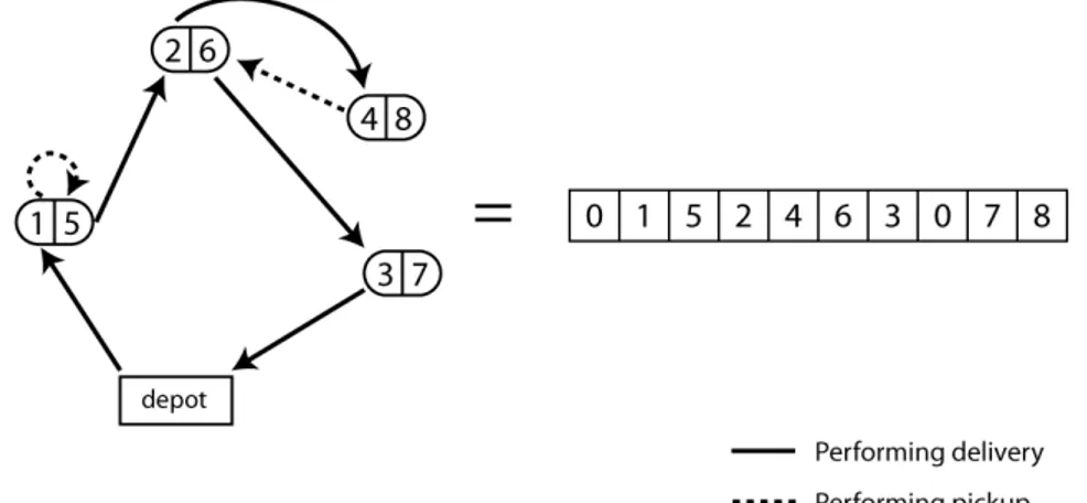
As in [6] a solution is represented by an array of integers, denoting the order in which the customers are visited. The depot is represented by the number 0 and appears twice to indicate where the route begins and where it ends. All customers that appears between the two 0’s are in the route and the remaining are customers that will not be visited. As one can notice, only pickup customers can appear out of the route as only their demands are optional.
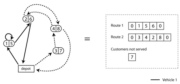
Since in our benchmark instances all customers have both demands, we assume that each customer i is represented by two different integers, i and i+n, respectively for the demand and pickup service, where n is the number of customers. Therefore solutions as the one presented in Figure 3.1 are possible and are represented as show in the same figure. Notice that as customers 7 and 8 are not being visited they appear
after the second depot in the representation, and that the demands of customer 1|5 are being performed simultaneously, while customer 2|6 has its pickup demand being performed in a second visit.
Figure 3.1: Example of solution for the SVRPDSP and its representation.
3.2
Constructive Heuristics
Four constructive algorithms were implemented, where the first two usually generate good quality solutions and the remaining two generate medium or even poor quality solutions. The only case in this work where poor quality solutions may be useful is in the EA metaheuristic, where there must be diversity among the individuals of the population.
3.2.1
TspBased
This heuristic is based on the one proposed in [6]. In this method, at first, a Traveling Salesman Problem (TSP) considering only the delivery customers is solved. The basic idea is to route these customers in the best way possible minimizing the transportation cost. Notice that the solution of this TSP is a valid solution for the SVRPDSP, since
D ≤Q, and serving the pickup customers is optional. The following TSP formulation is used and solved using the software IBM ILOG CPLEX 12.3.
M in X
i∈Vd∪0
X
j∈Vd∪0
3. Methodology for the SVRPDSP 17
Subject to:
X
i∈Vd∪0
xij = 1 ∀j∈Vd∪0 (3.2)
X
j∈Vd∪0
xij = 1 ∀i∈Vd∪0 (3.3)
X
j∈Vd∪0
(fik−fki) = 1 ∀k∈Vd (3.4)
fij ≤ |Vd|xij ∀i, j∈Vd∪0;i6=j (3.5)
xij ∈ {0,1};fij ≥0 ∀i, j∈Vd∪0 (3.6)
For this formulation consider xij = 1 if arc (i, j) is being used and 0 otherwise.
Variablesf are flow variables from network flow problems andfij defines the flow of the
arc (i, j). The objective function (3.1) minimizes the total routing cost. Constraints (3.2) and (3.3) specify that the vehicle arrives and leaves exactly once each customer. The set of constraints (3.4) defines a continuous flow throughout the route. Inequalities (3.5) specify that if arc (i, j) is used its flow must be within the total number of customers plus the depot, otherwise set the flow as zero. Finally (3.6) are non-negativity and binary restrictions.
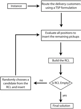
The optimal route of the TSP is used as base for inserting the pickup customers, possibly improving the current solution, which at this point only has the delivery customers being served. The insertion of the pickups is performed iteratively. At each iteration, all possible positions to insert all the remaining pickups are evaluated and the best candidates and their positions to insert stored in a Restricted Candidate List
Figure 3.2: Flowchart of the constructive heuristic tspBased
The difference between this heuristic and the one presented in [6] is the addition of a RCL, which allows different solutions to be generated when rclSize >1.
3.2.2
TspKnapsackBased
This constructive heuristic is very similar to the previous one, differing only by not considering all pickup customers in the evaluation that generates the RCL. Basically we consider only the pickup customers with the best cost-benefit and in order to discover which are these customers we solve the well known Knapsack Problem, considering the pickup customers as the items of the knapsack, their pickup demand as the weights and their revenues as the values of the items. If all pi are integers, a pseudo-polynomial
dynamic programming may be used, but for matters of generality we prefer to use a method suitable for all cases. Many other methods could be used, however the SVRPDSP instances are rather small for the Knapsack Problem, and the following simple ILP works well and is solved using the software IBM ILOG CPLEX 12.3.
M axX
i∈Vp
3. Methodology for the SVRPDSP 19
Subject to:
X
i∈Vp
pixi≤Q (3.8)
xi ∈ {0,1} ∀i∈Vp (3.9)
3.2.3
nearestNeighbor
At first the solution contains only the depot, and one by one the customers are inserted into the route. The nearest customers are inserted first. It differs from the classical nearest neighborhood heuristic by considering a RCL with size equal to 0.1n, where n is the number of customers of a given instance. Through tests it was observed that, for this problem, this algorithm yields better results the greedier it is and the value 0.1n has proven to balance well the quality and the generation of different solutions. Is is important to emphasise that the importance of this algorithm in the present work is only for generating diversity in the EA population, not necessarily good quality solutions, so further tests with the RCL size were not done.
3.2.4
cheapestInsertion
The solution has, initially, only the depot, and at each iteration a new customer is inserted in the route on a good position considering the cost-benefit criterion. For instance, if a pickup customer k is inserted between customers i and j, the impact in the solution cost is cik+ckj −cij +rk. Notice that for delivery customers the impact
is cik+ckj−cij. It uses an RCL of size 0.1n as in the nearestNeighbor heuristic.
3.3
Repair and improvement heuristics
Since solutions are frequently shaken and combined during the proposed metaheuristics, it is not uncommon that unfeasible solutions are generated. Instead of simply reject such solutions, a repair heuristic is used, what possibly improves the exploration of the search space.
customer. In case the solution is still unfeasible, the route is analyzed to find where there are pickups overweighting the vehicle, removing them from the route and thus ensuring feasibility.
As one can notice, pickup customers are frequently removed from the route in the process. But if they are removed from a position in the route because of overweighting the vehicle, maybe there is a feasible and profitable position later in the route, when more space is left by the deliveries performed. Therefore, after repairing a solution, this condition is verified and the solution may be improved.
The improvement procedure takes advantage of a certain property of the problem. For instance, in case a pickup demand is served at the position i in a given feasible route, it means that at any position greater thanithis demand can be fulfilled without making the route unfeasible, since if there was enough space to perform the pickup at that point, there will be, for certain, space for it at any time after, as the delivery load never increases along the route. Therefore if a customers’ pickup demand is performed before its delivery demand, this solution is never the optimal, since both demands can be fulfilled simultaneously with cost zero. In such cases the pickup service is moved to be made just after the delivery service of the same customer. One can easily notice that this property is only valid if there are customers with both demands, therefore if an instance is only composed by customers with either delivery or pickup demands, this procedure will not make any difference.
3.4
Neighborhood Structures
All of the proposed metaheuristics, including the Hybrid Evolutionary Algorithm uses multiple neighborhood structures. Basically, we have chosen three classical structures, 2-opt, swap and k-or-opt, which are described in the following.
3.4.1
2-Opt
3. Methodology for the SVRPDSP 21
Figure 3.3: Example of a 2-opt neighbor generation.
3.4.2
Swap
Simply swaps two randomly chosen customers from a solution. Figure 3.4 shows an example of how it works. Notice that pickup customers not being served may be included in the route since any customer in a solution can be chosen, even the depot.
Figure 3.4: Example of a Swap neighbor generation.
3.4.3
k-or-opt
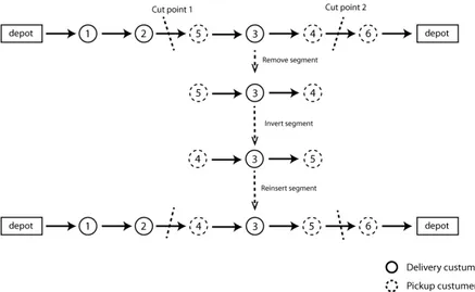
not take part on this neighborhood structure. Figure 3.5 shows an example of this neighborhood with k = 2.
Figure 3.5: Example of a k-or-opt neighbor generation with k = 2.
3.5
Evolutionary Algorithm
Basically this Evolutionary Algorithm has five distinct phases, which are the initializa-tion, crossover, mutainitializa-tion, intensification and diversification. The pseudocode 1 shows the steps of the algorithm, which are described in details in the following.
Algoritmo 1 Evolutionary Algorithm pseudocode
1: procedure Evolutionaty(popSize,numIt)
2: //Initialization 3: itsW ithoutImpr←0
4: intensity←1 // When a new best solution is found it is reset to 1
5: pop← ∅ // population
6: bestSol←any with cost =∞ // best solution 7: for i←1 to popSize do
8: constructive←random constructive heuristic
9: rclSize← random from {1,2,3}
10: Generate individual usingconstructive and rclSize
11: pop←pop∪individual
12: UpdatebestSol if necessary
3. Methodology for the SVRPDSP 23
14: Compute patternsListlist 15:
16: //EA main loop
17: for i←1 to numIt do
18: //Crossover
19: childP op← ∅
20: for j ←1 to popSize/2 do
21: parents← random 2 individuals frompop
22: //Do this for each of the 2 parents
23: child1 ← force a pattern of parents[0] into the route ofparents[1]
24: child2 ← force a pattern of parents[1] into the route ofparents[0]
25: if child1 is feasible then
26: childP op←childP op∪child1
27: UpdatepatternsListlist using child1
28: UpdatebestSol if necessary
29: end if
30: if child2 is feasible then
31: childP op←childP op∪child2
32: UpdatepatternsListlist using child2
33: UpdatebestSol if necessary
34: end if
35: end for
36: newP op←best popSize/2 from childP op∪pop
37: AddpopSize/4 from tournament(pop,childP op)
38: AddpopSize/4 random from childP op∪pop
39:
40: //Mutation
41: for j ←1 to popSize/2 do
42: individual ← random frompop 43: newM ut← mutate individual
44: Update patternsListlist using newM ut
45: Update bestSol if necessary
47: //Intensification
48: for j ←1 to popSize/5 do
49: ind← random individual from pop
50: for i←0 to intensity do
51: Shakeind
52: end for
53: ind← LocalSearch toind
54: Update patternsListlist using ind
55: Update bestSol if necessary
56: end for
57:
58: //Diversification
59: if i mod 10 = 0 then // Every 10 iterations
60: for j ←popSize−1 to popSize/2 do // Replace the worst
61: newInd← random by constructive
62: UpdatepatternsListlist using newInd
63: end for
64: end if
65:
66: if itsW ithoutImpr = 5 then 67: itsW ithoutImpr ←0 68: intensity+ +
69: else
70: itsW ithoutImpr+ +1
71: end if
72: end for 73: end procedure
In the Initialization phase, the first population is set. Each individual is gen-erated by randomly selecting a constructive algorithm among the four types available, described in details in section 3.2. In case the chosen algorithm is either tspBased or
3. Methodology for the SVRPDSP 25
this constraint. This can decrease its performance and then, should be avoided. In order to do so, if a new element is not successfully inserted into the population within 3 iterations, the value of rclSize is set as 3 increasing the chances of the constructives
tspbased ortspKnapsackBased generate a different element.
The second phase is the Crossover procedure, in which elements of the population are combined to generate new solutions so as to improve the quality of the individuals and promote, at some degree, diversification.
In order to produce better individuals the crossover procedure needs a criteria to evaluate the features of a given individual and decide which ones are the best. Therefore, before continuing explaining the crossover procedure we firstly go through the details of how our EA keeps track of good attributes of a solution.
Basically we use a Data Mining strategy, in which every new individual has its route analyzed to extract patterns (sequence of customers) within a given range [minP atternSize,maxP atternSize]. Each pattern found is stored in a structure called
patternsList along with the frequency it has appeared in the solutions already ana-lyzed. In addition to these information, we also keep record of the average cost of the route in which the pattern was found so as to improve the robustness of the eval-uation criteria that decides how good a pattern is. Therefore we have two types of data to evaluate a pattern: frequence and average cost. Good patterns have high frequency and low average cost. Since cost value is usually much higher than the frequency value, this data must be normalized. Lets call nF requency the normal-ized frequency value, nAvgCost the normalized average cost. Therefore we define
qualityIndex= (1−nAvgCost) +nF requency, as the value used to evaluate the pat-terns, since it considers both measures. The closer to 2 the better. This is not the first time an approach combining a heuristic and a data mining algorithm is proposed for a vehicle routing problem. In [28], Santos et al proposed 4 approaches for a single vehicle routing problem, including one that combines a Genetic Algorithm with the data mining algorithm Apriori. Our approach is not based on their approach and is fairly different from the algorithm they developed.
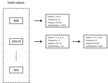
Since the number of insertions and searches through the patternsList is high, this structure is implemented as a hash table to optimize these operations. Figure 3.6 shows how this structure is organized. To describe the hash function consider
P = (c1, c2, ...cm) as a pattern, or in other words, a segment of a route; ci is a customer
andm the size of the pattern. The hash function used ishashV alueP =c1101+c2102+
..+cm10m. This hash function balances well the number of collisions and the number
of keys in the hash table, although further tests were not performed.
Figure 3.6: Example the structure ofpatternsList.
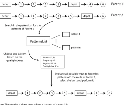
first two elements of the population are randomly selected and the patterns of both parents extracted along with their respective qualityIndex value. Let us refer to the parents asP1 andP2. One pattern ofP1 is chosen, giving more probability for the ones with higherqualityIndexvalues, and it is forced to appear in the best possible position of P2’s route generating a new individual.Then, we do the opposite, a pattern ofP2 is chosen to be forced into P1’s route. Therefore for each crossover iteration 2 children are generated. It is important to notice that in order to efficiently force a pattern, we evaluate every possibility to force a given pattern into the route and choose the best one considering the cost of the new route. However we consider only the positions where one of the customers in the chosen pattern is present. For instance, consider the route
R = (0,1,2,4,5,3,0) and the pattern P = (3,2). There are two different possibilities to force the pattern. The first one would produce the route R1 = (0,1,3,2,4,5,0) and the second R2 = (0,1,4,5,3,2,0). The crossover procedure is performed popSize/2 times in each iteration. Figure 3.7 illustrates one iteration of the process.
After the child population has been completely generated, it is time to combine it with the parent population to decide which individuals will be held for the next generation. The new population is half composed by the best elements of both popula-tions. A quarter is selected through tournaments, where the best of two elements (one from each population) wins and is inserted in the new population. The other quarter is composed of randomly selected individuals. This three stage process enhance the diversity, which is a very important factor for the success of this kind of algorithm.
3. Methodology for the SVRPDSP 27
Figure 3.7: Example of a crossover iteration.
higher the value ofqualityIndex. In case the new individual is better than the original, it replaces the latter. It is important to emphasize that, as in the crossover phase, the function which forces the patterns to appear in a given individual never generates unfeasible solutions, since it uses the repair procedure, described in section 3.3.
In the intensification phase an individual is randomly selected and its route shaken intensity times, using one of five different structures to shake a route, also randomly selected, which are 2-Opt, Swap and k-or-opt, with k ={1,2,3}, described in 3.4. Initiallyintensity= 1 and at each 5 iterations without improvement on the best solution, its value is increased by one. When the best solution is updated the value is reset to 1. A local search (Algorithm 2) procedure is then applied to the shaken individual. This procedure randomly select a neighborhood structure and completely explores it, returning the local minima. It uses the same neighborhood structures used by the shake method.
Finally the diversification phase simply replaces half of the population (the worst individuals) by new ones, generated by the constructive algorithms at each 10 iterations.
Algoritmo 2 Local Search pseudocode
1: procedure localSearch(individual)
2: neighborhood ← randomly select from {2-opt, swap, 2-Or-Opt, 3-Or-Opt,
4-Or-Opt}
3: newind← local optima ofneighborhood using individual
4: returnnewind 5: end procedure
average cost of the patterns. The earlier version used only the frequency. Besides that we propose and include the repair and the improvement procedures, which were not present in the previous EA.
3.6
Variable Neighborhood Descent
A Variable Neighborhood Descent (VND) [16] was also implemented and its steps are shown in pseudocode 3. Notice that in order to set the initial solution we run our constructive algorithms tspBased with rclSize = 1 and tspKnapsackBased with
rclSize = 1,2 and select the best solution generated. These configurations were chosen since they are the ones which generate the best solutions. Computational results to support this statement will be presented in section 5.2.
3. Methodology for the SVRPDSP 29
Algoritmo 3 Variable Neighborhood Descent pseudocode
1: procedure VND(individual)
2: bestSol←tspBased(rclSize= 1)
3: updateBestSol(tspKnapsackBased(rclSize= 1))
4: for i←1 to 5do
5: updateBestSol(tspKnapsackBased(rclSize = 2)) 6: end for
7: neighborhood←1
8: while neighborhood <6 do 9: solAux←bestSol
10: switchneighborhood
11: case 1
12: solAux← 2-opt-complete(bestSol)
13: case 2
14: solAux← swap-complete(bestSol)
15: case 3
16: solAux← 1-or-opt-complete(bestSol)
17: case 4
18: solAux← 2-or-opt-complete(bestSol)
19: case 5
20: solAux← 3-or-opt-complete(bestSol)
21: if solAux.cost < bestSol.cost then 22: bestSol←solAux
23: neighborhood←1
24: else
25: neighborhood+ +
26: end if
27: end while 28: end procedure
3.7
A Branch&Cut for the
Gribkovskaia-Laporte-Shyshou formulation
identi-fied that this formulation is much less efficient than the one proposed by Sural and Bookbinder [30]. It is clear that the subtour elimination constraints play a important role in the efficiency of this formulation. These constraints we are referring to are the following.
X
(i,j)∈S
xij ≤ |S| −1
∀S⊂ {V}; 2≤ |S| ≤2n; S+{0, ..., n}
(3.10)
One can easily notice that the number of these constraints grows exponentially to the number of customers, therefore they have a considerable impact on the efficiency of the model, even running it in commercial and very optimized softwares as IBM ILOG CPLEX.
We propose a Branch&Cut algorithm to add the subtour elimination constraints to the model as they are needed, instead of adding them all at once. This could significantly increase the performance of the model. For that end we need to be able to identify whether a given solution violates (3.10) or not, i.e., has subcycles or not. Notice that during the Branch&Cut there are two kinds of nodes: integers and fractionals. A node is integer if all x variables have integer values; and fractional if at least one x is fractional. While nodes of the former type are feasible solutions for the SVRPDSP, the latter represents only partial solutions, since some binary variables assume linear values.
Identifying subtours in integers nodes is fairly simple. Consider a given integer node ni and that the instance being solved has n customers. The formulation even
without the subtour elimination constraints enforces that a route must begin and end at the depot, therefore we are able to know how many customers are in this route by tracing it using the values of variables x. In case any delivery customer is not visited in this route we have at least two subtours and, conveniently, the route we traced to come to this conclusion is one of them. The other subtours (if there are) can be found using the same process, only changing the initial node to one that is not part of any subtour already identified.
In the other hand, the process to identify whether a fractional node has subtours is not that simple. Crowder and Padberg presents a method in [7] to identify subtours in fractional nodes of a TSP problem, which we used for the same purpose in the SVRPDSP. From now on we are going to refer to this method as the Shrink process.
3. Methodology for the SVRPDSP 31
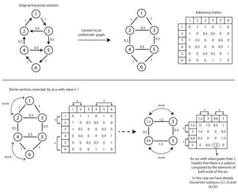
to an undirected graph. Therefore, since a solution for the SVRPDSP is represented by a directed graph, the first step is to convert it to an undirected graph.
At each iteration it is verified if there are any edges with value greater than or equal to one. In case there are, one is selected and the vertices at the ends of the edge are merged. The new vertex shares the same edges of its former vertices, therefore in case the merged vertexes were connected to a common vertex other than them, the two edges become one and their values are summed. A subtour can be identified if an edge with value greater than one is generated after shrinking. In such case there is a subtour connecting the vertices that are part of both ends. This is valid since after shrinking these vertices, the sum of the edges connecting the resulting vertex to the others will result in a value less than 2, which is a behavior that does not occur in a solution without subtours: the sum must be at least 2, since the route must arrive in at least one customer of this subset and also leave this subset at least once. Figure 3.8 depicts an example of the process. Notice that, besides the subtour constraints, this fractional solution satisfy all other constraints, including the flow constraints, as the in and out degree of each vertex sums 1. Notice that after shrinking vertices 1 and 2 an edge with value 1.5 is generated. Therefore there is a subtour connecting vertexes 1,2 and 3. This information can be used to create a cut constraint for this node, using the equations 3.10 whereS ={1,2,3}. Furthermore notice that vertexes 4,5 and 6 are also connected by a subtour. The process continues until is no longer possible to shrink the graph.
The Branch&Cut algorithm implemented uses these two methods to analyze each node generated in the branching tree, be it an integer node or a fractional one. In case the node has subtours, a cut for each subtour is generated using equations 3.10 and added to the model. Therefore, the optimal solution found in the end of the run will not contain subtours even without adding all possible subtour elimination constraints.
3.8
A novel MILP formulation
Figure 3.8: Example of the shrink process.
carries a total of exactly n units.
Similarly, for the CVRP, considering a demand di for each customer i, let
D = P
idi be the vehicle capacity. The vehicle departs fully loaded, with D units
of commodity A, drops the demand at each customer visited and ends the route with 0 units. While doing the tour, it collects di units of commodity B at each customer,
ending up with D units of commodityB. Notice that while the load of commodityA
decreases, commodity B increases by the same amount. Then, commodity B may be viewed as the free space on vehicle, since on each arc the total load of both commodities combined is exactly D. Letfij and gji be respectively the vehicle load of commodityA
and the free space when travelling through arc (i, j). Notice that the indices in g are reversed, as the free space (or commodity B) increases while following the same tour, but in the reverse order.
3. Methodology for the SVRPDSP 33
Figure 3.9 shows a general example of a subtour using variablesf and g, passing through three customers. Notice that equations (3.11) and (3.12) are valid, and we can prove the following lemma from them:
fji−fik =di (3.11)
gki−gij =di (3.12)
Lemma 3.8.1. For each customer i, the difference between the total value of the in-coming and outgoing arcs are exactly 2di.
Proof. Without lost of generality consider the customer i of Figure 3.9. Arcs not used in the tour have f =g = 0, then the incoming arcs sumfji+gki and the outgoing arcs
sum fik+gij. Using (3.11) and (3.12) we have:
(fji+gki) - (fik+gij) = fji−fik+gki−gij = 2di
This property is used in the following formulation we propose for the SVRDSP.
3.8.1
The proposed four-commodity network flow formulation
As in the formulations of Sural-Bookbinder (section 2.1.1) and Gribkovskaia-Laporte--Shyshou (section 2.1.2) we use the variable x to control which arcs are being used in the route. Therefore let xij = 1 if arc (i, j) is used and 0 otherwise. Inspired by the
two-commodity network flow formulation for the CVRP previously mentioned we use variablesf andg to control the load on the vehicle on each arc. Since we have delivery and pickup demands, we actually propose a four-commodity network flow formulation. Then let fd
ij and gjid be the delivery load and free space, respectively, when travelling
through arc (i, j), and fijp and g p
ji be the pickup load and free space, respectively. It
is important to notice that free space here is considered separately for delivery and pickup demands, i.e., pickup demands actually uses the free space of delivery load and vice-versa, although the delivery demands can be different from the pickup demands.
Variables fd are similar to the y variables of the Sural-Bookbinder formulation,
but represents the load of anarcbeing traversed, not upon departure of a vertex. They can be related by the expression yi =P(i,j)∈Afijd. Similarly,fp variables are related to
the z variables of the Sural-Bookbinder formulation. Therefore we use variablesf and
g to control the flow of load, avoiding subtours.
The four-commodity network flow formulation for the SVRPDSP
M in X
(i,j)∈V
cijxij−
X
(i,j)∈V
rjxij (3.13)
Subject to: X
i∈V
xij = 1, ∀j ∈Vd (3.14)
X
i∈V
xij ≤1, ∀j∈Vp (3.15)
X
j∈V
xij −
X
k∈V
xki= 0, ∀i∈V (3.16)
fijd +fijp ≤Qxij, ∀i, j∈V (3.17)
fijd +gjid =Qxij, ∀i, j∈V (3.18)
fijp +gjip =Qxij, ∀i, j∈V (3.19)
X
j∈V
fjid +gijd
−X
j∈V
fijd+gdji
= 2di, ∀i∈Vd (3.20)
X
j∈V
fjip +gijp−X
j∈V
fijp +gpji= 2pi
X
j∈V
xij, ∀i∈Vp (3.21)
xij ∈ {0,1}, ∀i, j∈V (3.22)
fijd, fijp, gdji, gpji≥0, ∀i, j∈V (3.23)
The objective function (3.13) minimizes the total route cost deducting the rev-enue generated by collecting pickups. The route must visit exactly once each delivery customer (3.14) and may visit at most once the pickup customers (3.15). By con-straints (3.16) each arrival produces a departure. The set of concon-straints (3.17) limits the combined amount of delivery and pickup load on each arc: the vehicle capacity if the arc is used, and zero otherwise. Constraints (3.18) and (3.19) define g’s variables in terms of f’s variables. Constraints (3.20) and (3.21) assures Lemma 3.8.1 respectively on delivery and pickup customers. For pickup customers the lemma holds only for the ones visited; for the non visited the load flow is zero. Finally, constraints (3.22) and (3.23) define the variables. In this formulation, subtour elimination is implicitly considered in the load flow variables f and g.
3.8.1.1 Improvements on the formulation
Coefficients of constraints (3.17) may be slightly improved if node i is a delivery cus-tomer and/or node j is a pickup customer. If i is a delivery customer, then the total load when leaving i cannot exceed Q−di, since di units of demand were dropped at
3. Methodology for the SVRPDSP 35
cannot exceed Q−pj, as pj units will be collected at customer j. Combining both
cases, we have the following improvement in the coefficients.
Coefficient Improvement on capacity constraints (CI)
fijd +fijp ≤(Q−max(di, pj))xij, ∀i, j∈V (3.17.1)
Consider a customeri having delivery and pickup demands at the same time. In such case, as explained in section 2.1, this customer would be split into two customers, one with each demand. Therefore there are two different ways of performing both demands simultaneously (in a single visit), first the delivery demand and then the pickup or the opposite. As one can notice, it makes no difference the order these demands are fulfilled, disconsidering feasibility. However the model considers each possibility as a different solution with same cost value.
In our test problems all customers have both demands, so the number of solu-tions with this kind of symmetry is exponential, thus we propose the following set of constraints (3.24) to remove this symmetry by not allowing a pickup demand to be performed just before the delivery demand of the same customer. Then, if they are to be served simultaneously, the route in the model visits the split customers serving the delivery and then the pickup demand consecutively, not the opposite. Notice that, because of the vehicle capacity, we cannot force the opposite, since being feasible to perform the delivery and then the pickup does not imply that the opposite would also be feasible. This is the case when the pickup demand collected occupies the free space left by the delivery goods dropped.
Anti-symmetry constraints (AS)
xi+n,i= 0 ∀i∈Vd (3.24)