Abstract
Increased demands on the capacity of the railway network gave rise to new issues related to the dynamic response of railway tracks subjected to moving vehicles. Thus, it becomes important to evaluate the applicability of traditionally used simplified models which have a closed form solution. Regarding simplified models, transversal vibrations of a beam on a visco-elastic foundation subjected to a moving load are considered. Governing equations are obtained by Hamilton’s principle. Shear distortion, rotary inertia and effect of axial force are accounted for. The load is introduced as a time varying force moving at a constant velocity. Transversal vibrations induced by the load are solved by the normal-mode analysis. Reflected waves at the extremities of the full beam are avoided by introduction of semi-infinite elements. Firstly, the critical velocity obtained from this model is compared with results of an undamped Euler-Bernoulli formulation with zero axial force. Secondly, a finite element model in ABAQUS is examined. The new contribution lies in the introduction of semi-infinite elements and in the first step to a systematic comparison, which have not been published so far.
Keywords: transversal vibration, moving load, moving mass, dynamic stiffness matrix, semi-infinite elements, critical velocity, finite element model.
1 Introduction
Railway transportation is faster, safer, more comfortable and less pollutant, when compared with road traffic. Therefore the European railways are facing the challenge of tailoring the railway system for the 21st century in order to improve their competiveness with airway transport. It is necessary to have an efficient computational tool giving quick response with sufficient accuracy to the arising questions. At this point it is necessary to evaluate the applicability of traditionally used simplified models which have a closed form solution. Simplified models have
Critical Velocity obtained using Simplified Models of
the Railway Track: Viability and Applicability
Z. Dimitrovová and A.F.S. Rodrigues
UNIC, Department of Civil Engineering
Universidade Nova de Lisboa, Portugal
in B.H.V. Topping, J.M. Adam , F.J. Pallarés, R. Bru, M.L. Rom ero, ( Edit ors) , " Proceedings of t he Tent h I nt ernat ional Conference on Com put at ional St ruct ures Technology" , Civil- Com p Press, St irlingshire, UK, Paper 36, 2010.
many advantages: (i) only the main results are available, so they are simple to analyse; (ii) the results preserve parameter dependence, allowing for direct sensitivity analysis; (iii) numerical evaluation can be carried out only in places of interest. Due to the simplifying assumptions, however, it must be stressed that the results obtained correspond only to an estimate of the structural response to a moving load. Therefore it is necessary to know to what extent these results can be utilized.
Regarding simplified models addressed in this contribution, transversal vibrations of a beam on a visco-elastic foundation subjected to a moving load are considered. Theory of small displacement is implemented. Governing equations are obtained by Hamilton’s principle. Shear distortion, rotary inertia, effect of axial force and material damping are accounted for. All characteristics of the system are assumed as piece-wise constant. “Zones” are defined as the longest possible parts of the structure where all these values are constant. It is assumed that if the full structure is finite, then it is composed by a finite number of zones. The load is introduced as a time varying force moving at a constant velocity. Transversal vibrations induced by the load are solved by the normal-mode analysis. The natural frequencies are obtained numerically exploiting the concept of the global dynamic stiffness matrix. This ensures that the frequencies obtained are accurate.
If an infinite structure is under consideration, it is necessary to remove the effect of the supports: mitigate the perturbation by the boundary conditions themselves and prevent reflection of travelling waves. For this purpose, two ways are suggested. Firstly [1], a “region of interest”, i.e., a part of the full structure where the results are supposed to be analysed, has to be defined. The initial zone will be enlarged, the moving load will actuate further from the extremity and the load value will smoothly increase from zero to its full value along a “transition” region. A procedure for estimation of the length of such transition region is presented. This approach does not bring additional computational cost, because all expressions are analytical and can be evaluated only within the region of interest. Secondly, reflected waves at the extremities of the full beam are avoided by introduction of “semi-infinite zones”. This is a new contribution, which was not published before. Introduction of semi-infinite zones is not straightforward, because the corresponding stiffness matrix is complex, even for undamped Euler-Bernoulli formulation. Semi-infinite zones are added to the structure extremities. Vibration modes are defined and determined as undamped, in the real domain. Possible norm ensuring modes orthogonality is defined. After that complex parts of the stiffness matrix are added as concentrated dampers. This impossibilitates uncoupling of the generalized displacement. Results are presented and verified.
The paper is organized in the following way. In Section 2 governing equations and their solution for the most general case of transversal vibrations in beams is presented and the differences and errors in natural frequencies are analysed. In Section 3 the concept of the global dynamic stiffness matrix is explained and the rules for the numerical expression of the results are established. Then material damping influence is discussed and differences between piece-wise continuous and discrete foundation are highlighted. After that the methodology described in [1] is briefly reviewed and infinite zones are defined, introduced and justified. In Section 4 summary of the achievements and further challenges are stated. The work presented should help in decisions concerning simplifying assumptions in problems related to dynamics of railway tracks.
2 Problem Statement
2.1 Governing Equations and Problem Solution
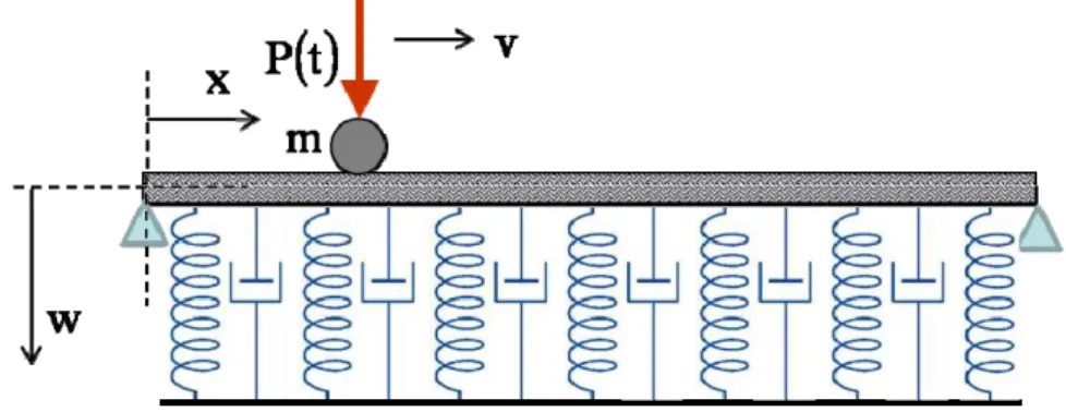
Let a uniform motion of a time variable vertical load along a horizontal finite beam on a linear visco-elastic foundation be assumed (Fig. 1). The foundation is modelled as a set of distributed springs and dashpots.
Figure 1: Simply supported beam on visco-elastic foundation.
Let the natural frequencies and vibration modes be addressed first. Hamilton’s principle is used to derive the governing equations. The potential energy U of the homogeneous beam on elastic foundation reads as:
∫
= ⎟⎟⎠ ⎞ ⎜
⎜ ⎝ ⎛
+ ⎟ ⎠ ⎞ ⎜ ⎝ ⎛
∂ ∂ + ⎟ ⎠ ⎞ ⎜
⎝ ⎛
∂ ∂ − ψ +
⎟ ⎠ ⎞ ⎜ ⎝ ⎛
∂ ψ ∂
= L
0 x
2 2 2
2
dx kw x
w N x w A
G x EI 2
1
U (1)
and the kinetic energy T as:
∫
= ⎟⎟⎠ ⎞ ⎜
⎜ ⎝ ⎛
⎟ ⎠ ⎞ ⎜ ⎝ ⎛
∂ ∂ ρ + ⎟ ⎠ ⎞ ⎜ ⎝ ⎛
∂ ψ ∂ ρ
= L
0 x
2 2
dx t w A t
I 2
1
where EI and AG stand for the bending and the shear stiffness, ρ is the density, A and I stand for the area and the moment of inertia of the transversal section of the beam. N is the axial force and k is the Winkler constant. w(x,t) and ψ(x,t) are the vertical displacement and the bending rotation; x is the spatial coordinate and t is the time. L corresponds to the total beam length. It is convenient to use the mass per unit length μ=ρA and substitute ρI by μr2, where r is the radius of gyration.
It holds for the dynamic equilibrium:
( ) 2
(
U T)
dt 0 1t
t
1 − =
δ
∫
, (3)where δ( )1 is the first variation. By integration by parts and by taking into account general statement for boundary conditions, it yields for the terms in the potential energy: dt dx kww w x w N x x w A G w x w A G x x EI x 2 1 t t t L 0 x ⎟ ⎟ ⎠ ⎞ ⎟⎟ ⎠ ⎞ − ⎟ ⎠ ⎞ ⎜ ⎝ ⎛ ∂ ∂ ∂ ∂ + ψ ⎟ ⎠ ⎞ ⎜ ⎝ ⎛ ⎟ ⎠ ⎞ ⎜ ⎝ ⎛ ∂ ∂ − ψ − ⎜ ⎜ ⎝ ⎛ ⎜⎜ ⎝ ⎛ ⎟ ⎠ ⎞ ⎜ ⎝ ⎛ ⎟ ⎠ ⎞ ⎜ ⎝ ⎛ ∂ ∂ − ψ ∂ ∂ − ψ ⎟ ⎠ ⎞ ⎜ ⎝ ⎛ ∂ ψ ∂ ∂ ∂ −
∫ ∫
= = (4)and in the kinetic energy:
∫ ∫
= = ⎟⎟⎠ ⎞ ⎜⎜ ⎝ ⎛ ⎟ ⎠ ⎞ ⎜ ⎝ ⎛ ⎟ ⎠ ⎞ ⎜ ⎝ ⎛ ∂ ∂ μ ∂ ∂ + ψ ⎟ ⎠ ⎞ ⎜ ⎝ ⎛ ∂ ψ ∂ μ ∂ ∂ − 2 1 t t t L 0 x 2 dt dx w t w t t rt . (5)
Grouping the corresponding terms, two governing equations for free vibrations are obtained: 0 t r x w A G x EI x 2 2 2 = ∂ ψ ∂ μ − ⎟ ⎠ ⎞ ⎜ ⎝
⎛ −ψ ∂ ∂ + ⎟ ⎠ ⎞ ⎜ ⎝ ⎛ ∂ ψ ∂ ∂ ∂ , (6) 0 t w c kw x w N x x w A G x t w 2 2 = ∂ ∂ + + ⎟ ⎠ ⎞ ⎜ ⎝ ⎛ ∂ ∂ ∂ ∂ − ⎟ ⎠ ⎞ ⎜ ⎝ ⎛ ⎟ ⎠ ⎞ ⎜ ⎝
⎛ −ψ
∂ ∂ ∂ ∂ − ∂ ∂
μ . (7)
. 0 t w c kw x w N t w t A G r x A G EI 1 x t w r x w EI 2 2 2 2 2 2 2 2 2 2 2 4 2 4 4 = ⎟⎟ ⎠ ⎞ ⎜⎜ ⎝ ⎛ ∂ ∂ + + ∂ ∂ − ∂ ∂ μ ⎟⎟ ⎠ ⎞ ⎜⎜ ⎝ ⎛ ∂ ∂ μ + ∂ ∂ − + ∂ ∂ ∂ μ − ∂ ∂ (8)
Assuming harmonic vibration by circular frequency ω,
( )
( )
i t e x w t , xw = ω , one can determine the corresponding mode shape from:
(
)
(
ic k)
w 0A G r 1 EI 1 dx w d k ic A G 1 N A G N 1 r EI 1 dx w d A G N 1 2 2 2 2 2 2 2 2 4 4 = − ω − μω ⎟⎟ ⎠ ⎞ ⎜⎜ ⎝
⎛ −μ ω − + ⎟⎟ ⎠ ⎞ ⎜⎜ ⎝ ⎛ − ω − μω + ⎟ ⎠ ⎞ ⎜ ⎝ ⎛ − ⎟ ⎠ ⎞ ⎜ ⎝ ⎛ + ω μ + ⎟ ⎠ ⎞ ⎜ ⎝ ⎛ + (9)
implying the equation for complex wave numbers as: 0 B Ap
p4+ 2+ = , (10)
where ⎟ ⎠ ⎞ ⎜ ⎝ ⎛ + ⎟⎟ ⎠ ⎞ ⎜⎜ ⎝
⎛ ⎟+μω − ω−
⎠ ⎞ ⎜ ⎝ ⎛ − ⎟ ⎠ ⎞ ⎜ ⎝ ⎛ + ω μ = A G N 1 / A G k ic N A G N 1 r EI 1 A 2 2
2 , (11)
(
)
⎟ ⎠ ⎞ ⎜ ⎝ ⎛ + − ω − μω ⎟⎟ ⎠ ⎞ ⎜⎜ ⎝⎛ −μ ω − = A G N 1 / k ic A G r 1 EI 1 B 2 2 2 . (12)
Four complex wave numbers correspond to each natural frequency, in the form of:
B 2 A 2 A p 2
1 ⎟ −
⎠ ⎞ ⎜ ⎝ ⎛ − −
= , B
2 A 2 A p 2
3 ⎟ −
⎠ ⎞ ⎜ ⎝ ⎛ + −
= , (13)
B 2 A 2 A p 2
2 ⎟ −
⎠ ⎞ ⎜ ⎝ ⎛ − − −
= , B
2 A 2 A p 2
4 ⎟ −
⎠ ⎞ ⎜ ⎝ ⎛ + − −
= . (14)
Thus
2 2
2
1 B p
2 A 2 A i B 2 A 2 A
p ⎟ − =−
⎠ ⎞ ⎜ ⎝ ⎛ + = − ⎟ ⎠ ⎞ ⎜ ⎝ ⎛ − −
= . (15)
( )
∑
= = 4 1 j x p j j e C xw ,
( )
∑
= = ψ 4 1 j x p j j j e q C
x , (16)
where
(
+μω − − ω)
+
= Np k ic
p A G
1 p
q 2 2
j j j
j , j=1,…,4. (17)
Consequently the bending moment is given by:
∑
= − = ∂ ψ ∂ − = 4 1 j x p j j j j e q p C EI x EIM (18)
and the shear force by:
(
)
⎟⎟ ⎠ ⎞ ⎜⎜ ⎝ ⎛ − = ∂ ∂ + ⎟ ⎠ ⎞ ⎜ ⎝⎛ −ψ ∂ ∂ =
∑
= 4 1 j x p j j j j e q p C A G x w N x w A GV , (19)
which can be rewritten as:
(
)
(
)
(
)
[
+ + + − ψ]
+
= EIqq Cpe C pe q q C p e C p e N
A G
N 1
1
V 1 3 1 3 p1x 3 1 p3x 2 4 2 4 p2x 4 2 p4x (20)
permitting to simplify for zero shear deflection. Natural frequencies can be obtained by application of the boundary conditions on Eq. (9), which for the case presented in Fig. 1 are:
( )
0 0w = , w
( )
L =0,( )
0 dx x d 0 x = ψ =,
( )
0dx x d L x = ψ = . (21)
Formulation shown has several advantages, but also disadvantages. First of all to determine a significant number of complex natural frequencies is not a simple task. In addition, vibration modes of complex frequencies are not orthogonal, which makes the mode superposition method impracticable for continuous structures.
When solving vibrations induced by the moving load, right hand side of Eq. (8) must be altered as:
where P stands for the travelling force and m for the mass of the load; w and P are considered positive when acting downwards. Further in Eq. (22): v is the constant velocity and δ is the Dirac function. x has its origin at the left extremity of the structure, as shown in Fig. 1. Zero time corresponds to force position at x=0. Initial conditions are given as:
( ) ( )
x,0 F xw = ,
( )
G( )
xt t , x w
0 t
= ∂
∂
=
. (23)
In cases when Eq. (22) can be solved by normal-mode analysis [2-3], deflection is assumed in form of:
( )
x,t q( ) ( )
tw xw j
1 j
j
∑
∞ == . (24)
where qj
( )
t are the generalized displacements and wj( )
x are the orthonormal natural modes normalised by:( )
x dx r( )
x dxw
N 2 2j
L
0 2
j L
0
j=
∫
μ +∫
μ ψ . (25)2.2 Natural
Frequency
Comparison
Firstly, commonly used simplifications in already simplified models are evaluated. At this point it is possible to compare the natural frequency. In analytical approach, the influence of the rotary inertia and of the shear deflection with respect to the Euler-Bernoulli formulation is analyzed. Then comparison with finite element software is performed. The effect of the visco-elastic foundation and of the axial force will be neglected for now. 100m long simply supported beam in form of two standard UIC60 rails will be taken as a case study. Table 1 summarizes the input data.
Property Beam (2 UIC60)
Young’s modulus E (GPa) 210
Poisson’s ratio 0.3
Density ρ (kg/m3) 7800
Transversal section area A (m2) 153.68·10-4 Coefficient of area reduction 0.41
Moment of inertia I (m4) 6110·10-8
Bending stiffness EI (MNm2) 12.831
Shear stiffness GA (MN) 508.92 Mass per unit length μ (kg/m) 119.8704
From Table 1 moreover ρI=μr2=0.47658 kgm. Numerical solution of exact analytical formulation in Maple [4] is compared with the analytical value of the Euler-Bernoulli beam
μ ⎟ ⎠ ⎞ ⎜ ⎝ ⎛ π =
ω EI
L j 2
j in Fig. 2. Last frequency presented is extremely high, but the graphs indicate that the difference in results tends to increase substantially. In fact the number of modes is not very high and is common in realistic high-speed lines application.
Figure 2: Natural frequencies of Euler-Bernoulli formulation (red line), with influence of the rotary inertia (blue line) and with the effect of the shear deflection
(violet line).
In graph of Fig. 2 it is seen that especially the effect of the shear deflection (the violet curve) is dominating. The curve corresponding to both effects is almost coincident with the violet one. Regarding the finite element results, it is known that in the standard finite element codes higher natural frequencies are not accurately evaluated, [5]. This error cannot be solved by refining the mesh, because it is inherent to the standard finite element formulation that makes use of cubic Hermite shape functions for the beam elements. The analysis presented in [5] does not account for rotary inertia, neither for the shear deflection, which is important in higher frequencies as shown in Fig. 2.
analytical value is plotted against the n/N, i.e. in the way presented in [5], thus n stands for the mode number and N for the total number of degrees of freedom plus 1. Even if the firstly mentioned method experiences spurious modes and frequencies, the optical branch was not detected in results comparison. On the other hand it is seen that invariancy in Fig. 3b) is approximately maintained, as pointed out in [5].
Figure 3: Error analysis of numerical values with consistent mass matrix implemented (red, green, yellow, and blue lines stand for 250, 500, 1000 and 5000
elements implemented, respectively).
The error in frequencies of the flexural modes obtained in ANSYS reaches 40% as predicted in [5] for lumped mass approach. In this case the error-lines do not have the same tendency and are not invariant with respected to the ratio n/N. There is also significant error in fundamental frequency for high number of elements, namely
% 17
− for 5000 elements implemented.
The effect of an elastic foundation was tested as well. It was found that the error in natural frequencies is basically independent on the value of the foundation stiffness. However, first modes sequence is disordered, due to very proximate numerical values, even with consistent mass matrix implemented. The higher the Winkler constant, the larger the number of modes that are disordered, as it is obvious from the analytical formula for the Euler-Bernoulli beam
a)
μ + μ ⎟ ⎠ ⎞ ⎜ ⎝ ⎛ π =
ω EI k
L j 4
j . For instance when the foundation stiffness of 100 MN/m
2 is implemented, the first five mode shapes are interchanged, as it is shown in Fig. 5.
Figure 4: Error analysis of numerical values with lumped mass matrix implemented (red, green, yellow, and blue lines stand for 250, 500, 1000 and 5000
elements implemented, respectively).
It can be concluded that differences in results occur in analyses requiring large number of modes, which is very common in high-speed lines applications, because large number of modes is necessary when relatively strong foundation is implemented and/or when abrupt changes in foundation are present. Abrupt changes in foundation stiffness can be originated by geotechnical conditions, by track degradation or by alterations of the structural design. Such situations may occur in embankment-to-bridge or tunnel transitions, when passing from ballasted to slab tracks and in regions where the railways cross underground structures, thus the stiffness changes can be quite sharp.
This section justifies that finite element method can yield errors in places where they are not predictable. Therefore: i) it is important to continue with analytical solutions and use them as benchmark problems; ii) it is necessary to establish a
a)
range of validity of simplified models, because their results are obtained faster and in a more accurate way, than the ones obtained by standard finite element codes.
Figure 5: Disorder in natural modes of simply supported beam on elastic foundation, results obtained in ANSYS.
There are several ways of possible comparison. One of then is critical velocity comparison in systems with non-homogeneous foundation. Then in the validation process of simplified models the following issues has to be solved: i) what terms from the general formation are really necessary; ii) can the real discrete foundation be substituted by the continues one; iii) how to remove reflecting waves; iv) is the mass of the load important, and if yes, how to associate a mass in the foundation; v) are the results meaningless because in fact the foundation should be tensionless?
After solving issues i)-iv) in analytical way, the critical velocity of the most adequate simplified model can be compared with the full finite element analysis to validate the issue v). Some of the results are presented in the following section.
3 Simplified Models
3.1 Dynamic
Stiffness
Matrix
within each zone. Let the full structure be separated into n zones. The local dynamic stiffness matrix of s-th zone can be calculated in the following way. Its degrees of freedom are shown in Fig. 7a). Excitation with unit amplitude and given circular frequency ω is assumed in direction of one of the degrees of freedom while the other degrees of freedom are kept fixed. For such excitation, member-end generalized harmonic forces in the steady-state regime (shown in Fig. 2b) are calculated. The procedure is repeated for the other degrees of freedom. The dynamic stiffness matrix is a symmetric 4x4 matrix. For Euler-Bernoulli formulation is given for instance in [1-2, 7-8].
Figure 6: Beam structure in form of two zones.
Figure 7: a) Degrees of freedom and b) member-end generalized harmonic forces of the s-th zone with nodes i and k.
The global dynamic stiffness matrix is assembled by the direct stiffness method and its determinant is set to zero. The roots of this equation, ωj, are the natural frequencies. Substituting ω=ωj back into the global matrix, unknown nodal displacements and rotations can be evaluated.
Numerical cautions are important. Let us assume a left cantilever in the Euler-Bernoulli formulation and neglect for simplicity the mass of the load, the visco-elastic foundation and the axial force. Characteristic equation reads as:
0 1 cosh
cosλ λ+ = , (26)
where λ/L is the wave number and L is the cantilever length. The unnormalized mode shape is given by:
ik M
ki M
ik
V Vki
i s−thzone k
b) a)
i
ψ
k
ψ
i
Δ
k
Δ
( )
( )
( )
( )
( )
( )
( )
( )
( )
x .L cosh cosh cos sinh sin x L sinh x L cos cosh cos sinh sin x L sin x w j j j j j j j j j j j j j ⎟⎟ ⎠ ⎞ ⎜⎜ ⎝ ⎛ λ λ + λ λ + λ + ⎟⎟ ⎠ ⎞ ⎜⎜ ⎝ ⎛ λ − ⎟⎟ ⎠ ⎞ ⎜⎜ ⎝ ⎛ λ λ + λ λ + λ − ⎟⎟ ⎠ ⎞ ⎜⎜ ⎝ ⎛ λ = (27)
It is possible to simplify the displacement amplitude at the free end to:
( )
( )
( ) ( )
( )
j j j j j sin sinh sinh sin 2 L w λ − λ λ λ= . (28)
Numerical test in Maple software shows, that the formulation in Eq. (27) leads unexpected errors and should be rewritten to:
( )
( )
( )
( )
( )
x .L cos cosh x L cosh cos x L cosh x L cos x L sin sinh x L sinh sin sinh sin 1 x w j j j j j j j j j j j j j j j ⎟⎟ ⎠ ⎞ ⎟⎟ ⎠ ⎞ ⎜⎜ ⎝ ⎛ λ λ + ⎟⎟ ⎠ ⎞ ⎜⎜ ⎝ ⎛ λ λ − ⎟⎟ ⎠ ⎞ ⎜⎜ ⎝
⎛λ −λ − ⎟⎟ ⎠ ⎞ ⎜⎜ ⎝
⎛λ −λ + ⎜⎜ ⎝ ⎛ ⎟⎟ ⎠ ⎞ ⎜⎜ ⎝ ⎛ λ λ − ⎟⎟ ⎠ ⎞ ⎜⎜ ⎝ ⎛ λ λ − λ − λ = (29)
The numerical test results are summarized in Table 2. 20 digits precision and 100 digits precision was implemented. Differences are significant from 13th mode.
Mode number λ
Eq. (27) 100 dig Eq. (28) 100 dig Eq. (29) 100 dig Eq. (27) 20 dig Eq. (28) 20 dig Eq. (29) 20 dig 11 32.99 2.00000 2.00000 2.00000 2.00000 2.00000 2.00000 12 36.13 -2.00000 -2.00000 -2.00000 -2.00000 -2.00000 -2.00000 13 39.27 2.00000 2.00000 2.00000 1.99800 2.00000 2.00000 14 42.41 -2.00000 -2.00000 -2.00000 -2.00000 -2.00000 -2.00000 15 45.55 2.00000 2.00000 2.00000 1.00000 2.00000 2.00000 16 48.69 -2.00000 -2.00000 -2.00000 0.00000 -2.00000 -2.00000 17 51.84 2.00000 2.00000 2.00000 0.00000 2.00000 2.00000 18 54.98 -2.00000 -2.00000 -2.00000 0.00000 -2.00000 -2.00000
Table 2: Numerical precision test.
very large numbers turned out to be essential in natural vibrations calculation, which is considered the most difficult part of the numerical assessment of the results. This difficulty is aggravated by the fact, that very high number of natural frequencies is required in problems dealing with several zones. The determinant has many singularities coincident with all natural frequencies of each zone considered separately. In order to avoid special treatment around the singularities, it is possible to solve the roots only in the numerator.
3.2 Damping
The damping is addressed through the damping coefficient c in Eq. (22). It corresponds to the material damping, but it can adopt several interpretations. It is necessary to analyze carefully what is the most adequate representation in high-speed lines applications. It can be assumed c=αμ+β for convenient Rayleigh coefficients α and β, expressing mass damping of the rails and stiffness damping of the foundation. Moreover, c can be interpreted as frequency dependent or not. Damping effect in form of damping ratio ξ as a part of the critical damping was analyzed in [8]. For the sake of simplicity only Euler-Bernoulli formulation without axial force was considered and mass of the load was neglected. Then the loading term corresponds to p
( ) (
x,t =δ x−vt) ( )
P t . According to the normal-mode analysis general steps, superposition is done for undamped modes and the loading function is expanded in series as:( )
x,t( ) ( ) ( )
x Q tw xp j
1 j
j
∑
∞ =μ
= . (30)
( )
tQj is calculated by exploiting the orthonormality of the mode shapes:
( )
=∫
L( ) ( )
0
j
j t px,t w x dx
Q . (31)
Functions from the initial conditions given in Eq. (23) must be expanded in series as well. Expressions obtained can be substituted into the governing equation (22), simplified in the way specified above. Then the equation of motion in principal coordinates is deduced as:
( )
t 2 q( )
t q( )
t Q( )
tq&j + ξωj&j +ω2j j = j
& , (32)
which can be solved by Laplace transformation (* stands for the transform):
( )
( )
( )
( )
( )
( )
( )
2( )
j j 2 * j j j j j * j 2 p p Q 0 q 2 0 pq 0 q p q ω + ξω + + ξω + += & . (34)
Rewriting the denominator in the form of:
(
)
(
) (
)
2dj 2 j 2 2 j 2 j 2 j j 2 p 1 p 2
p + ξω +ω = +ξω +ω −ξ = +ξω +ω , (35)
where ωdj stands for the j-th damped frequency, it finally yields:
( )
( )
(
)
(
( )
( )
) (
)
( )
(
)
, p 1 p Q p 1 0 q 0 q p p 0 q p q 2 dj 2 j dj dj * j 2 dj 2 j dj dj j j j 2 dj 2 j j j * j ω + ξω + ω ω + ω + ξω + ω ω + ξω + ω + ξω + ξω + = & (36)which can be easily transformed back:
( )
( )
( )
( )
( )
( )
( )
( )(
(
)
)
. d t sin e Q 1 t sin e 0 q 0 q t cos e 0 q t q dj t t 0 j dj dj t dj j j j dj t j j j j j τ τ − ω τ ω + ω ω + ξω + ω = τ − ξω − = τ ξω − ξω −∫
& (37)According to Eq. (31) and definition of the Dirac function:
( )
( ) ( )
(
) ( ) ( )
( ) (
t x vt) ( )
w x dx P( ) ( )
t w vtP dx x w t P vt x dx x w t , x p t Q j L 0 j L 0 j L 0 j j = − δ = − δ = =
∫
∫
∫
(38)the final expression can be given as:
( )
( )
( )
( )
( )
( )
( ) ( )
( )(
(
)
)
. d t sin e v w P 1 t sin e 0 q 0 q t cos e 0 q p q dj t t 0 j dj dj t dj j j j dj t j j j j j τ τ − ω τ τ ω + ω ω + ξω + ω = τ − ξω − = τ ξω − ξω −∫
& (39)3.3 Discrete versus Continuous support
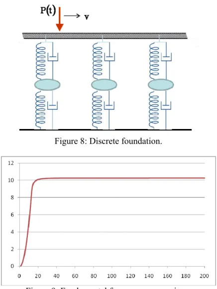
As mentioned in Section 2.2, it is important to verify, if the real discrete foundation can be substituted by the continuous one. The discrete foundation would allow for additional effects introduction, like separation of the rail pads and ballast damping, introduction of sleepers mass, etc., as it is shown in Fig. 8.
Figure 8: Discrete foundation.
Figure 9: Fundamental frequency comparison.
these models were compared. In Fig. 9 fundamental frequency is plotted. It is seen that it stabilizes on the analytical value of the continuously supported beam 10.297Hz very quickly. Realistic number of springs assuming the sleepers distance from 0.6 to 0.65m is 154-167.
3.4 Reflecting
waves
In this section, a technique which allows obtaining results within the region of interest as if were calculated on infinite beams is reviewed. The initial zone is enlarged, the moving load is let to actuate further from the zone extremity and the load value is let to smoothly increase from zero to its full value along a transition region. Thus, the length of the initial zone is separated into three lengths: initial Li, transition Lc and remaining Lr, which already contain a part of the region of interest. This separation does not bring additional computational cost, because all expressions are analytical and therefore can be evaluated only within the region of interest. The time variation of the force is assumed to have a sinusoidal shape in order to keep the time derivatives continues. In more detail:
( )
⎪ ⎪ ⎪ ⎩ ⎪ ⎪ ⎪ ⎨ ⎧
+ >
+ ≤ < ⎟
⎟ ⎠ ⎞ ⎜
⎜ ⎝ ⎛
⎟⎟ ⎠ ⎞ ⎜⎜
⎝ ⎛
⎟⎟ ⎠ ⎞ ⎜⎜
⎝ ⎛
− − π +
≤ =
v L L t for P
v L L t v L for 2
1 L L L
vt sin 1 2 P
v L t for 0
t P
c i 0
c i i
c i
c 0
i
(40)
where P0 is the final value of the force applied. This technique ensures that the maximum displacement smoothly increases until reaching its final value, which corresponds to the analytical maximum of the quasi-stationary regime. Li and Lc can be determined from analogy with a representative discrete spring. More details and results verifications are presented in [1].
3.5 Semi-infinite
Zones
letting their length tend to infinity. In summary, for semi-infinite zones tending to the left and right, respectively:
[ ]
(
)
(
)
(
)
(
)
(
)
⎥ ⎥ ⎥ ⎥ ⎦ ⎤ ⎢ ⎢ ⎢ ⎢ ⎣ ⎡ − − − − − − − − − + − − + = − 3 1 3 3 1 1 3 1 3 1 3 1 3 1 3 1 3 1 3 1 1 3 3 1 s q q p q p q EI q q p p q q EI q q q q A G p p N A G q q p q p q N A GK , (41)
[ ]
(
)
(
)
(
)
(
)
(
)
⎥ ⎥ ⎥ ⎥ ⎦ ⎤ ⎢ ⎢ ⎢ ⎢ ⎣ ⎡ − − − − − − − + − + − − − + = + 4 2 4 4 2 2 4 2 4 2 4 2 4 2 4 2 4 2 4 2 4 2 2 4 s q q p q p q EI q q p p q q EI q q q q A G p p N A G q q p q p q N A GK . (42)
These matrices are presented in [9] but their numerical implementation is not solved, which is the difficult part, because matrices in Eqs. (41-42) contain complex terms even in cases without damping. This implies complex frequencies and vibration modes related to complex frequencies are not orthogonal. We concluded and justified, that natural modes can be determined when only the real part of these matrices is assumed. After that the complex part can be implemented in form of discrete dampers. This procedure is verified on Euler-Bernoulli left cantilever without the visco-elastic foundation, with zero axial force and with neglected mass of the load. The real semi-infinite structure is modelled by two zones: one is finite (clamped on the left-hand side) with length of L0=100m, the other one is semi-infinite tending to the right. Results obtained are compared with very long cantilever of 1000m length. Results on the first 100m of the 1000m and 2000m long left cantilevers were compared and verified as coincident, in order to justify, that 1000m is sufficient to represent first 100m length of the real semi-infinite structure. Implementing the simplifications, p2 =−iλ~ and p4 =−λ~, where 4
2
EI ~= μω
λ . Therefore:
[ ]
(
)
(
)
( )
( )
⎥ ⎦ ⎤ ⎢ ⎣ ⎡ + λ λ λ − λ − = ⎥ ⎦ ⎤ ⎢ ⎣ ⎡ + − + − = + i 1 ~ ~ i ~ i i 1 ~ EI p p p p p p p p p p EI K 2 2 3 4 2 4 2 4 2 4 2 4 2s . (43)
(
)
( )
(
)
( )
( )
,dx x dw -~ 0 w 3 ~ 4 dx x L w
dx x w Re dx x L w N
2
0 x cj 2
j 2 cj 3
j 0
L 0
2 cj
0 2 sj 0
L 0
2 cj j
0 0
⎟ ⎟ ⎠ ⎞ ⎜
⎜ ⎝ ⎛
⎟⎟ ⎠ ⎞ ⎜⎜
⎝ ⎛ λ λ
μ − +
μ =
⎟ ⎠ ⎞ ⎜
⎝ ⎛ μ +
+ μ
=
= −
∞ −
∫
∫
∫
(44)
where parts of the mode shape wcj and wsj correspond to the shape definition within the cantilever and within the semi-infinite zone, respectively. The finite cantilever is assumed to have negative x coordinate, therefore the “connection” between the finite and the semi-infinite zone is at position x=0. Coordinate shift in wcj is not important for the norm evaluation, but it should be used for the mode shapes visualization. The first four normalized undamped modes are shown in Fig. 10.
Figure 10: The first four normalized undamped modes.
The problem arises in localized dampers introduction, because then equations determining the generalized displacements are coupled. They can be written in the following form:
( )
t C q( ) ( )
t ~q t Q( )
tq& + ⋅& + =
& , (45)
where ~q
( )
t is a column vector of components ω2jqj( )
t , Q( )
t is defined as in Section 3.2 by Eq. (38) and C matrix is a full square symmetric matrix of components in the form:0 x cj ci
i i cj ci i 2 i cj ci
i 2 i cj ci i 3 i ij
dx dw dx dw ~
dx dw w ~ w dx dw ~ w w ~ EI C
= ⎟⎟ ⎠ ⎞ ⎜⎜
⎝ ⎛
ω λ + ω
λ + ω
λ + ω
λ
It is thus impossible to apply Laplace transformation like in Section 3.2. Nevertheless, it is possible to solve Eq. (45) numerically. Even if it is not possible to present the result in an analytical form, these results are important, because they have not been published before. The procedure allows for exact and complete removing of the reflected waves. Fig. 11 justifies that the deflection (in mm) under the unit moving force (P=1N) within the first 100m is the same in both situations described above, i.e. in finite 100m cantilever with semi-infinite zone and in very long cantilever. Differences in results are attributed to the fact, that only 14 modes were implemented for calculation of results according to Eq. (45). This completes the verification.
Figure 11: Verification of the semi-infinite zone.
4 Conclusions and Further Development
In further development a systematic comparison, as outlined in this paper, will be continued. It will especially be directed to the critical velocity comparison. Preliminary results are presented in [7-8]. In non-homogeneous case the critical velocity is defined as the velocity at which vertical displacements achieve very high values. It is obtained by extracting the maximum displacement while parametrically varying the load velocity. In homogeneous case it can be related to resonant frequency and resonant velocity of finite as well as infinite beams.
5 Acknowledgements
References
[1] Z. Dimitrovová, “A General Procedure for the Dynamic Analysis of Finite and Infinite Beams on Piece-Wise Homogeneous Foundation under Moving Loads”, Journal of Sound and Vibration, 329, 2635–2653, 2010.
[2] V. Koloušek, “Dynamics in Engineering Structures”. Academia, Prague, Butterworth, London, 1973.
[3] L. Frýba, “Vibration of solids and structures under moving loads”. 3rd edition, Thomas Telford, London, 1999.
[4] Release 11 Documentation for MAPLE, Maplesoft a division of Waterloo Maple, Inc., 2007.
[5] J.A. Cottrell, A. Reali, Y. Bazilevs, T.J.R. Hughes, “Isogeometric analysis of structural vibrations”, Computer Methods in Applied Mechanics and Engineering 195, 5257-5296, 2006.
[6] Release 11.0 Documentation for ANSYS, Swanson Analysis Systems IP, Inc., 2007.
[7] Z. Dimitrovová, J.N. Varandas, “Critical Velocity of a Load Moving on a Beam with a Sudden Change of Foundation Stiffness: Applications to High-Speed Trains”, Computers & Structures, 87, 1224–1232, 2009.
[8] A.F.S. Rodrigues, Vibrações transversais em vigas finitas sujeitas a cargas móveis: Radiação de transição associada à mudança brusca da rigidez vertical de fundação, Master Thesis, Department of Civil Engineering, Universidade Nova de Lisboa, 2010 (in Portuguese).