Biomass allometry and carbon factors for a Mediterranean pine
(Pinus pinea L.) in Portugal
A. C. Correia*, M. Tomé, C. A. Pacheco, S. Faias, A. C. Dias, J. Freire,
P. O. Carvalho and J. S. Pereira
Instituto Superior de Agronomía. Tapada da Ajuda. 1349-017 Lisboa. Portugal
Abstract
Forests play an important role in the global carbon balance because they offset a large portion of the carbon dio-xide emitted through human activities. Accurate estimates are necessary for national reporting of greenhouse gas in-ventories, carbon credit trading and forest carbon management but in Portugal reliable and accessible forest carbon measurement methodologies are still lacking for some species. The objective of this study was to provide forest ma-nagers with a comprehensive database of carbon factors and equations that allows estimating stand-level carbon stocks in Pinus pinea L. (P. pinea), regardless of the tree inventory information available. We produced aboveground biomass and stem volume equations, biomass expansion factors (BEF) by component as well as wood basic density (WBD) and component carbon fraction in biomass. A root-to-shoot ratio is also presented using data from trees in which the root system was completely excavated. We harvested 53 trees in centre and south Portugal covering diffe-rent sizes (6.5 to 56.3 cm), ages (10 to 45 years) and stand densities (20 to 580 trees ha–1). The results indicate that
aboveground allometry in P. pinea is not comparable with other pines and varies considerably with stand characte-ristics, highlighting the need to develop stand-dependent factors and equations for local or regional carbon calcula-tions. BEFabovegrounddecreases from open (1.33 ± 0.03 Mg m–3) to closed stands (1.07 ± 0.01 Mg m–3) due to a change
in biomass allocation pattern from stem to branches. Average WBD was 0.50 ± 0.01 Mg m–3but varies with tree
di-mensions and the root-to-shoot ratio found was 0.30 ± 0.03. The carbon fraction was statistically different from the commonly used 0.5 factor for some biomass components. The equations and factors produced allow evaluating car-bon stocks in P. pinea stands in Portugal, contributing to a more accurate estimation of carcar-bon sequestered by this forest type.
Key words: Pinus pinea; carbon balance; climate change; biomass inventory.
Resumen
Alometría de la biomasa y factores de carbono para un pino Mediterráneo (Pinus pinea L.) en Portugal Los bosques juegan un papel importante en el balance global del carbono porque desplazan una gran porción del dióxido de carbono emitidos por actividades humanas. Se necesitan estimaciones precisas para los informes nacio-nales de los inventarios de los gases de efecto invernadero, mercados de créditos de carbono, y manejo de carbono en los bosques. Pero en Portugal todavía faltan, para algunas especies, metodologías de mediciones fiables y accesibles de carbono en los bosques. El objetivo de este estudio es proporcionar a los gestores forestales una base de datos com-pleta de los factores y ecuaciones del carbono que permitan estimar los stocks de carbono a nivel de rodal, en Pinus pinea, independientemente de la información disponible de los inventarios de árbol. Producimos ecuaciones de bio-masa del matorral, y del volumen del troco, factores de expansión de biobio-masas (BEF) por componente así como den-sidad básica de la madera (WBD) y fracción de los componentes de carbono en la biomasa. Un ratio raíz-tallo se pre-senta también utilizando datos de los arboles en los que los sistemas radicales se extrajeron completamente. Se cosecharon 53 árboles en el centro y sur de Portugal, cubriendo tamaños diferentes (6,5 a 56,3 cm), edades (10 a 45 años), y densidad del rodal (20 a 580 árboles ha–1). Los resultados indican que la alometria del sistema radical en P.
pinea no es comparable con otros pinos y varía considerablemente con las características del rodal destacando la ne-cesidad de desarrollar factores dependientes del rodal y ecuaciones para cálculos de carbono a nivel local o regional. BEFradicaldisminuye de rodales abiertos (1,33 ± 0,03 Mg m–3) a cerrados (1,07 ± 0,01 Mg m–3) debido a cambios en la
asignación de biomasa de tronco a ramas. La media de WBD es 0,50 ± 0,01 Mg m–3pero varía con la dimensión de los
* Corresponding author: [email protected] Received: 15-04-10; Accepted: 22-09-10.
Introduction
Reliable estimates of forest carbon stocks and chan-ges over time are necessary to understand the global carbon cycle and to know to what extent they contri-bute to mitigate greenhouse gas emissions. Feasible and comprehensive carbon estimates in forests are important under international commitments as the Kyoto Protocol or the United Nations Framework con-vention on Climate Change but also because there is a growing interest of enterprises and landowners in getting involved in the market opportunities available for forest carbon offset credits (Hamilton et al., 2007). The quantif ication, reporting and verif ication of carbon sequestered by forests are frequently not as transparent as it should and this has major implications on policy decisions regarding forest conservation and management (Clark et al., 2001).
Methods to assess carbon stock at stand level
Inventory-based methods are the most common for assessing forest carbon stock and changes. IPCC (2003) suggests that this can be done either by directly applying allometric models that predict tree biomass components based on field measurements of individual trees (like diameter at 1.30 m or tree height), or using multiplication factors that allow to convert or expand stem volume to the tree biomass component wanted. This involves the development of site-specific allome-tric equations requiring tree harvesting and weighting in the field, which is expensive and time-consuming. The use of existing equations comes as an alternative but potential intersite variation in wood quality and biomass allocation throughout stand maturity may introduce errors in the final estimates (Lehtonen et al., 2004). Biomass expansion factors (BEF) and/or con-version factors (CF) are the most widely used methods for biomass calculations because they readily convert, in only one step, stand volume estimates (usually avai-lable in forest inventories) in biomass or carbon. Both are multiplication factors but BEF allows to expand
growing stock volume to whole or merchantable biomass components of the stand (e.g. crown) while CF includes wood basic density (WBD) and carbon fraction conver-sions. Multiplication factors, foreseen by IPCC Good Practice Guidelines in the case where no biomass infor-mation is available, can be species-specific or represent broad species groups (see review in Somogyi et al., 2006). As is the case for generic allometric equations, they do not account for intersite variability and the mat-ching to the site under study requires previous measu-rements and tree harvesting. According to IPCC (2003), the uncertainty on using generic BEF, WBD and root-to-shoot ratios is considered to be about 30% but Ravindranath and Ostwald (2008), for example, state that the use of generic factors may produce misleading estimates with errors as large as 70%. In spite of the growing number on allometric relationships and ex-pansion factors, ecosystem specific studies continue to be important because they help to reduce this uncertainty.
Pinus pinea overview
In this paper we studied an emblematic Mediterra-nean species – pinion or umbrella pine (Pinus pinea L.), a native pine of Southern Europe covering about 650,000 ha of the Mediterranean Basin (Quézel and Medáil, 2003). The major interest of this species in Portugal is the production of edible nuts, and for that stands must be managed in a way to reach a maximum of 100 trees ha–1at the mature phase which occurs
around 30 years old. Even with a large inter-annual cone production variability, which depends on the cli-matic conditions during the 4 years cone development period, P. pinea provides higher incomes to owners be-cause pine seeds are highly prized in the international markets, much more than other forest resources (e.g. timber) (Mutke et al., 2005b). Other distinctive charac-teristic of the species is its genetic uniformity (Vendramin
et al., 2008) combined with a high level of fenotipic
plasticity (Mutke et al., 2005a). In fact P. pinea appears either in arid inland or coastal sea areas affected by salinity stress, and can potentially help mitigating
árboles y el ratio de raíz a tallo se encuentra entre 0,30 ± 0,03. La fracción de carbono fue estadísticamente diferente del factor comúnmente utilizado de 0,5 de algunos componentes de biomasa. Las ecuaciones y los factores produci-dos permiten la evaluación de los stocks de carbono en rodales de P. pinea en Portugal, contribuyendo a una infor-mación más precisa del carbono secuestrado por este tipo de bosque.
desertif ication problems in these particular areas. Drought tolerant species from Mediterranean regions like P. pinea may be interesting in a climate change scenario because they are naturally adapted to warmer climates and to water stress. Future scenarios of vege-tation distribution predict that these species may shift towards higher latitudes due to climate change (Benito Garzon et al., 2008; Ohlemuller et al., 2006) and turn out to be potentially interesting in future afforesta-tion/reforestation programs in regions becoming sus-ceptible to droughts. P. pinea stands managed in long rotations and with moderate wood productivity may also sequester large carbon stocks and contribute to mitigate greenhouse gas emissions. A carbon seques-tration simulation made by Del Rio et al. (2008) using a integrated single tree model (PINEA2) in even and uneven aged P. pinea stands over a 100-year period, estimated 1.2 to 1.5 Mg of carbon sequestered per ha and per year (MgC ha–1year–1). These values are
under-estimated since carbon accumulated in the soil was not accounted, only the annual tree growth and cone pro-duction.
The main objective of this paper is to provide the tools to help stakeholders in quantifying carbon stocks for P. pinea at stand level, regardless of the inventory information available for the site, and that can either be used for national quantifications, local studies as an alternative to the existing factors that revealed inappropriate. Biomass and volume allometric equations, biomass expansion factors, biomass and carbon con-version factors where developed for the species using destructive tree sampling.
Material and methods
Stand description, climate and vegetation
P. pinea in Portugal covers 3% of total forest area
(83,900 ha) but the area had grown 10% in the last 10 years (Tomé et al., 2007). Although occurring throughout the country, most of the area is located in the south where climate and soil allows higher commer-cial cone yield. The 17 stands used for the selection of the trees for destructive sampling are located in center and south Portugal (Fig. 1) covering most of the P. pinea distribution in Portugal. The climate is Mediterranean with a hot and dry summer, with a mean annual tempe-rature of 16°C. Average annual precipitation (1961-1990) varies slightly between stands ranging from 572
to 735 mm with more than 80% occurring between Oc-tober and April.
Stands are pure, except in one site (Pegões) in which
P. pinea is mixed with cork oak or maritime pine. The
understory consists of grazed pastures with annual C3 herbaceous plants and, in some stands, dispersed shrubs of Ulex and Cistus. Soil types ranged from sand, loamy sand and sandy loam textures, derived from sand stones sedimentary rocks. All of them are nutrient poor. The stand density ranged from 20 to 580 trees ha–1and LAI
ranged from 1.5 to 11, calculated as the sum of all side needle area in the plot (m2) to the plot area (m2) (Table 1).
Sample tree selection
A total of 53 P. pinea trees were harvested for biomass, stem volume, wood basic density and carbon in biomass analysis. The sampling was stratified by 5 cm diameter at breast height from 5 to 60 cm. Stem diameter at breast height (1.30 m) (d), tree height (h), height to the crown base (hc), crown radius (cr) were measured in each tree. Stand variables were subsequently calculated, namely stand density (N), stand basal area (G) and dominant height (hdom) (Table 1).
Figure 1. Pinus pinea distribution in Europe in 2008. Picture
adapted from Fady et al. (2004). The box in the right represents the location of the stands used for biomass harvesting in Por-tugal (in correspondence with the numbering from Table 1); the light gray represents the geographical area of the 101 pure plots inventoried. Valladolid 10°W 0° 10°E 20°E 45°N 40°N 35°N 30°N 25°N Lisbon Lisbon 5 4 3 2 1 Km 0 250 500 1,000
Aboveground biomass sampling
The main aboveground biomass components —stem wood, stem bark, branches and needles— were weight in 40 trees by harvesting and additionally other 13 where measured for volume calculations. Due to limited eco-nomic resources, the root biomass was weight by the excavation method in 6 of them. In some trees the cones had already been harvested (the harvesting period in Portugal is between 15thDecember and 31stMarch) so
cones were not used in the models. In fact, due to the importance of cone production, there are specific mo-dels already available to predict cone weight in the country (Freire, 2009). Trees were cut from the stump, and dead and living branches were separated from the stem. The stem wood identification inside the crown was sometimes difficult, since trees tend to produce bifurcations due to the lack of apical dominance. In these cases, the most vigorous branch was selected to represent this stem fraction. The stem was then frac-tioned in 2 m width logs (in small trees every 1 m) and weighted in the field. A disk was collected from the base of each log and weighted in the field and kept for laboratory determination of dry weight and for stem wood/bark proportion calculations. The cross diameters of the disks with and without bark were measured in fresh conditions for volume calculations. A systematic sam-pling approach was used to collect at least 20% of the
crown biomass choosing the 1stbranch in each group
of 5 starting from the base to the tip of the crown, for wood and needle separation. The remaining crown was weight in the field but without any component sepa-ration. Branches were divided in 3 diameter classes: less than 2.5 cm, between 2.5 and 7 cm and more than 7 cm and these fractions weight. Portable digital scales with 1 g precision were used for field weightings. For each tree component a sample of approximately 200-500 g was kept and sealed in labeled plastic bags for laboratory determination of dry weight. The biomass of each component was calculated by the product of dry weight to fresh weight ratio of the component sam-ple and the total fresh weight of the component in the tree, estimated by the proportion of the component in the total fresh weight (Porté et al., 2002; Ritson and Sochacki, 2003).
For tree volume we summed the volume calculated for each intermediate log with the Smalian formula assuming a cylinder geometric shape for the stump and intermediate logs and a cone geometric shape for the top log. On average, the separation and weighting of each tree took 2 hours with the work of 5 persons but the time spent in aboveground biomass separation varied according to the tree dimensions: the maximum was 5 hours with 7 persons for a tree with 3.5 Mg (fresh weight) and the minimum was 1 hour with 5 persons for a tree with 0.035 Mg (fresh weight).
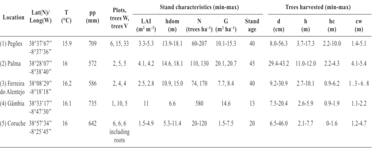
Table 1. Characteristics of the sites used for harvesting
Lat(N)/ T pp Plots, Stand characteristics (min-max) Trees harvested (min-max) Location Long(W) (°C) (mm) trees W, LAI hdom N G Stand d h hc cw
trees V (m2m–2) (m) (trees ha–1) (m2ha–1) age (cm) (m) (m) (m)
(1) Pegões 38°37’67’’ 15.9 709 6, 15, 33 3.3-5.3 13.9-18.1 60-207 10.1-15.3 40 8.0-56.3 3.7-17.3 2.2-10.0 1.4-5.1 -8°37’36’’ (2) Palma 38°28’07’’ 16 572 2, 5, 5 4.1, 4.2 14.6, 18.1 110, 130 20.1, 20.7 45 29.4-43.2 11.0-12.0 2.2-4.3 4.1-5.4 -8°38’40’’ (3) Ferreira 38°08’29’’ 16.2 586 2, 4, 4 2.5, 2.8 10.9, 15.0 74, 170 7.7, 8.4 40 9.2-30.9 2.7-10.1 0.9-6.2 1 . 3 - 6 . 8 do Alentejo -8°18’18’’ (4) Gâmbia 38°33’17’’ 16.1 735 1, 10, 5 11 6.6 580 14.6 13 7.5-20.4 2.6-5.9 0.9-1.9 1.1-2.2 -8°47’30’’ (5) Coruche 38°57’34’’ 16 642 6, 6, 6 1.5-4.9 5.3-11.4 20-120 1.5-7.5 20 6.5-46.0 2.1-7.7 0-1.6 1.2-4.7 -8°25’45’’ including roots
Climate: T, mean annual temperature (°C); pp, total annual precipitation (mm). Stand characteristics: Plots, number of plots inventoried in the stand; trees W, number of trees harvested for biomass; trees V, number of trees used for volume; LAI, leaf area
index (m2m–2); hdom, stand dominant height (m); N, stand density (trees ha-1); G, stand basal area (m2ha–1); Stand ag, of the stands.
Characteristics of the trees harvested: d, diameter at breast height (cm); h, tree height (m); hc, height to the crown base (m); cw, crown radius (m). Minimum and maximum values separated by dashes.
Root sampling
Six trees were used for root biomass determination using the excavation method. The trees were selected from stands with different soil types within the same area (Regosol, Cambisol and Luvisol) (FAO, 1998) and with different, yet low, stand densities (Table 1). After cutting the tree from the stump, a geometric polygon was identified on the ground taking into account crown projection and/or half the distance to neighborhood trees. The stump and the soil within the marked area were removed with a hydraulic excavator, and roots were separated in piles according to soil horizons and depths. The maximum depth excavated varied between 1 and 2 m according to the depth of the sandstone rock and the root system development of the tree. In each pile, roots were manually separated, washed to remove soil particles and exposed to open air to dry. The same procedure was used for the stump. Roots were sepa-rated in 3 diameter classes: less than 5 mm (fine), bet-ween 5 and 30 mm (small) and more than 30 mm (coarse), and then weighted in the field. Portable digi-tal scales with 1 g precision were used for field weigh-tings. For each tree component, two samples were collected and sealed in labeled plastic bags for dry weight and carbon analysis. All the samples were oven-dried to constant weight at 70°C for dry weight calcu-lations. The total dry biomass for each component was estimated from fresh weight based on sample dry weights.
Biomass and volume equations
The allometric relationship between tree biomass (or volume) and tree or stand variables usually takes the form of a power function and has been widely studied (see review in Zianis et al, 2005). In this study we tested the following power functions: w = kixaand
w = kixayb, where w is the dependent variable that can
be either biomass or volume, where k, a and b are parameters to be estimated by regression analysis and x and y are tree variables. The tree variables tested were: d (stem diameter at 1.3 m), h (tree height), hc (height to the crown base), cr (crown radius) and the slenderness index (h/d).
Sapwood area was also tested as a candidate ex-planatory variable. For sapwood area calculation, the surface of the disk measured at the base of the living crown was sanded on one side and then scanned on a flatbed scanner. Sapwood area and the number of rings in each disk were measured in 4 perpendicular
directions using the software WindENDRO (Regent Instruments, Sainte-Foy, Quebec, Canada). Sapwood area was only used to predict needle biomass in an independent model (following the methodology described above), since only 32 out of the 40 trees sam-pled for biomass had this measured done. These equa-tions were built because the relaequa-tionship between needle biomass (and area) to sapwood area is closely linked with plant productivity (Ryu et al., 2010) and is a common variable in carbon balance models based in the pipe-model theory (Waring et al., 1982). This theory proposes that a given unit of leaf (biomass) area is supplied with water from a constant quantity of conducting pipes and can help explain some biomass patterns in P. pinea trees with stand development.
For each component (volume with bark, stem bark, stem wood, branches and needles), the non-linear mo-dels were fitted by the least squares method, using all possible combinations of variables. The root biomass was not included in the simultaneous fit because only 6 trees were used. The performance of the biomass components models was evaluated based on the Press residuals (rp) (Myers, 1990) guaranteeing the
signifi-cance of all the parameters in the selected models. The normality of the model errors was evaluated by plotting the studentize residuals over the normal residuals (QQ-plots). The non-normality was overcome in the final model with iteratively reweighted least squares regression using the Huber function to reduce the influence of data containing large errors (Myers, 1990). To over-come heterocedasticity, the models were f itted with weighted non-linear regression, using Parresol (1999) methodology to calculate the weights. Models were evaluated using the methodology proposed by Soares
et al. (1995) and Vanclay and Skovsgaard (1997),
which consists of calculating the following statistics based on the PRESS residuals (rpi):
1) Model efficiency (Meff iciency) computed as:
where rpiis the Press residual from tree i (residual
ob-tained when tree i is not included in the fit) for the de-pendent variable, y¯ is the average value and n is the number of trees measured;
2) model bias (Mbias), expressed by the rpaverage;
3) model precision (Mprecision) expressed by the
average of the absolute values of rp. The best models
Mefficiency= 1− rpi2 i=1 n
∑
( yi− y)2 i=1 n∑
were the ones with higher eff iciency and lower bias and precision values. The models selected for each tree biomass component (except the root component), including total tree aboveground biomass expressed as the sum of the biomass components, were simultaneously f itted with the non-linear seemingly unrelated re-gression (Parresol, 1999; 2001). Model fittings where performed with SAS software (SAS, 2004).
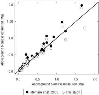
The aboveground biomass measured in the 40 trees harvested was correlated with the estimates obtained with a set of biomass equations from Spanish P. pinea stands (Fig. 1) developed by Montero et al. (2005) and the results are presented in Table 3. These consist of 7 biomass equations (for total aboveground, stem, bran-ches of less than 2 cm, between 2 and 7 cm and higher than 7 cm, needles and roots) adjusted with allometric functions using d as the independent variable. The data set used 47 trees harvested in the region of Huelva, Valladolid (Spain) (Fig. 1) with d ranging from 7.5 cm to 63 cm. No information was provided regarding stand characteristics. The average temperature (12°C) and the annual precipitation (435 mm) (1971-2000) is lower than the sites analyzed in this study probably as a result of the continental influence.
Expansion factors - biomass aboveground
and root-to-shoot ratio
To compute BEFiwe used a total of 101 pure P. pinea
permanent plots selected from a national grid (Freire, 2009) that used the same inventory methodology des-cribed in section 2.2 (Table 2). No trees were harvested from these plots, these were only used to compute BEFi. The subscript index (i) refers to needle, branches,
stem wood, stem bark, stem (wood + bark), crown (branches + needles) or total aboveground biomass, these last 3 thereafter named aggregated BEF. BEFiis
computed as follows:
Volume with bark and biomass where estimated using equations from Table 3 (presented in the Results section). BEFivalues where plotted with stand
va-riables (N, hdom and G) in order to study possible trends in biomass allocation patterns.
The root-to-shoot ratio refers to the roots and stump biomass (Mg) over total aboveground biomass compo-nents (branches, needles, stem wood and stem bark) (Mg), and was calculated for the 6 trees in which root biomass was measured.
Conversion factors - Wood basic density
(WBD) and Carbon fraction in biomass
WBD is defined here as the ratio of wood biomass (oven-dry matter) (Mg) to the green volume (m3) and
was measured in wood disks (without bark) taken each 2 m (or 1 m long) from the stem. The knots and resin wounds were separated in the disks in order to avoid local data overestimation. The displacement of volume by immersing the wood in water was the method used (Zobel and Buijtenen, 1989). Wood and bark were oven-dried until a constant weight at 60-80°C for dry weight calculations. Tree WBD was calculated by ave-raging WBD in each disk weighed by the correspon-ding diameter without bark. The variation of WBD between and within trees was f irst assessed by gra-phical analysis. Trees were grouped in 3 height classes (trees from 2 to 6 m, 6 to 10 m and higher than 10 m) and the average WBD (and the corresponding standard error) was calculated at each intermediate height (at the base, 2 m, 4 m, 6 m and so on). A regression analy-sis was then performed, using tree d, h and discs height level within the tree, as well as interactions between these variables, as regressors in order to test the signi-ficance of the effect of tree size and height level on WBD.
BEFi (Mg m−3)= Biomassi (Mg ha
−1)
Volume with barki (m3 ha−1)
Table 2. Main characteristics of the 101 Pinus pinea plots inventoried and used for BEFi
calculations and aboveground biomass calculations
N hdom G V Aboveground (trees ha–1) (m) (m2ha–1) (m3ha–1) biomass (Mg ha–1) Min 18 4 2 6 7 Mean 194 12 10 53 63 Max 1647 21 26 175 194
In order to take into account the clustered structure of the data, with correlation among consecutive observa-tions within the same tree, model error was modeled as an autoregressive process. The effect of tree size on the tree average WBD was also assessed with re-gression analysis.
A total of 70 biomass samples were collected for carbon concentration analysis. The purpose was to collect randomly 10 samples of each biomass compo-nents (needles, branches, stem bark, stem wood and roots) from different trees. However the number of samples varied due to several reasons. For roots we only used 6 trees. For needles we add 8 samples from a study carried out in the department on P. pinea. For branches we used the 10 samples collected in each of the 3 branch diameter classes described in section 2.3. For stem bark we used 6 samples because 4 out of 10 lead to inconsistent results. The method used was the dry combustion method, according to ISO Standard 10694, using a CNS elemental analyzer. To test whether the average values were signif icantly different from the commonly used 0.5 carbon fraction, we looked at the confidence interval (with 95% confidence) for each biomass component.
Stand carbon stock comparisons
From a carbon budget management perspective we may question which stands hold de maximum carbon stocks: mature stands with a few trees or young stands with high tree density? In an attempt to answer this question for the P. pinea stands in this study, we plotted stand basal area measured (G, m2ha–1) for the 101
stands inventoried, with the total carbon in the trees estimated in each stand divided in 5 stand density classes. The estimates for aboveground biomass in each stand were calculated by applying the biomass equa-tions from Table 3 (to each tree), converted in carbon using the carbon fraction for each component (from Table 5) and expressed by unit area (ha).
Results
Allometric relationships
The total aboveground biomass of sample trees varied between 20 and 1,899 kg, the branch and needle biomass ranging from 1 to 1,182 kg and from 3 to 222 kg,
Table 3. Final models selected for biomass components (in kg) and volume with bark (in m2) considering tree variables as
predictors
Equation Average Par. Estimates R2ajd M
bias Mprecision Meff iciency
(min-max) Needles k ca (h/d)b 38 (3-222) k 22.27 (18.09) 0.71 2.68 11.56 0.63 a 1.76 (1.69) (0.83) (0.97) (5.05) (0.82) b –0.50 (–0.67) Branches k ca 194 (1-1,182) k 184.94 (23.56) 0.79 1.03 66.00 0.74 a 3.03 (1.84) (0.79) (0.85) (5.89) (0.76) Stem bark k cahb 21 (1-78) k 8.08 (6.85) 0.83 0.83 4.99 0.82 a 1.55 (1.46) (0.83) (0.97) (5.05) (0.82) b 0.47 (0.54) Stem wood k cahb 154 (5-675) k 18.85 (19.26) 0.94 2.03 26.27 0.93 a 1.68 (1.61) (0.95) (2.19) (26.31) (0.94) b 0.95 (0.94) Total wl + wbr + 480 (20-1,899) k 280.1 0.92 6.57 77.27 0.91 aboveground + wb + ww a 2.33 (0.91) (10.45) (74.04) (0.91) (k cahb) b 0.19
Volume with bark k hadb 0.66 (0.02-2.73) k 0.000094
a 0.65 0.0028 0.00865 0.93
b 1.97
d: diameter at breast height (cm). c: circumference at breast height (πd/100) (cm). h: tree height (m). Average (min-max)
repre-sents the average, minimum and maximum biomass values in each biomass component used to build the models. For biomass mo-dels, the values represent the parameters and several model fitting validation tests after simultaneous fitting (in kg). In bracket the validation tests before simultaneous fitting.
respectively. The stem wood ranged from 5 to 675 kg and the stem bark from 1 to 78 kg (Table 3). The branches represented the most important fraction of the above-ground tree biomass (average 43% ± 2%) followed by the stem wood (average 37% ± 2%), needles (average 13% ± 1%) and stem bark (average 7% ± 0.3%). Diame-ter at 1.3 m (d) and height (h) were the most important independent variables in all equations and accounted for more than 71% of the variability of the different biomass components and volume equations (Table 3). Overall validation statistics with simultaneous fitting were better for branches but decreased substantially for needles remaining practically the same for stem (wood and bark) components (Table 3). The Meff iciency
for total aboveground biomass was the same for both sets (0.91), but for needle biomass equation in an inde-pendent model using sapwood area was high, sugges-ting that this variable provides a good means to predict needle biomass (Fig. 2).
For volume with bark, the values varied between 0.02 to 2.73 m2with a high M
eff iciency(n = 52).
The biomass estimates using Montero et al. (2005) equations are well correlated with the observed values (see Fig. 3). When testing the probability of the diffe-rences between variances of the two datasets we conclu-de that there are statistical differences for needles (F-test; p = 0.01 < 0.05) but not for stem and branches (p = 0.20 and 0.38). However when looking at the absolute errors
(difference between the measured and the estimated value) we observed that the estimates are quite biased. The average percentage error computed as the average of the relative error (difference between the measured and the estimated value over the measured value expressed as a percentage) for the 40 trees, resulted in an overestimation for stem and branches (22.2% and 55.3%, respectively) and a underestimation for needles of 23.4% using Montero et al. (2005) equations.
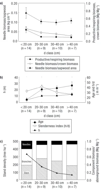
Needles/aboveground biomass tends to decrease with stand development (from 21% ± 3% at < 20 cm d class to 9% ± 3% at d > 40 cm) as well as the stem/abo-veground biomass with a minimum at d > 0 cm with 36% ± 5% (Fig. 4c). For the ratio of branches/above-ground biomass there is a tendency to increase as stands gets less denser reaching a maximum at d > 40 cm with 55% ± 4%. For trees less than 20 cm (that is young trees in dense stands), biomass allocation to the crown (and specially branches) seems to be a priority, representing more than 60% of the total aboveground biomass.
The observed decrease in the ratio of productive (needle) to respiring biomass (branches+stem wood + stem bark) as stand gets older (Fig. 4a and 4b) is rather expected (Ryan and Yoder, 1997) and is related with higher construction and maintenance respiration costs with woody tissues. Nevertheless, this decreasing rate is very smooth for d classes higher than 20 cm (average
Figure 3. Left graph: correlation between the total aboveground
biomass (Mg) measured in the 40 trees harvested and the esti-mates obtained using Table 3 equations and the biomass equa-tions for P. pinea developed by Montero et al. (2005) (in Mg).
Figure 2. Needle biomass (kg) (y) expressed as a function of
(x) that can be either d (cm) or sapwood area (cm2) measured
at the base of the live crown. Nonlinear model fitted: y = k xa.
For the f itting with: a) x = d: k = 0.06, a = 1.87, R2adj = 0.62,
Eeff iciency= 0.59, n = 40; b) x = sapwood: k = = 0.06, a = 1.08,
R2adj = 0.78, E
eff iciency= 0.70, n = 32.
Sapwood (cm2)
Montero et al.,2005 This study
d (cm) 250 225 200 125 100 75 50 25 0 2.0 1.50 1.0 0.5 0.0 0 200 400 600 800 1,000 1,200 1,400 0 10 20 30 40 50 60 d (cm) 0.0 0,5 1.0 1.5 2.0
Aboveground biomass measured (Mg)
Sapwood area (cm2)
Needle biomass (kg)
Aboveground biomass estima
12% ± 0.3%). The slenderness index was low at d < 20 cm because trees at this stand density levels invest little in height compared with diameter (Fig. 4b) and pre-sented a peak at 20-30 cm decreasing thereafter.
Expansion factors and root-to-shoot ratio
Average BEFivalues were higher for branches with
0.57 ± 0.015 Mg m–3followed by stem wood (0.42 ±
0.002 Mg m–3), needles (0.12 ± 0.005 Mg m–3) and stem
bark (0.06 ± 0.002 Mg m-3) (Table 4). The aggregated
BEFwas higher for total aboveground (1.18 ± 0.01 Mg m–3), followed by the crown (0.69 ± 0.014 Mg m–3) and
then for stem (wood + bark) (0.49 ± 0.003 Mg m–3). The
highest variability was found for BEFbranches.
Plotting the aggregated BEF with stand variables (N, G, hdom and Volume), N was the variable that pre-sented the best correlations with BEFi(Fig. 5) showing
a decreasing pattern for aboveground and BEFcrownand
an increase for BEFstem.
Maximum BEFcrownwas 1.08, decreasing to 0.41 in
very dense stands with a typical exponential decay curve shape when plotted over stand density (Fig. 5 and Ta-ble 4). The opposite is observed for BEFstemwith a
much smaller variation from 0.41 to 0.57. BEFaboveground
showed the same tendency than BEFcrown..
Regarding the root system, we observed that roots between 5 and 30 mm represents the higher fraction of the total root biomass (63%), followed by fine (20%) and coarse roots (17%). The root-to-shoot ratio found for the 6 trees harvested was 0.30 ± 0.03. The horizon-tal superficial root exploration observed in the surface layer exceeded 1.5 to 2 times the tree crown projec-tion area and about 90% of the total root biomass was in the top 50 cm. Regarding root development in depth, we also observed that f ine roots were able to penetrate in severely compacted horizons which can be extremely important for groundwater uptake in the dry season.
Table 4. Biomass expansion factors (BEFi in Mg m–3) for each
tree component (needles, branches, stem bark and stem wo-od) and aggregated BEFi (in Mg m–3) (crown, stem and total
aboveground). Columns represent the average, minimum, ma-ximum and the standard error (s.e.) for BEFi for each com-ponent. The number of plots used for BEFi calculations equals 101 (stand characteristics are described in Table 2)
BEFi Average Min Max s.e.
Needles 0.12 0.06 0.28 0.005
Branches 0.57 0.28 0.99 0.015
Stem bark 0.06 0.04 0.11 0.002
Stem wood 0.42 0.36 0.11 0.002
Crown 0.69 0.41 1.08 0.014
Stem (wood + bark) 0.49 0.41 0.57 0.003 Total aboveground 1.18 0.97 1.50 0.010
Figure 4. Average values and standard errors calculate for each
diameter at breast height class for the following variables: a) Ratio between the productive (needle) to respiring biomass
(branches + stem wood + stem bark) (Mg Mg–1); ratio between
the needle biomass to crown biomass (Mg Mg–1); ratio
bet-ween the needle biomass to sapwood area measured at the
crown base (kg cm–2). b) h: height (m); age; h/d:
height/diame-ter at 1.3 m (m m–1). c) Stand density (trees ha–1); ratio
bet-ween each biomass component to total aboveground bio-mass: Black boxes (needles), white boxes (branches), stripe bo-xes (stem). n in the axis represent the number of trees used in each class. a) b) c) 0.20 0.15 0.10 0.05 0.0 40 30 20 10 0 500 400 300 200 100 0 1.0 0.8 0.6 0.4 0.2 0.0 60 50 40 30 20 10 1.0 0.8 0.6 0.4 0.2 0.0 Needle biomass/sa pwood area (kg cm –2) < 20 cm 20-30 cm 30-40 cm > 40 cm (n = 14) (n = 9) (n = 10) (n = 7) d class (cm) < 20 cm 20-30 cm 30-40 cm > 40 cm (n = 14) (n = 9) (n = 10) (n = 7) d class (cm) < 20 cm 20-30 cm 30-40 cm > 40 cm (n = 14) (n = 9) (n = 10) (n = 7) d class (cm) h (m)
Stand density (tree ha
–1) Needles
Branches
Stem Component biomass/
aboveground biomass (Mg Mg
–1)
Age and h/d ( m m
–1)
Productive/respiring biomass, cro
wn biomass (Mg Mg
–1)
Productive/respiring biomass Needle biomass/crown biomass Needle biomass/sapwood area
Age
Slenderness index (h/d) h
Conversion factors
Wood basic density
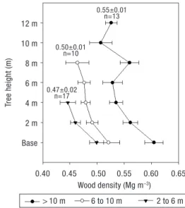
Average WBD for all trees weighted by the disks cross diameter in the stem was 0.51 ± 0.01 Mg m–3
(min-0.43 Mg m–3and max-0.60 Mg m–3). Figure 6
shows the vertical distribution of WBD in trees with different sizes. Taller trees presented the higher average values (0.55 ± 0.01 Mg m–3) and the shorter trees
showed the lowest (0.47 ± 0.02 Mg m–3). We also
obser-ved higher values in the base of the stem compared to the top. The regression analysis lead to the following model with the model error modeled as a 2ndorder
autoregressive process (all parameters signif icantly different from zero for p = 0.05):
WBD = 443.63 + 10.17 h-20.78 hi+ 20 h hi
(R2= 0.46),
where WBD is wood basic density (Mg m–3), h is tree
total height (m) and hiis height level within the tree
(m). Tree diameter at breast height, alone or combined with tree height, did not improve the model for WBD. The following model was found for tree average WBD:
WBD = 437.51 + 8.03 h (R2= 0.50),
where the symbols are as before. These analyses clearly show that WBD depends on tree height, increasing with tree size. Within the tree, WBD decreases from the soil level to the tip.
Carbon fraction in biomass
Average carbon fraction in the dry biomass for branches and roots is not significantly different from 0.5 carbon fraction (Table 5), but they are for stem wood, stem bark and needles taking into account a 95% confidence interval.
Stand carbon stock comparisons
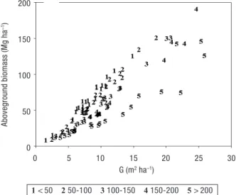
Taking into account the above methodologies, we observe in Figure 7 that the maximum carbon stock in the aboveground biomass is reached in open stands,
Figure 5. Biomass expansion factors (BEFi, Mg m–3) plotted with
stand density. Graph in the bottom: BEFcrown(branches and needle
biomass over volume with bark) and BEFstem(wood and bark
biomass over volume with bark). Graph in the top: BEFaboveground
(aboveground biomass over volume with bark). Biomass in Mg
ha–1and volume in m3ha–1. Lines represent the trend line
(n = 101). Right graph: box plot of BEFaboveground, by stand
den-sity classes. Average and median values represented in the box with a strong and smooth line, respectively. Box boundaries are
25 and 75thpercentiles and 90thand 10thpercentiles in whiskers.
Average values, standard error and the number of plots used in each density class represented in the top of each box.
Figure 6. Mean wood basic density (Mg m–3) in each height
classes (2 to 6 m, 6 to 10 m and > 10 m). Standard errors re-presented in horizontal bars. Values in the top are the average, standard error and number of samples used for calculations in each high class. All pairwise multiple comparison procedu-res (no statistical differences for 2 to 6m and 6-10 m class, p = 0.226, Tukey test). 1.5 1.4 1.3 1.2 1.1 1.0 1.50 1.35 1.20 1.05 0.90 1.0 0.8 0.6 0.4 12 m 10 m 8 m 6 m 4 m 2 m Base BEF aboveground BEF aboveground Tree height (m) BEF I (Mg m –3) 0 200 400 600 800 1,000 1,200 1,400 1,600 1,800
Stand density (tree ha–1)
0.40 0.45 0.50 0.55 0.60 0.65
Wood density (Mg m–3)
0 200 400 600 800 1,000 1,200 1,400 1,600 1,800
Stand density (tree ha–1) < 50 50-100 100-150150-200 >200
Stand density (ha) 1.33±0.03 (n=22) 1.20±0.02 (n=28) 1.12±0.02 (n=18) 1.11±0.02(n=13) 0.55±0.01 n=13 0.50±0.01 n=10 0.47±0.02 n=17 > 10 m 6 to 10 m 2 to 6 m 1.07±0.01 (n=20)
which correspond to trees in the mature and reproduc-tive stage. Stand carbon stocks are successively higher in stands with less trees compared with dense (and younger) stands for the same G. This will allow to iden-tify, from a carbon budget perspective, which is the more compensatory strategy: protect mature or old stands with large biomass stocks from harvesting and degradation, or to plant new trees that will take a couple of decades to get big enough to have the same amount of carbon as the mature ones. The aboveground esti-mates are within the range of values reported in the literature for other pines. For example, Janssens et al. (1999) found an average of 103 tC ha–1in a
69-year-old Pinus sylvestris in a Belgian Campine region with 556 tree ha–1. Grunzweig et al. (2007) refers an average
value of 177 tC ha–1in a 35 year-old with 300 trees ha–1
in Negev Desert, Israel. Evrendilek et al. (2006) stu-died several conifers in Turkey and reported an average
of 137 tC ha–1in a Pinus nigra of 92 year-old forest with
300 trees ha–1. King et al. (2007) reported an average
of 115 tC ha–1in a 55 year-old Pinus resinosa with 622
trees ha–1forest in the Upper Peninsula of Michigan.
Discussion
Biomass equations
The tree variables d and h had a significant effect on the allometric relationships for biomass and volu-me, in agreement with other authors (António et al., 2007; Calama and Montero, 2006). Some studies had tested other variables with success, namely with tree age for eucalypts in Congo (Saint-Andre et al., 2005), stand age for Pinus pinaster in Aquitaine (Porté et al., 2002), sapwood area to stem diameter for several boreal species (Bond-Lamberty et al., 2002). The inclusion of the slenderness index (ratio h/d) as a predictor in the needles biomass for P. pinea model is possibly related with the response of needle biomass, more than other tree components, to competition since the h/d index is usually associated with tree social status in the stand (Ilomaki et al., 2003).
Simplified biomass models dependent on commonly measured variables like d and h, are advantageous from the application point of view, either for f ield inven-tories or data processing. In this study we f itted the equations for the tree component simultaneously with the total biomass expressed as the sum of the com-ponents. This was made in order to take into account the correlation between the errors of the several models and also to guarantee that the total biomass estimation (by summing the estimates for each independent bio-mass component equation), is equal to the total above-ground estimated by the aboveabove-ground biomass equa-tion. This restriction has not been taken into account by several authors (e.g. Saint-Andre et al., 2005) with the consequent inconsistence in total biomass estimates.
Table 5. Carbon fraction in biomass components (Mg of carbon per Mg of dry matter). Columns represent the average, minimum, maximum, the standard error and the number of samples used for each component. Conf. int. (95%) represents the 95% confidence interval for the population mean
Carbon fraction Average Min Max s.e. n Conf. int. (95%)
Needles 0.45 0.42 0.46 0.003 18 0.44-0.45
Branches 0.51 0.49 0.55 0.002 30 0.50-0.51
Stem bark 0.54 0.53 0.56 0.005 6 0.53-0.55
Stem wood 0.53 0.50 0.59 0.008 10 0.51-0.55
Roots 0.50 0.50 0.51 0.002 6 0.50-0.51
Figure 7. Total aboveground biomass in P. pinea stands (Mg C
ha–1) plotted with stand basal area (G, m2ha–1) in 5 stand
den-sity classes: (1) < 50 tree ha–1, (2) 50-100 tree ha–1, (3) 100-150
tree ha–1, (4) 150-200 tree ha–1, (5) > 200 tree ha–1in the 101
in-ventoried (Table 2). 200 150 100 50 0 Aboveground biomass (Mg ha –1) 0 5 10 15 20 25 30 G (m2ha–1) 1 < 50 2 50-100 3 100-150 4 150-200 5 > 200
Comparison wiht independent biomass
equations
The differences found between the biomass mea-sured and estimated by Montero et al. (2005) may be explained by the fact that these equations only use d as a explanatory variable. On the other hand, the fact that trees from Montero et al. (2005) study come from a more continental climate may cause the proportional lower needle biomass (Fig. 1). Concomitantly Montero
et al. (2005) found, on average, a higher proportion of
branch biomass in relation to the aboveground tree biomass (51% compared with 43% in this study) which can be explained by stand management. However no information is available regarding this issue. These differences in biomass estimates highlights the impor-tance of validating equations and factors outside the range of ecological region from where they are going to be applied. However, the number of trees sampled and the small geographical area from which the trees were harvested in this study is clearly very limited for making any generalizations in the statistical sense. Nonetheless, the results provided here can be useful as a general indicator of overall relationships in P. pinea in the most important Portuguese productive area.
The equation for needles after simultaneous fitting was notably worse than the independent model (Ta-ble 3). Since the average needle biomass in total above-ground biomass is not neglectful (around 10%), the set of biomass equations after simultaneous fitting should be used when all the components have to be quantified together. However, for isolated estimates of this com-ponent (for example leaf area calculations), the inde-pendent needle equation from Table 3 should be used. Alternatively, we propose 2 independent equations (Fig. 2) based on d and sapwood in a power function that can come as alternatives for use in some carbon balance models, since the independent variables are closely linked with physiological processes underlying these models.
Stand development and biomass partitioning
Needles
From Figure 4c we conclude that younger P. pinea trees (d < 20 cm) allocate considerably more resources to the production of photosynthetic tissue (21% ± 0.03%) compared to the remaining aboveground tree
compo-nent. The higher investment in the needle biomass is a common survival strategy in the juvenile phases but the proportion in relation to aboveground tree biomass decreases as stands get older due to the formation of new wood structures and the maintenance of the older ones (Ryan and Yoder, 1997). The decrease in the pro-portion of productive (needles biomass) to respiring biomass (stem wood, stem bark and branches) reflects this trend (Fig. 4a): the decrease is abrupt in the first stages (from 30% ± 8% in < 20 cm d class to 12% ± 2% in 20-30 d class) but then slows down beyond this class. This is consistent with the observations for the ratio needle biomass to sapwood area: a significant decrease in the ratio of needle biomass to sapwood area from d < 20 cm to 20-30 cm class (0.15 ± 0.03 kg cm–2to
0.10 ± 0.002 kg cm–2) and then maintenance above
30 cm d class in around 0.10 kg cm–2. This means that
trees continue to produce leaves as a response to light availability with no limitations in water supply to the crown, since the sapwood area increases concomitantly (McDowell et al., 2002; Mencuccini and Grace, 1995).
Stem
The lower h/d index found at d < 20 cm at high den-sities (average 326 tree ha–1) is not expected, mainly
because the h/d in the following d class is higher (Fig. 4b). Although some authors refer that trees in competition tend to invest more in height growth instead of diameter growth (Ilomaki et al., 2003), this does not seem the case in this study. It is possible that for these small trees, stand density is not enough to stimulate height growth as seem to be the case in the above men-tioned study (tree density ranged from 400 to 5,000 tree ha–1, respectively). On the other hand, the
propor-tionally high needle biomass found at these stages, consistent with P. pinea light demanding characteristic, suggest a higher tree investment in a more eff icient water conducting system and therefore in d (and sapwood) growth. The decrease in the slenderness index after 20-30 cm d class is a result of the light exposure due to the stand density decline, suggesting the higher investment in diameter growth with a concomitant stabilization of height growth at 11 m above 20-30 cm d class (Fig. 4b). This is advantageous from the hy-draulic point of view since the hyhy-draulic resistance increases as trees get older and taller, resulting in limits to carbon assimilation (Ryan and Yoder, 1997). On the contrary, P. pinea trees seem to be investing in
main-taining the balance between needle biomass to sapwood area (Fig. 4a) probably as a strategy to protect the xylem water conducting system. This is rather important at the peak of reproductive phase, when all the resources are being allocated to fruit production (around 30 years old). Many authors working with other species (McDowell et al., 2002; Mencuccini and Grace, 1995; Waring et al., 1982) refer that the ratio of needle area/sapwood area must decrease with increasing h and age, in order to reduce hydraulic resistance. This is es-pecially important in dry climates where vapor pressu-re deficits apressu-re higher. This has been pressu-reported in several species from temperate to dry climates (DeLucia et al., 2000), but have never been studied for P. pinea. In this study, this was evident in the first stages of the life of the tree (from d class < 20 cm to 20-30 cm) but stopped thereafter, even with an increase in age and the (smooth) increase in h. Above 20-30 cm d class, no structural adjustments were recorded regarding needle biomass/ sapwood area. This could either be explained by the low intra-specific competition mentioned above or to the ability of the root system to support foliage with water, which seems to be efficient in P. pinea, in open stands (see results for roots in section 3.2). This fact was also observed for Holm oak in South Portugal (David et al., 2007).
Branches
It is noteworthy that the proportion of branches gra-dually increases as stand density declines reaching more than 40% of the aboveground biomass (Fig. 4c). This has probably to do with a P. pinea strategy to enhance seed production at reproductive stages (Mutke
et al., 2005b). Note that if there were any hydraulic
limitations, the first structures to be damaged would be the tip of the branches where the hydraulic resis-tance is higher (Mutke et al., 2003). However at these stages, the absence (or reduced) competition for light, and probably the efficient access to water, allow co-dominant branches to stiffen due to secondary growth and to be maintained in the canopy surface in the best light conditions, suffering less down-bending. These hea-vier and stronger branches are the ones able to sustain more and heavier cones (Mutke et al., 2005c). This ex-plains why higher cone productions can only be achieved in open stands (usually with less than 100 trees ha–1).
This higher allocation pattern to branches in the mature stands may also explain why older stands with
less trees are able to retain more carbon than denser stands with the same G (Fig. 7). This will allow to iden-tify, from a carbon budget perspective, which is the more compensatory strategy: protect mature or old stands with large biomass stocks from harvesting and degradation, or to plant new trees that will take a couple of decades to get big enough to have the same amount of carbon as the mature ones. Concomitantly, Mutke
et al. (2005b) emphasizes that the biomass allocation
to cone production is similar to stem volume growth which may exacerbate the importance of open and mature stands to overall carbon stock and sequestration.
Expansion factors and root-to-shoot ratio
Average BEFivalues found in this study (Table 4)
are amongst the highest reported for Mediterranean and Northern European species and much higher than other pines (Gracia and Sabaté, 2002; Lehtonen et al., 2004; Levy et al., 2004; Peichl and Arain, 2007). The higher BEFabovegroundfound is in consistence with the
species structure and geometry – lack of apical domi-nance with a polyarchic ramif ication resulting in a crown shape wider than deeper (Mutke et al., 2005c) and with a proportionally heavier crown compared with the rest of the aboveground woody tissues. Biomass allocation pattern for P. pinea changes signif icantly with stand density (Fig. 5) so stand density is, to a certain extent, a surrogate for stand development, with older stands having the lower densities. This conclusion shows that the use of a single average value for the species or species group for biomass calculations at stand level in
P. pinea can lead to highly biased estimates. This has been
well demonstrated by several studies on other species (Lehtonen et al., 2004; Tobin and Nieuwenhuis, 2007). Regarding the root-to-shoot ratio, there is still a huge lack of publications on consistent and comparable methods of root measurements in adult trees and very few on P. pinea. The error associated with fine roots biomass sampling was considered to be very small using this methodology because all the soil volume explored by the roots was taken into account including root development in depth till the sandstone rock (Carlos Pacheco, personal communication). Janssens et al. (1999) for example also states that roots with less that 1 mm represents less than of the total tree biomass. Fernández (2004) reported a root-to-shoot ratio of 0.19 for P. pinea in Andalusia, 0.24 for Pinus stobus in Canada (Peichl and Arain, 2007) and 0.26 in the review
of Cairns et al. (1997). Levy et al. (2004) reported an average root-to-shoot ratio of 0.36 for conifers in Great Britain. IPCC (2003) suggest as default root-to-shoot for conifer forest plantations of 0.32 ± 0.08. A study carried out with Pinus pinaster in center Portugal in a Regosol using the same methodology as this study, reported a root-to-shoot of 0.28 ± 0.05 (n = 5) (Sónia Faias, personal communication). The 0.3 factor for root-to-shoot found here, although not statistically representative should be used as an alternative to the ratios found in literature. But this is a subject that clearly needs more investigation.
Conversion factors
Wood basic density
Average stem WBD found in this study was 0.51 ± 0.01 Mg dm m–3. Other values in the literature for the
same species reports 0.52 ± 0.08 Mg dm m–3for the
stem (Gracia and Sabaté, 2002), Oliveras (2003) reported 0.38 ± 0.02 Mg dm m–3for roots and 0.55 ± 0.03 Mg
dm m–3for branches. Montero et al.(2005) cite the
value 0.50 for P. pinea although do not mention to which component refers to. Carvalho (1996) reported 0.55 Mg dm 12% humidity m–3. The average values reported
in this study are therefore very close to the ones re-ferred by other authors for the same species. However there are intra-specif ic discrepancies that should be taken into account when dealing with very old or very young even-aged stand carbon calculations, justifying in some cases the use of dimension-dependent WBD values. Higher WBD is generally found in taller trees compared with smaller ones which may be related with tree age. The analysis from tree-rings in this study shows that taller trees are also the oldest. This has to do also with a decrease in the juvenile wood and an increase of the heartwood percentage (which has higher WBD) which is frequently accompanied by resin and other extractives. Resinous deposits may be inflating overall WBD in older trees and may also explain the elevated WBD in the base disks since the wounds for resin extraction were performed around breast height. The discrepancy found for WBD inside the crown of the taller trees may be explained by the proximity to foliage, where physical and chemical properties of the juvenile wood are more variable. These results are in consistency with the results repor-ted in Zobel and Buijtenen (1989).
Carbon concentration in biomass
Recent publications strongly discourage the use of the common 0.5 carbon fraction of biomass (Mg of carbon per Mg of dry matter). Bert and Danjon (2006), studying Pinus pinaster stands in France, found statis-tical differences from the 0.5 value for all the tree components carbon concentration, always higher than 0.5. Lamlom and Savidge (2003) found a higher carbon concentration in early wood compared with late wood in conifers, and also argue that the method and sample preparation influence the final carbon concentration results. However, other authors such as Ritson and Sochacki (2003) did not find any statistical difference between carbon concentration in aboveground compo-nents in Pinus pinaster in Australia and the 0.5 factor. Although we had found a statistical difference between the carbon concentration and the 0.5 factor for so-me components, we believe that the arguso-ments presen-ted above and the fact that elemental composition of completely dry wood is remarkably uniform (molecu-lar formula CH1.44O0.66), the 0.5 factor overcomes the
other potential sources of error related with species, stands or the method used in the carbon elemental analysis.
Conclusion
In this study we present and emphasize the importance of species-specific methods for stand level carbon esti-mates in P. pinea stands. We found that biomass allo-metry varies considerably with stand management, meaning that generic and averaged expansion and carbon factors used to convert volume in biomass can produce misleading carbon estimates. Biomass equations should be species and geographically specif ic or at least validated and adjusted if necessary to the study area. P. pinea stands are important carbon stocks, especially mature stands in the reproductive stages. Maximum carbon accumulated in the trees in mature stands with very low tree densities is comparable to carbon stocks in denser stands from other pines repor-ted in the international literature. This results from the high P. pinea investment in crown biomass, especially branches, in order to support a high cone production. Future studies should address the role of P. pinea stands as carbon sinks and clearly more investigation should be done over the importance of soil, cones and root systems in overall P. pinea carbon balance.
Acknowledgements
The authors wish to thank AFLOPS – Associação de produtores florestais for their help in the field mea-surements specially Mafalda Evangelista, Marta Bastos and Luis Unas. We also thank Filipe Costa e Silva and Peter Fay for the English review. The first author was supported by a PhD scholarship funded by Fundação da Faculdade de Ciências (SFRH/BD/39058/2007). We also thank AGRO 8.1 - Desenvolvimento Experimental e Demonstração (DE&D) under the project nr 543 for f inancing this work and project 451 for making available information regarding some inventory plots.
References
ANTÓNIO N., TOMÉ M., TOMÉ J., SOARES P., FONTES L., 2007. Effect of tree, stand, and site variables on the allometry of Eucalyptus globulus tree biomass. Canadian Journal of Forest Research 37, 895-906.
BENITO GARZÓN M., SÁNCHEZ DE DIOS R., SAINZ OLLERO H., 2008. Effects of climate change on the dis-tribution of Iberian tree species. Applied Vegetation Scien-ce 11, 169-178.
BERT D., DANJON F., 2006. Carbon concentration varia-tions in the roots, stem and crown of mature Pinus pinaster (Ait.). Forest Ecology and Management 222, 279-295. BOND-LAMBERTY B., WANG C., GOWER S.T., 2002.
Aboveground and belowground biomass and sapwood area allometric equations for six boreal tree species of northern Manitoba. Canadian Journal of Forest Research 32, 1441-1450.
C A I R N S M . A . , B ROW N S . , H E L M E R E . H . , BAUMGARDNER G.A., 1997. Root biomass allocation in the world’s upland forests. Oecologia 111, 1-11. CALAMA R., MONTERO G., 2006. Stand and tree-level
variability on stem form and tree volume in Pinus pinea L.: a multilevel random components approach. Invest Agrar: Sist Recur For 15, 24-41.
CARVALHO A. 1996. Madeiras Portuguesas – Estrutura anatómica, propriedades, utilizações. Lisboa, Direcção Geral de Florestas.
C L A R K D. A . , B ROW N S . , K I C K L I G H T E R D. W. , CHAMBERS J.Q., THOMLINSON J.R., NI J., 2001. Measuring net primary production in forests: concepts and field methods. Ecological Applications 11, 356-370. DAVID T.S., HENRIQUES M.O., KURZ-BESSON C., NUNES J., VALENTE F., VAZ M., PEREIRA J.S., SIEGWOLF R., CHAVES M.M., GAZARINI L.C., DAVID J.S., 2007. Water-use strategies in two co-occurring Medi-terranean evergreen oaks: surviving the summer drought. Tree Physiology 27, 793-803.
DEL RÍO M., BARBEITO I., BRAVO-OVIEDO A., CALAMA R., CAÑELLAS I., HERRERO C., BRAVO F.,
2008. Carbon sequestration in Mediterranean pine forests. In: Managing forest ecosystems: the chalenge of climate change (Bravo F., Lemay V., Jandl R., Gadow K.V., eds). Netherlands, Kluwer Academic Publishers. Vol. 17, pp. 215-241.
DELUCIA E.H., MAHERALI H., CAREY E.V., 2000. Climate-driven changes in biomass allocation in pines. Global Change Biology 6, 587-593.
EVRENDILEK F., BERBEROGLU S., TASKINSU-MEYDAN S., YILMAZ E., 2006. Quantifying carbon budgets of conifer Mediterranean forest ecosystems, Turkey. Envi-ronmental Monitoring and Assessment 119, 527-543. FADY B., FINESCHI S., VENDRAMIN G.G., 2004.
EUFORGEN Technical Guidelines for genetic conserva-tion and use of Italian stone pine (Pinus pinea). Interna-tional Plant Genetic Resources Institute Rome, Italy. p. 6. FAO, 1998. World reference base for soil resources. Rome, Food and Agriculture Organization of the United Nations. FERNÁNDEZ G.B., 2004. El pino piñonero (Pinus pinea L.) en Andalucía. Sevilla, Dirección General de Gestión del Medio Natural.
FREIRE J.P,. 2009. Modelação do crescimento e da produção de pinha no pinheiro manso.Doctoral thesis. Instituto Su-perior de Agronomia, Lisboa. [In Portuguese].
GRACIA C., SABATÉ S., 2002. Report of the COST E21 WG 1 Expert meeting on Biomass Expansion Factors (BEF). COST E21, WG1-biomass Workshop, Besalú. GRUNZWEIG J.M., GELFAND I., FRIED Y., YAKIR D.,
2007. Biogeochemical factors contributing to enhanced carbon storage following afforestation of a semi-arid shrubland. Biogeosciences 4, 891-904.
HAMILTON K., BAYON R., TURNER G., HIGGINS D., 2007. State of the voluntary carbon markets 2007: picking up steam. Ecosystem Marketplace and New Carbon Fi-nance.
ILOMAKI S., NIKINMAA E., MAKELA A., 2003. Crown rise due to competition drives biomass allocation in sil-ver birch. Canadian Journal of Forest Research 33, 2395-2404.
IPCC, 2003. IPCC Good Practice Guidance for LULUCF. Kanagawa, Japan, Institute for Global Environmental Strategies (IGES) for the IPCC.
JA N S S E N S I . A . , S A M P S O N D. A . , C E R M A K J. , M E I R E S O N N E L . , R I G U Z Z I F. , OV E R L O O P S . , CEULEMANS R., 1999. Above- and belowground phy-tomass and carbon storage in a Belgian Scots pine stand. Annals of Forest Science 56, 81-90.
KING J.S., GIARDINA C.P., PREGITZER K.S., FRIEND A.L., 2007. Biomass partitioning in red pine (Pinus resinosa) along a chronosequence in the Upper Peninsu-la of Michigan. Canadian Journal of Forest Research 37, 93-102.
LAMLOM S.H., SAVIDGE R.A., 2003. A reassessment of carbon content in wood: variation within and between 41 North American species. Biomass & Bioenergy 25, 381-388.
LEHTONEN A., MAKIPAA R., HEIKKINEN J., SIEVANEN R., LISKI J., 2004. Biomass expansion factors (BEFs) for
Scots pine, Norway spruce and birch according to stand age for boreal forests. Forest Ecology and Management 188, 211-224.
LEVY P.E., HALE S.E., NICOLL B.C., 2004. Biomass ex-pansion factors and root: shoot ratios for coniferous tree species in Great Britain. Forestry 77, 421-430.
MCDOWELL N., BARNARD H., BOND B.J., HINCKLEY T., HUBBARD R.M., ISHII H., KOSTNER B., MAGNANI F., MARSHALL J.D., MEINZER F.C., PHILLIPS N., RYAN M.G., WHITEHEAD D., 2002. The relationship between tree height and leaf area: sapwood area ratio. Oecologia 132, 12-20.
MENCUCCINI M., GRACE J., 1995. Climate influences the leaf -area sapwood area ratio in scots pine. Tree Phy-siology 15, 1-10.
MONTERO G., RUIZ-PEINADO R., MUÑOZ M., 2005. Producción de Biomassa y fijación de CO2por los bosques
españoles. Monografias INIA Serie Forestal, 270. MUTKE S., GORDO J., GIL L., 2005a. Cone yield
characte-rization of a stone pine (Pinus pinea L.) clone bank. Euro-pean Journal of Forest Research 54, 189-197.
MUTKE S., GORDO J., GIL L., 2005b. Variability of Medi-terranean Stone pine cone production: yield loss as res-ponse to climate change. Agricultural and Forest Meteo-rology 132, 263-272.
MUTKE S., GORDO J., CLIMENT J., GIL L., 2003. Shoot growth and phenology modelling of grafted Stone pine (Pinus pinea L.) in Inner Spain. Annals of Forest Science 60, 527-537.
MUTKE S., SIEVANEN R., NIKINMAA E., PERTTUNEN J., GIL L., 2005c. Crown architecture of grafted Stone pine (Pinus pinea L.): shoot growth and bud differen-tiation. Trees-Structure and Function 19, 15-25. MYERS R., 1990. Classical and modern regression with
applications. PWS publishers.
OHLEMULLER R., GRITTI E.S., SYKES M.T., THOMAS C.D., 2006. Quantifying components of risk for European woody species under climate change. Global Change Bio-logy 12, 1788-1799.
OLIVERAS I., MARTÍNEZ-VILALTA J., JIMÉNEZ-ORTIZ T., LLEDO M.J., ESCARRE A., PINOL J., 2003. Hydraulic properties of Pinus halepensis, Pinus pinea and Tetraclinis articulata in a dune ecosystem of Eastern Spain. Plant Ecology 169 131-141.
PARRESOL B.R., 1999. Assessing tree and stand biomass: a review with examples and critical comparisons. Forest science 45, 573-593.
PARRESOL B.R., 2001. Additivity of nonlinear biomass equations. Canadian Journal of Forest Research 31, 865-878.
PEICHL M., ARAIN M.A., 2007. Allometry and partitioning of above- and belowground tree biomass in an age-sequen-ce of white pine forests. Forest Ecology and Management 253, 68-80.
PORTÉ A., TRICHET P., BERT D., LOUSTAU D., 2002. Allometric relationships for branch and tree woody bio-mass of Maritime pine (Pinus pinaster Ait.). Forest Ecolo-gy and Management 158, 71-83.
QUÉZEL P., MEDÁIL F. 2003. Écologie et biogéographie des forêts du bassin méditerranéen. Paris, Elsevier. RAVINDRANATH N.H., OSTWALD M., 2008. Carbon
Inventory Methods - Handbook for Greehouse Gas, Car-bon Mitigation and Roudwood Production Projects. Springer.
RITSON P., SOCHACKI S., 2003. Measurement and prediction of biomass and carbon content of Pinus pinas-ter trees in farm forestry plantations, south-wespinas-tern Aus-tralia. Forest Ecology and Management 175, 103-117. RYAN M.G., YODER B.J., 1997. Hydraulic limits to tree
height and tree growth. Bioscience 47, 235-242. RYU Y., SONNENTAG O., NILSON T., VARGAS R.,
KOBAYASHI H., WENK R., BALDOCCHI D.D., 2010. How to quantify tree leaf area index in an open savanna ecosystem: a multi-instrument and multi-model approach. Agricultural and Forest Meteorology 150, 63-76. S A I N T- A N D R E L . , M ’ B O U A . T. , M A B I A L A A . ,
MOUVONDY W., JOURDAN C., ROUPSARD O., DELEPORTE P., HAMEL O., NOUVELLON Y., 2005. Age-related equations for above- and below-ground biomass of a Eucalyptus hybrid in Congo. Forest Ecology and Management 205, 199-214.
SAS, 2004. SAS 9.1.3 Service Pack 3 WIN_PRO platform. Cary, NC, SAS Institute Inc.
SOARES P., TOMÉ M., SKOVSGAARD J.P., VANCLAY J., 1995. Evaluating a growth model for forest management using continuous forest inventory data. Forest Ecology and Management 71, 251-265.
S O M O G Y I Z . , C I E N C I A L A E . , M A K I PA A R . , MUUKKONEN P., LEHTONEN A., WEISS P., 2006. Indirect methods of large-scale forest biomass estimation. European Journal of Forest Research 126, 197-207. TOBIN B., NIEUWENHUIS M., 2007. Biomass expansion
factors for Sitka spruce (Pinea sitchensis Bong. Carr.) in Ireland. European Journal of Forest Research, 189-196. TOMÉ M., BARREIRO S., PAULO J.A., MEYER A., RAMOS
T., 2007. Inventário Florestal 2005-2006. Áreas, volumes e biomassas dos povoamentos florestais - Relatório resul-tante do protocolo de cooperação DGRF/ISA no âmbito do Inventário Florestal Nacional de 2005-2006. Lisboa, Universidade Técnica de Lisboa, Instituto Superior de Agronomia, Centro de Estudos Florestais.
VANCLAY J., SKOVSGAARD J.P., 1997. Evaluating forest growth models. Ecological Modeling 98, 1-12.
VENDRAMIN G.G., FADY B., GONZÁLEZ-MARTÍNEZ S.C., HU F.S., SCOTTI I., SEBASTIANI F., SOTO A., PETIT R.J., 2008. Genetically depauperate but widespread: the case of an emblematic mediterranean pine. Evolution 62, 680-688.
WARING R.H., SCHROEDER P.E., OREN R., 1982. Appli-cation of the pipe model theory to predict canopy leaf-area. Canadian Journal of Forest Research 12, 556-560. ZIANIS D., MUUKKONEN P., MÄKIPÄÄ R., MENCUCINNI
M., 2005. Biomass and stem volume equations for tree species in Europe. Silva Fennica Monographs 4, 63. ZOBEL B.J., BUIJTENEN J.P., 1989. Wood variation. Its