Revista Brasileira de Estudos Regionais e Urbanos (RBERU) v. 13, n. 1, p. 1-22, 2019
http://www.revistaaber.org.br
*Recebido em: 01/05/2018. Aceito em: 06/03/2019.
ECONOMIC DEVELOPMENT AND CRIME IN BRAZIL: A MULTIVARIATE AND SPATIAL ANALYSIS*
Pedro Henrique Batista de Barros
Mestre em Economia pela Universidade Estadual de Ponta Grossa (UEPG) E-mail: [email protected]
Isadora Salvalaggio Baggio
Graduanda em Arquitetura e Urbanismo na Pontifícia Universidade Católica (PUC/PR) E-mail: [email protected]
Alysson Luiz Stege
Professor Adjunto do Departamento de Economia da Universidade Estadual de Ponta Grossa (UEPG) E-mail: [email protected]
Cleise Maria de Almeida Tupich Hilgemberg
Professora Adjunta do Departamento de Economia da Universidade Estadual de Ponta Grossa (UEPG) E-mail: [email protected]
ABSTRACT: This paper aimed to analyze the spatial distribution of crime in the 5,565 Brazilian municipalities and to investigate its relationship with local economic development. More specifically, we analyze the presence of spatial dependence and heterogeneity as well as spatial clusters among the municipalities, using Exploratory Spatial Data Analysis (ESDA) and homicide rate as a proxy for crime. Due to the large number of socioeconomic variables identified in the literature as important to explain crime, we created an Economic Development Index (EDI) for Brazilian municipalities that synthesizes all possible influences, using factor analysis from multivariate statistics. We also grouped municipalities with dissimilar crime and economic development characteristics via cluster analysis. The results show that both economic development and crime are spatially concentrated in Brazil, suffering from spatial dependence. In addition, the EDI and crime are negatively associated for most Brazilian municipalities both in spatial and cluster analysis, indicating that economic development is a crime inhibitor. However, there are some municipalities where economic development is not capable of barring crime advancement, which requires special attention by researchers and public agents.
Keywords: Economics of crime; Economic development index; Multivariate and spatial analysis. JEL Codes:R1; O18.
DESENVOLVIMENTO ECONÔMICO E CRIMINALIDADE NO BRASIL: UMA ANÁLISE MULTIVARIADA E ESPACIAL
RESUMO: Este trabalho teve como objetivo analisar a distribuição espacial da criminalidade nos 5.565 municípios brasileiros e investigar sua relação com o desenvolvimento econômico local. Mais especificamente, analisou-se a presença de dependência e heterogeneidade espacial, bem como a de clusters espaciais entre os municípios, utilizando-se da Análise Exploratória de Dados Espaciais (AEDE) e da taxa de homicídios como proxy para a criminalidade. Devido à grande quantidade de variáveis socioeconômicas identificadas na literatura como importantes para explicar o nível de criminalidade, buscou-se criar um Índice de Desenvolvimento Econômico (IDE) para os municípios brasileiros que sintetizasse todas as possíveis influencias, utilizando-se da análise fatorial advinda da estatística multivariada. Também se realizou uma análise de agrupamentos com a finalidade de agrupar municípios com características dissimilares no que tange à criminalidade e ao desenvolvimento. Os resultados demonstram que tanto o IDE quanto a criminalidade estão espacialmente concentrados, sofrendo de dependência espacial. Além disso, o IDE e a criminalidade estão negativamente associados para a maioria dos municípios brasileiros, tanto na análise espacial quanto na de cluster, indicando que desenvolvimento econômico é um inibidor de criminalidade. Entretanto, existem alguns municípios onde o desenvolvimento não é capaz de barrar o avanço da criminalidade, fato que torna necessário uma atenção especial por parte de pesquisadores e agentes públicos.
Palavras-chave: Economia do crime; Indicador de desenvolvimento econômico; Análise multivariada e espacial.
Classificação JEL: R1; O18.
_______________________________________________________________________________________ 1. Introduction
Brazil has historically suffered socially and economically from crime, especially in the major cities of the country, a fact that imposes an obstacle to social and economic development due to its high cost to society. According to the Relatório de Conjuntura n. 4 (BRASIL, 2018)1, the costs of
crime in Brazil grew strongly between 1996 and 2015, from about R$113 billion to R$285 billion, an average increment of 4.5% per year, reaching 4.38% of the national income.
According to Waiselfisz (2012), Brazil witnessed 13,910 homicides in 1980, a relatively small number when compared to the 49,932 exhibited in 2010. This represents an increase of approximately 260% in the period, a growth of 4.4% per year. In addition, according to the 11º Anuário Brasileiro de Segurança Pública (2017), the country recorded 61,000 homicides in 2016, which represents a rate of 29.9 per 100,000 inhabitants. These numbers make Brazil one of the most violent countries in the world. In this context, the World Health Organization (WHO, 2018) certified Brazil, in 2016, as the country with the ninth highest homicide rate in the world and the fifth in America, less violent than only Colombia (43.1), El Salvador (46) Venezuela (49.2) and Honduras (55.5).
Therefore, despite the relevance of the issue, especially in the Brazilian context, most papers tend to focus on only certain regions of the country, not covering all municipalities at the same time, from a national perspective (ALMEIDA et al., 2005; OLIVEIRA, 2008; SHIKIDA, 2009; SHIKIDA, 2012; ALMEIDA; GUANZIROLI, 2013; PLASSA; PARRÉ, 2015; ANJOS JÚNIOR et al., 2016; SASS et al., 2016). Those who seek to understand the crime dynamics at the national level, normally use aggregated data (states and microregions), or only part of the municipalities (mainly the most populous ones) (ARAÚJO; FAJINZYLBER, 2001; KUME, 2004; LOUREIRO;
CARVALHO JÚNIOR, 2007; CERQUEIRA, 2010; RESENDE; ANDRADE, 2011; SANTOS; SANTOS FILHO, 2011; UCHÔA; MENEZES, 2012; BECKER; KASSOUF, 2017). The work done by Oliveira (2005) was the only one that used all the municipalities in the country, but the author did not use any of the methodologies proposed in this paper. In order to understand the crime dynamics in Brazil, thus, there is a need for studies that address this problem from a national perspective.
To fill this gap in the literature, the present paper aims to characterize the spatial distribution of crime among Brazilian municipalities, specifically the presence of spatial dependence and heterogeneity, as well as the formation of significant clusters. We seek to test the hypothesis that crime suffers from spatial effects; in other words, that it is spatially concentrated in certain regions throughout the territory. In order to achieve the objective proposed, we use Exploratory Spatial Data Analysis (ESDA) as a tool to identify and measure such spatial effects. Although there are no studies that have investigated this matter considering all Brazilian municipalities, many papers that investigate crime at the local or aggregate levels have identified the spatial component as important to explain crime distribution in Brazil (ALMEIDA et al., 2005; OLIVEIRA, 2008; ALMEIDA; GUANZIROLI, 2013; PLASSA; PARRÉ, 2015; ANJOS JÚNIOR et al., 2016; SASS et al., 2016; GOMES et al., 2017).
In addition, we have created an Economic Development Index (EDI) for Brazilian municipalities in order to determine whether crime is related with local economic development. For such, we use multivariate statistical techniques - specifically factor analysis - and chose the variables that would compose the indicator based not only on purely economic elements, but also on social factors that may possibly influence crime levels. According to Sen (2000), economic development is not only associated with variables such as product growth, productivity level and technological advances, but also with other social factors associated with personal well-being. Finally, we investigate the relationship between our EDI and crime levels using bivariate spatial correlation and cluster analysis.
Authors such as Shikida (2009), Shikida and Oliveira (2012) and Plassa and Parré (2015) confirmed the relationship between crime and economic development in regional studies for Paraná, also using multivariate statistical techniques. In other words, regions with low economic development presented, according to the authors, higher levels of crime. Despite the importance of this issue for Brazil, there are no studies that aimed to verify the relationship between crime and economic development in the 5,565 municipalities of the country.
Therefore, a spatial and multivariate approach to crime is an important contribution to the national literature on the subject, given the absence of studies seeking to implement these methods for this geographic scope. In addition to this introduction, this paper is structured into four more sections. The second describes the theoretical framework on the determinants of crime. In the third, we detail the methodology and database used in the work. The results found and ensuing analysis are described in the fourth section. Finally, the fifth section presents the final considerations.
2. Theoretical framework
In economic theory, Becker (1968) formalized how agents make decisions about whether or not to commit a crime. The basic hypothesis of the model is that individuals rationally decide to participate in criminal activities when their expected utility is greater than that of other alternatives. Thus, the difference in costs and benefits for each agent are the factors determine their decision to commit a crime or not.
The function of offenses that an individual would commit, as stated by Becker (1968), is mathematically represented by:
where is the number of offenses that an individual would commit in a certain period; is the probability of being condemned; is the punishment received when convicted; is a variable representing all other influences, such as the income expectation for other activities, level of education, social conditions, among others. An increase in or is responsible for a decrease in the number of offenses committed. In other words, it makes the opportunity cost greater for the individual. Therefore, its partial derivatives are less than zero:
= < 0 ,= , < 0 (2)
As already mentioned, offenses will only be committed when the expected utility of the activity is greater than the alternatives. The individual utility function j is represented by
= − + 1 − (3)
where is the income, monetary plus psychological, from an offence for the individual j; is its utility function. The marginal utilities from , and are: < 0 , < 0 > 0. The decrease in the number of offenses due to an increase in and is closely related to the fall in expected utility by individual j.
The distinct offers can be added to obtain the aggregate supply of offenses (market offense function), and this sum depends on the values of , and . These parameters will likely vary considerably among individuals due to factors such as age, intelligence, education, crime history, among others. However, for simplicity, we only considered the mean value for these variables, resulting in the market offense function, as follows
= ∑ ! " !#$ " #$ , = ∑ ! " !#$ " #$ = ∑ ! " !#$ " #$ (4) and = % , , & (5)
The next subsection brings a brief review of the literature on the determinants of crime which we will use as basis for the choice of variables to be included in the economic development indicator.
2.1 Determinants of crime
In Sociology, one theory commonly used to explain crime is Shaw and Mckay's (1942) social disorganization theory, which states that socioeconomic factors are important to explain crime. (GLAESER; SACERDOTE, 1999; PAIM et al., 1999; BEATO FILHO et al., 2001; RIVERO, 2010; SANTOS; SANTOS FILHO, 2011; BARCELLOS; ZALUAR, 2014; SASS et al., 2016). Its central idea is that the place where an individual resides is important in explaining the likelihood of them engaging in criminal activity. Poor housing conditions associated with poverty, unemployment, inequality, lack of incentives to attend school, with a neighborhood similar or even worse conditions, can greatly influence the upbringing of an individual. These factors, among others, can cause a lack of social cohesion, leading to marginalization and increase in the probability of participating in criminal activities (BURSIK, 1988; KUBRIN, 2009). In summary,
the theory helps to illustrate the variable in (1), which represents all other influences not directly model in Becker (1968), which will support the Index creation.
In Brazil, economic development due to the industrialization of urban centers, such as in the cases of São Paulo and Rio de Janeiro, has widened regional and social imbalances in the country, inducing an intense demographic and migratory growth. However, these centers have not managed to successfully allocate migrants in physical spaces that had already been occupied. In addition, cities have faced an increasing supply of labor unaccompanied by demand (job shortages), forcing migrants into outskirts and subnormal clusters (favelas). These places, generally arranged in a disorderly and dense manner, lack, for the most part, essential public services and exhibit low-income concentration (BRITO, 2006). Based on the theory of social disorganization, several studies have indeed demonstrated that Brazilian homicides are concentrated in regions with low human development index (HDI), lack of public services (security, schools, hospitals, etc.), precarious urban infrastructure, among others, and which are often occupied by poor populations. (CRUZ; CARVALHO, 1998; SZWARCWALD et. al., 1998; CANO, 1998; PAIM et al., 1999; BEATO FILHO et al., 2001; RIVERO, 2010; CANO; BORGES, 2012; BARCELLOS; ZALUAR, 2014).
Moreover, the problem of social disorganization does not affect the entire population equally. Young people are especially susceptible to socioeconomic problems, especially when it comes to financial situation and unemployment. Araújo Junior and Fajnzylber (2001) and Uchôa and Menezes (2012) confirmed this hypothesis for the Brazilian reality, in addition to providing evidences supporting that the young are the main group that commits homicide in the country. Loureiro and Carvalho Junior (2007) and Resende and Andrade (2011) presented similar results in their investigations, finding that individuals between 15 and 24 years old had a determining role to explain the crime level in Brazil. Therefore, we can infer that, the greater the participation of this group in the total population, the higher the homicide rate is.
Another important determinant of crime, especially because it affects young people more intensely, is the unemployment rate (ARAÚJO; FAJNZYLBER, 2001; PHILLIPS; LAND, 2012). Andersen (2012) and Fallahi et al. (2012) argue that unemployment, by affecting the opportunity cost of individuals, can induce them to commit illegal acts. Moreover, according to the authors, this effect is aggravated in situations of persistent unemployment, which reflects relevant structural problems in the regional socioeconomic development. In the specific case of Brazil, authors such as Scorzafave and Soares (2009), Sachsida et al. (2010), and Becker and Kassouf (2017) confirmed the relevance of this variable to explain crime in the country.
According to Glaeser and Sacerdote (1999), the degree of urbanization and the demographic density of a locality also play an important role in explaining crime. A high level of urbanization in a given municipality or region, for example, increases the likelihood and ease with which criminals organize and exchange information. In addition, a high population density can result in anonymity among individuals, making it difficult to identify criminals, which reduces the probability of them being caught. Crime opportunities expand with the concentration of economic resources and people in densely populated areas. These factors help to raise the benefits of crime while reducing the likelihood of lawful apprehension, making urbanization an important element in determining crime. Uchôa and Menezes (2012), Resende and Andrade (2011), and Becker and Kassouf (2017) confirmed urbanization as an important variable to explain crime differences between Brazilian states. In addition, the authors argue that it is possibly one of the main reasons for crime being concentrated in large urban centers, along its associated socioeconomic problems.
According to Suliano and Oliveira (2013) and Sass et al. (2016), education also plays an important role in inhibiting crime. By increasing the population schooling, the opportunity cost of individuals becomes higher in practicing illicit activities. These factors have a great potential to reduce the overall criminality. Better qualification enables individuals to earn higher paychecks and to have more opportunities in legal activities, reducing the need to join illegal ones. These elements induce a crime reduction, especially in relation to violent and heinous crimes such as murder. For
Brazil, Kume (2004) found evidence that a one-year increase in schooling has the potential to reduce homicide rates by approximately 6% in the short term and 12% in the long term. In addition, Becker and Kassouf (2017), investigating the impact of education spending on homicide rates in Brazilian states, identified its importance as an instrument to inhibit crime. The authors found a 0.1 negative elasticity, indicating that a 1% increase on education spending is capable of reducing homicide rates in the country by 0.1%.
Mendonça et al. (2003), analyzing all Brazilian states using a panel-based methodology, found that inequality was also an important crime determinant in the 1987-1995 period. In addition, the authors proposed a theoretical model to explain such a relationship between inequality and crime. According to Mendonça et al. (2003), consumption has a benchmark imposed by society's standards, which may imply the individual's dissatisfaction when this consumption level is not satisfied due to economic impossibilities. In this perspective, based on Becker (1968), the authors theoretically demonstrate that the income required by agents to stay out of crime increases by an amount directly related to their degree of dissatisfaction. Finally, authors such as Loureiro and Carvalho Junior (2007), Scorzafave and Soares (2009), Resende and Andrade (2011), Sass et al. (2016) and Becker and Kassouf (2017) also stress the importance of social inequality in understanding crime in Brazil.
Shikida (2009), Shikida and Oliveira (2012) and Plassa and Parré (2015) are the only studies that specifically analyzed the relationship between economic development and crime. However, the authors considered only the municipalities in the state of Paraná. Therefore, we have no papers in the literature that aimed to investigate this phenomenon at the national level, a fact that demonstrates the need to for an empirical study to verify this relationship for all Brazilian municipalities.
In Shikida (2009) and Shikida and Oliveira (2012), the authors created an economic development indicator for the state of Paraná and, using Spearman's correlation coefficient, tried to verify its relationship with crime. The main conclusion of both studies is that crime tends to decline as the rate of development increases. Plassa and Parré (2015), in addition to creating the indicator, also used ESDA to investigate the index spatial distribution, along with the spatial correlation between development and crime. However, we do not found studies to test the relationship between development and crime using cluster analysis, concomitantly with ESDA, even when considering any geographic scope.
Given the importance of certain socioeconomic factors in determining crime, the present paper seeks to incorporate these variables to compose the proposed Economic Development Index (EDI), and then analyze its relationship with the crime rate in Brazilian municipalities.
3. Economic Development Index (EDI)
The creation of the Economic Development Index (EDI) follows the methodology derived from multivariate statistics, specifically factor analysis, due to the multi-dimensional character of economic development. Some works, such as Shikida (2009), Shikida and Oliveira (2012), Plassa and Parré (2015) adopted this methodology to verify the relationship between crime and development. The present paper presents the index based on the methodologies adopted by the mentioned authors, as well as in other studies with similar approaches, namely Melo and Parré (2007), Stege and Parré (2013), Castro and Lima (2016) and Monsano et al. (2017).
Factor analysis is a multivariate statistics method that aims to summarize information of ' variables that have correlation with each other, in a number of ( variables (with k < p, both finite and k, n ∈ ℕ). These new variables are called factors, which are obtained with the minimum loss of information possible.
The factor analysis model2 used is defined as: a) 8
9:$ is a random vector; b) with mean ; =
%;$, … , 9&; c) by standardizing the variables 8!, we have =! = >?@A BC@ @D with E = 1, 2, … , ' ∈ ℕ ; d)
G9:9 is the correlation matrix of the random vector = = % =!&. By using G9:9, we have
=! = H!$I$+ ⋯ + H!KIK+ L! (6)
where IK is a random vector containing ( factors, which summarize the ' variables; L! is a random error vector which contains the portion of =! that was not explained by the factors; M is a matrix of parameters H! to be estimated, that represents the degree of linear relationship between =! and I .
The first step of the estimation is the definition of the number ( (with < ' ) of factors to compose the equation (6). This should be accomplished after the estimation of the correlation matrix G9:9, through the sample correlation matrix GN9:9. The characteristic roots of the matrix GN9:9 are obtained with the characteristic equation of the det(GN9:9− OP& = 0, denoted by O!.
Ordering them in descending order, we obtain G9:9, which is used in defining the number of factors, determined by the criterion proposed by Kaiser (1958), such that O! ≥ 1.
Then the matrices M9:K and R9:9 should be estimated. The method used here is the principal component analysis (PCA), which finds the normalized autovectors, Ŝ! = Ŝ!$, … , Ŝ!9 , corresponding to each eigenvalue O! ≥ 1 (E = 1, 2, … , (. & Then, the sample correlation matrix is decomposed into
GN":" = MN9:KMN′9:K + RN9:9 (7)
MN9:K represents H! and RN9:9 denotes the error term L!. The next step, after the estimation and (7),
will be the calculation of the scores for each sample element W.
For the present case, suppose the set ℳ = Y1, 2 , … . 5565\ ⊂ ℕ of Brazilian municipalities W. Therefore, for each W = %'& there are scores on factor ^, such that ∀ W ∈ ℳ, ∃INa, which represents the scores of the municipality W on factor ^, which can be represented as
INa = b!=!a 9
!#$
(8) where =!a are the observed values of the standard variables for the m-th sample element; b! are the weights of each variable =! on factor I . The scores coefficients b! will be obtained, in turn, by estimates using the regression method.
Factors I often exhibit Hc! with similar numerical magnitude, making the interpretation difficult. In these situations, performing an orthogonal rotation of the original factors to obtain an easy-to-interpret structure is recommended. Although any orthogonal matrix satisfies the transformation, a choice by which each Hc! shows a great absolute value for just one of the factors is ideal. The present study adopts the Varimax criterion developed by Kaiser (1958), which seeks a configuration in which each factor has a small number of factor scores with high absolute values and a large number with small values.
Finally, we used two measures to check the quality of the adjustment of the factor analysis model. The first is the Kaiser-Meyer-Olkin (KMO) criterion, which is appropriate when de > 0,8. The second adjustment measure is the Bartlett sphericity test, which presents a chi-squared distribution with $g'%' − 1& degrees of freedom. Thus, the farther away from one the eigenvalues
are ( Oc! = 1), the higher the statistic T tends to be, indicating the suitability of the factor analysis model.
The factor scores are distributed as: if 8a > 0 (factor score ^ to the municipality W), then the element W suffers positive influence of the factor ^. If 8a < 0, then the contrary is valid. Therefore, factor scores will indicate whether a particular factor will contribute positively or negatively to explain economic development. We calculate the Economic Development Index (EDI) from the factorial loads because they reflect the influences of the variables used in the factor analysis model at the development level. Therefore, the EDI is
hPa = ij%GO ":"& K
#$
Ia (9)
where, hPa is the index of the municipality W; O is the j-th characteristic root of the correlation matrix; ( is the number of factors chosen; Ia is the factorial load of the municipality W, from factor j; ij%G":"& is the trace of the correlation matrix G":", .
To render the comparison between the indexes easier, a transformation has been performed so that the values are restricted to the 0-100 range,
hPa =% hP% hPa− hPa!"&
ak:− hPa!"& × 100 (10)
where hPam" is the smallest index found in (9) and hPan: is the largest index found, both taking into consideration the entire sample of municipalities. After obtaining the economic development index (EDI), we classified the municipalities according to: let oa and ;a be the standard deviation and the mean of the municipality W, respectively, as
1. Very high development (VHD): ∀W p qℎ iℎ i hPa > ;a+ 2oa
2. High development (HD): ∀W p qℎ iℎ i ;a+ 2oa > hPa > ;a+ oa
3. High medium development (HMD): ∀W p qℎ iℎ i ;a+ oa > hPa > ;a 4. Low medium development. (LMD): ∀W p qℎ iℎ i ;a > hPa > ;a− oa 5. Low development (LD): ∀W p qℎ iℎ i ;a− oa > hPa > ;a− 2oa 6. Very low development (VLD): ∀W p qℎ iℎ i ;a− 2oa > hPa The next subsection will discuss cluster analysis and ESDA.
3.1 Cluster analysis and exploratory spatial data analysis (ESDA)
Suppose the set ℳ = Y1, 2 , … . 5565\ ⊂ ℕ formed by W Brazilian municipalities. The main objective of cluster analysis is to create subsets (groups) s$, … , s" ⊂ ℳ and s$∩ sg… s"A$∩ s" = ∅. In addition, we have a function q (cluster) such that each element of a group possesses
characteristics that are the most similar to the other elements of the group as possible. Function q is a criterion based on measures of similarity and dissimilarity (MINGOTI, 2005). For each sample element W, there is a vector of measurements 8a, defined by: 8a = v8$a, … , 89awx, where 8! represents the observed value of the variable E measured for the element ^. Here, we use the Euclidean distance measurement, as
For building clusters, we have hierarchical and other non-hierarchical techniques. This paper uses a hierarchical3 method that consists of a grouping (function c), starting with as many groups as
elements, = W. From there, each sample element will be grouped up to the limit, which is = 1. The final choice of the number of groups in which W is divided will be based on the observation of the Dendrogram chart, which shows all the agglomerations carried out from = W to = 1.
Among the various existing hierarchical methods4, the Complete Linkage Method is the one
that we employed to define the clusters between the levels of crime and economic development for the W Brazilian municipalities. This method is defined by the following rule: the similarity criterion between two clusters is defined by the elements that are "less similar" to each other, so clusters will be grouped according to the largest distance between them, %•$, •g& = W € Y %8y, 8K&, bEiℎ H ≠ (\. Therefore, we adopted this method to find clusters formed by municipalities that have a high level of development and low crime or, conversely, a low level of development and high crime rates.
ESDA, in turn, comprises techniques used to capture effects of spatial dependence and spatial heterogeneity. ESDA is also able to capture, for example, spatial association patterns (spatial clusters), indicate how the data are distributed, the occurrence of different spatial regimes or other forms of spatial instability, and identify outliers (ALMEIDA, 2012). Moran’s I is a statistic that seeks to capture the degree of spatial correlation between a variable across regions. Mathematically, it can be represented by P• = ‚ƒ „… † ‡•ˆ‰‡• ‡•x ‡ • Š i = 1, … (12)
where is the number of regions, ƒ„ is a value equal to the sum of all elements of matrix ‰, ‡ is the normalized value of the variable of interest, ‰‡•is the mean value of the normalized variable of interest in neighbors according to a weighing matrix W.
However, Moran's I, according to Almeida (2012), can only capture the global autocorrelation, not being able to identify spatial association at a local level. There are, nonetheless, complementary measures that aim to capture local spatial autocorrelation and clusters, the main one being the LISA (Local Indicator of Spatial Association) statistic:
P! = ‡! b! ‹ A$
‡ (13)
where ‡! represents the variable of interest of the standardized region E, b! is the spatial weighing matrix element (‰) and ‡ is the value of the variable of interest in the standardized region ^.
In addition, there is a way to compute a correlation indicator in the context of two variables. Formally, the calculation of Moran's I in the context of two variables is done by
PŒ:
= ∑ ∑ b! !
∑ ∑ %€! ! − €̅&b%Ž!− Ž&•••
∑ %€! ! − €̅&² (14)
As the univariate Moran I, if (14) has a positive value, this indicates a positive spatial correlation.
3 Non-hierarchical techniques will be omitted; for further information, see Mingoti (2005, p. 192).
4 Among them: a) Single Linkage Method, in which the similarity between two conglomerates is defined by the two
elements most similar to each other, %•$, •g& = WE Y %8y, 8K&, bEiℎ H ≠ (\; b) Average Linkage Method, which deals with the distance between two conglomerates as the average of the distances, %•$, •g& = ∑ y∈“‘∑ K∈“’%"‘$"’& %8y, 8K&.
3.2 Database
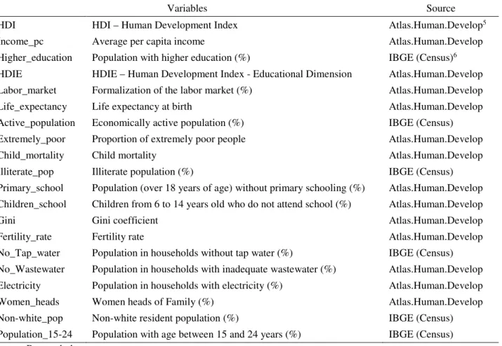
This paper covered the 5,565 municipalities in Brazil, specifically considering the year 2010. For the level of crime in the country, we use the rate of homicides per 100,000 inhabitants as a proxy, available in SIM – DATASUS (2015), following the literature on the subject matter. (SHIKIDA, 2009; SANTOS; SANTOS FILHO, 2011; UCHÔA; MENEZES, 2012; SHIKIDA; OLIVEIRA, 2012; PLASSA; PARRÉ, 2015). Although there is recent data for homicide rate in Brazil, we used 2010 alone for the present analysis due to the wide availability of variables related to municipal economic development for that year, from the Demographic Census and the Atlas of Human Development. In Table 1, we have the variables used to construct the EDI, along with their respective sources.
Table 1 – Variables used in the factor analysis model and their sources
Variables Source
HDI HDI – Human Development Index Atlas.Human.Develop5
Income_pc Average per capita income Atlas.Human.Develop
Higher_education Population with higher education (%) IBGE (Census)6
HDIE HDIE – Human Development Index - Educational Dimension Atlas.Human.Develop Labor_market Formalization of the labor market (%) Atlas.Human.Develop Life_expectancy Life expectancy at birth Atlas.Human.Develop Active_population Economically active population (%) IBGE (Census) Extremely_poor Proportion of extremely poor people Atlas.Human.Develop
Child_mortality Child mortality Atlas.Human.Develop
Illiterate_pop Illiterate population (%) IBGE (Census)
Primary_school Population (over 18 years of age) without primary schooling (%) Atlas.Human.Develop Children_school Children from 6 to 14 years old who do not attend school (%) Atlas.Human.Develop
Gini Gini coefficient Atlas.Human.Develop
Fertility_rate Fertility rate Atlas.Human.Develop
No_Tap_water Population in households without tap water (%) IBGE (Census) No_Wastewater Population in households with inadequate wastewater (%) Atlas.Human.Develop Electricity Population in households with electricity (%) Atlas.Human.Develop
Women_heads Women heads of Family (%) Atlas.Human.Develop
Non-white_pop Non-white resident population (%) IBGE (Census) Population_15-24 Population with age between 15 and 24 years (%) IBGE (Census) Source: Research data.
4. Spatial distribution of crime and its relations to economic development
The application of the factor analysis model for the twenty economic and social variables described in the previous section enabled the extraction of three factors with characteristic roots greater than one (O! ≥ 1). In addition, the Kaiser-Meyer-Olkin (KMO) test, which verifies the suitability of the sample for the factor analysis model, presented a value of 0.844, indicating that the set of variables have a sufficiently high correlation for the method used. Bartlett's sphericity test, in turn, was statistically significant7, rejecting the null hypothesis that the correlation matrix is equal to
5 Atlas of Human Development (2013). 6 Demographic Census (2010).
the identity matrix. Therefore, from the results of both tests, we can conclude that the sample is suitable for the factor analysis method.
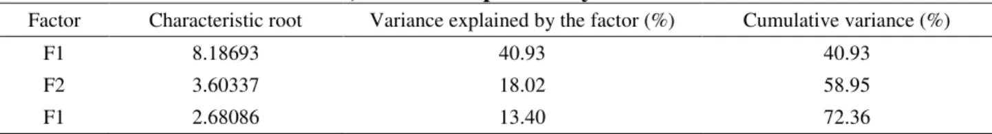
Table 2 brings the factors obtained, with their respective characteristic roots, as well as the explained and accumulated variance. The three factors were able to explain approximately 72.36% of the variance of the 20 variables selected. According to Hair et al. (2009), a cumulative variance greater than 60% is satisfactory, especially in the social sciences. In addition, the factor analysis method was able to summarize approximately 41% of the information contained in the 20 variables used in only one new variable (Factor 1). Therefore, the factors have been able to summarize the variables relatively well, deftly representing the socioeconomic development of Brazilian municipalities.
Table 2 – Characteristic root, variance explained by factor and accumulated variance
Factor Characteristic root Variance explained by the factor (%) Cumulative variance (%)
F1 8.18693 40.93 40.93
F2 3.60337 18.02 58.95
F1 2.68086 13.40 72.36
Source: Research data.
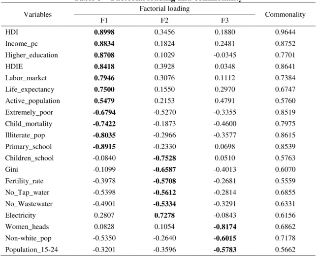
Finally, we performed the orthogonal rotation of the factors with the Varimax method. The results are in Table 3, which presents the factorial loadings of each factor, as well as the commonality of each variable. The results interpretation are: for each variable, it is considered which factor it contributes most, according to the absolute value of the factorial loadings (highlighted in bold).
It turns out that factor 1 is closely related to 11 of the 20 variables used, in addition to presenting a positive relationship with seven of them and negative with the remaining four. So, there are variables that contribute positively to the final value of Factor 1 as there are others that decrease it. Among the positives, we have: HDI, Income_pc, Higher_education, HDIE, Labor_makert, Life_expectancy, Active_population. Note that the variables are related to municipal socioeconomic development, with higher values representing a county that provides good material and social conditions for its population.
The negatively-related variables are: Extremely_poor, Child mortality, Primary_school. High values for the mentioned variables are related to localities with low socioeconomic development, justifying their the negative impact. Therefore, we named Factor 1, because it captures essentially socioeconomic characteristics, as the municipalities’ Socioeconomic Indicator.
Factor 2, in turn, is related to six of the 20 variables used in the factor analysis model, and only one has a positive impact. With respect to the negatives, we have: Children_school, Gini, Fertility rate; No_Tap_water, No_Wastewater. Lower values for the variables are related with socioeconomic underdevelopment due to the unwantedness of these characteristics. The only variable that contributes positively to Factor 2 is Electricity. Because it relates with infrastructure and social conditions, we named Factor 2 the Infrastructure and Social Indicator. As in the previous case, municipalities with a high value for this indicator present a higher level of development.
Finally, the last three variables used are negatively related to Factor 3, which are: Women_heads, women heads of Family (%); Non-white_pop, non-white resident population (%); Population_15-24, population with age between 15 and 24 years (%). Factor 3 relates mainly to population characteristics, thus, we called this factor the Population Characteristics Indicator.
After the estimation of factor scores for each Brazilian municipality, we built the Economic Development Index (EDI), as specified in the methodology. After its calculation, the index presented an average (;a) of 47.3 and standard deviation (oa) of 16.4. With these values, it was possible to define the economic development categories for the Brazilian municipalities, as in Table 4. Only 0.59% of Brazilian municipalities are part of the very high development category (VHD). On the opposite side, 1.37% of municipalities are in the very low development category (VLD),
which represents more than twice the number of VHD municipalities. In addition, more than half of the municipalities presented average development (HMD and HMD), which belong to the range from 30.9 to 63.8 (62.26%).
Table 3 – Factorial loading and commonality
Variables Factorial loading Commonality
F1 F2 F3 HDI 0.8998 0.3456 0.1880 0.9644 Income_pc 0.8834 0.1824 0.2481 0.8752 Higher_education 0.8708 0.1029 -0.0345 0.7701 HDIE 0.8418 0.3928 0.0348 0.8641 Labor_market 0.7946 0.3076 0.1112 0.7384 Life_expectancy 0.7500 0.1550 0.2970 0.6747 Active_population 0.5479 0.2153 0.4791 0.5760 Extremely_poor -0.6794 -0.5270 -0.3355 0.8519 Child_mortality -0.7422 -0.1873 -0.4600 0.7975 Illiterate_pop -0.8035 -0.2966 -0.3577 0.8615 Primary_school -0.8915 -0.2330 0.0698 0.8539 Children_school -0.0840 -0.7528 0.0510 0.5763 Gini -0.1099 -0.6587 -0.4013 0.6070 Fertility_rate -0.3978 -0.5708 -0.2681 0.5559 No_Tap_water -0.5398 -0.5612 -0.2814 0.6855 No_Wastewater -0.4901 -0.5334 -0.3291 0.6331 Electricity 0.2807 0.7278 -0.0843 0.6156 Women_heads 0.0828 0.1054 -0.8174 0.6862 Non-white_pop -0.5350 -0.2640 -0.6015 0.7178 Population_15-24 -0.3201 -0.3596 -0.5783 0.5662
Source: Research data.
Table 4 – Categories of the EDI
Categories Lower limit Upper Limit Municipalities Total Municipalities (%) VHD 80.2 100 33 0.59% HD 63.8 80.2 915 16.44% HMD 47.3 63.8 2073 37.25% LMD 30.9 47.3 1392 25.01% LD 14.4 30.9 1076 19.34% VLD 0 14.4 76 1.37%
Source: Research data.
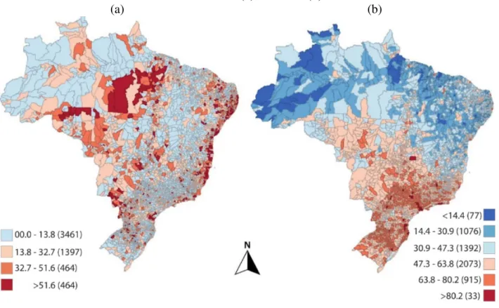
The main objective of this paper is to verify the relations between a given location’s crime rate and its level of economic development. Thus, Figure 1 shows the homicide rate spatial distribution throughout the Brazilian municipalities (a) (per 100,000 inhabitants), as well as for the Economic Development Index (EDI) (b) (distributed according to the categories identified).
Note that higher homicide rates (a) are essentially concentrated in three regions of the Brazilian territory: i) Coastal areas with large population concentration; ii) the Brazilian agricultural frontier,
located especially in Pará, Mato Grosso and Rondônia; iii) border regions with high flow of people in Paraná and Mato Grosso do Sul. Waiselfisz (2011), Andrade and Diniz (2013), Steeves et al. (2015) and Ceccato and Ceccato (2017) also identified the regions i), ii) and iii) with high crime rates. In addition, ii) and iii) are the main responsible, according to the authors, for the thesis of "Interiorization of crime" in the country. According to Santos and Santos Filho (2011), Steeves et al. (2015) and Ceccato and Ceccato (2017), this phenomenon occurs mainly due to the lower growth of homicide rates across the country's traditionally violent places, such as most state capitals and metropolitan regions, while interior regions have been showing rising rates of violent deaths.
Figure 1: Distribution of homicide rate and the EDI between Brazilian municipalities in 2010 – homicides (a) and EDI (b)
(a) (b)
Source: Research data.
Considering the EDI (b), we have a clear division of Brazil in two areas with different levels of development. The Central-South region of the country concentrates the majority of municipalities with high levels of economic development, with an EDI above the Brazilian average. On the other hand, in the North and Northeast, we have a concentration of underdeveloped municipalities, with most showing an EDI below the national average. These results are in line with those found by the Atlas of Human Development (2013), which identified the Central-South with most of the developed municipalities of the country while the underdeveloped ones predominate in the North and Northeast regions.
The spatial concentration of municipalities is visible for both variables analyzed (Figure 1). This is proven by Moran’s I coefficients (Table 5), whose values are positive and statistically significant at 1% regardless of the convention matrix applied. Thus, municipalities with high homicide rates or economic development tend to surround municipalities with high coefficients for the same variable (and vice versa). The spatial configuration is best captured with the three neighbors convention for both variables.
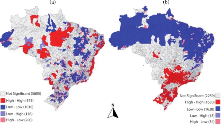
By using local spatial association indicators (LISA maps), we identified the existence of spatial clusters for crime rate (a) and the level of economic development (b) in Brazil. In both cases, the positive spatial concentration (high-high and low-low) maintained a similar configuration as in Figure 1, in which only the variables gross distribution was verified, without considering the
formation of significant spatial clusters. Therefore, the distribution in Figure 1, in fact, corresponds to the existence of spatial concentration for both variables.
Table 5 – Moran’s I for homicide rate and for the Economic development Index (EDI) - 2010
Weights matrix
Three neigh Five neigh Seven neigh Ten neigh
Homicide rate 0.29* 0.28* 0.27* 0.26*
Index – EDI 0.47* 0.45* 0.43* 0.42*
Note: * statistical significance of 1%.
Source: Research data.
Figure 2 – LISA for the homicide rate and the EDI between the Brazilian Municipalities in 2010 – homicides (a) and EDI (b)
(a) (b)
Source: Research data.
In addition, the spatial clusters identified for the homicide rate are apparently not located in the same regions as the clusters for the development level. The agricultural frontier region in the Amazon, for example, presents a large spatial concentration of homicides at the same time that it is a region with low economic development. For the state of Pará, for example, Chimeli and Soares (2017) found evidence that illegal logging is an important crime inductor in the state, while Adrande et al. (2013), Ceccato and Ceccato (2015) and Waiselfisz (2016) emphasize the role of land-use conflicts. The Brazilian coastline, especially in the Northeast, presents the same configuration, with high level of homicides (a) concomitantly to a Low-Low (or not significant) concentration for the EDI (b). In the opposite case, it is possible to cite some localities in the states of Minas Gerais, Rio Grande do Sul and Sao Paulo, where we have some Low-Low spatial clusters for crime (a) although they are regions with the highest level of development in the country.
Finally, we can mention some exceptions that do not follow the pattern identified previously: parts of the states of Rio de Janeiro and Espírito Santo, as well as the metropolitan Region of Curitiba (in the state of Paraná). Those regions present high economic development (b) while also
showing high crime rates (a). Coutollene et al. (2000) and Cerqueira (2010), for example, estimated that only in the city of Rio de Janeiro, the annual cost associated with crime reaches 5% of the city GDP. According to Waiselfisz (2016) and Ceccato and Ceccato (2017), the states of Rio de Janeiro and Espírito Santo have many “municipalities with predatory tourism”, which attract large amounts of temporary population especially in the summer, which can lead to an increase in their respective homicide rates. In addition, according to Santos (2009), Waiselfisz (2016) and Ceccato and Ceccato (2017), Brazilian states, especially RJ and ES, suffer from an inertial component in which regions with high crime tend to present similar values in later periods, characterizing them as “traditional” regions of violence. Finally, both phenomena help to understand the concentration of crime along the coastal regions of Brazil.
Regarding Curitiba, the results found are in line with Waiselfisz (2012), Andrade et al. (2013), Plassa and Parré (2015), Sass et al. (2016) and Anjos Junior et al. (2016), which identified in this metropolitan region the highest concentration of municipalities with high crime rate in the South. Anjos Junior et al. (2016) found that Paraná, and especially the Curitiba region, have a different dynamic when compared to other southern localities. In addition, the authors found that HDI, a development proxy, was not significant to explain the homicide rates in the area. Sass et al. (2016) identified that poverty and others socioeconomic conditions do not explain crime in the metropolitan region of Curitiba as expected, and that an increase in the police force is the best policy to reduce crime in the region.
However, these regions are set up as isolated cases when considering the entire Brazilian context. Analyzing maps (a) and (b) (Figure 2), the predominant configuration is that high development is associated with a lower crime rate (and vice versa). To test this hypothesis, we use some complementary methodologies, as the bivariate spatial autocorrelation and cluster analysis, seeking to better examine the relationship between the two variables.
In relation to the bivariate spatial autocorrelation, used with the intention of analyzing spatial dependence between different variables, we have a result of -0.10068, indicating a considerable
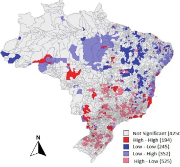
negative spatial association between crime and economic development. In other words, municipalities with low homicides have neighbors with high EDI (and vice versa), a hint that the hypothesis sustained in this paper can in fact be true. Plassa and Parré (2015) found similar results for the state of Paraná, adopting the same methodology. Figure 3, in turn, brings the results of bivariate local Moran’s I, which was calculated considering the EDI in relation to crime.
The Low-High (LH) and High-Low (HL) spatial clusters are those of higher interest in the present paper, because it seeks exactly an inverse relationship between the variables. The spatial associations with this configuration are 352 municipalities for LH and 525 for HL, i.e., 26.74% and 39.89% of the total respectively. Therefore, 26.74% of the country's municipalities are set up as low in development and high in crime rates, and they are concentrated in the Northeast and Northern regions of the country. On the other hand, 39.89% of municipalities have high development and low crime. They are located mainly in the Central-South region of Brazil.
In the next paragraphs, we present the results from cluster analysis, a multivariate statistics technique. In group analysis, the neighborhood relationship is not necessary – two municipalities may be located on opposite sides of the country and still belong to the same cluster. In addition, this multivariate technique groups information according to a given chosen criterion, and, in the end, there is no information left out, as the non-significant cases in spatial clusters. Therefore, we use cluster analysis as a complementary methodology. This procedure is a methodological contribution of this work, since there are no studies in the national literature that have used it to analyze crime and its relation to economic development.
Figure 3: Bivariate local Moran’s I between crime and the EDI for Brazilian municipalities in 2010
Source: Research data.
Figure 4 brings the homicide rate and development (EDI) Dendogram. Group analysis suggests that there are four clusters between the Brazilian municipalities that present similar characteristics between crime and the EDI. However, we have an unequal division between the clusters. Two groups (in the far right of the Dendogram) have a small amount of municipalities when compared to the other half (left).
Figure 4: Dendogram
Source: Research data.
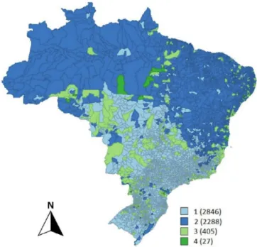
Figure 5 shows the cluster distribution, as well as the number of municipalities in each group. Remember that we used the Complete Linkage method, which classifies according to a criterion of dissimilarity. Therefore, it grouped municipalities with high economic development alongside low crime rate (and vice versa). The most part of Brazilian municipalities are grouped in two clusters. The largest is Cluster 1 with 2,846 municipalities (51.14% of the total), while Cluster 2 has 2,288 municipalities (41.11% of the total). Thus, by adding both clusters, we have approximately 92.25% of the total, representing the vast majority of Brazilian municipalities. Cluster 3, in turn, has 405
municipalities, while Cluster 4 has only 27, both representing 7.27% and 0.48% of the total, respectively. The low representativeness of Clusters 3 and, especially, 4, characterizes them as outliers, since they have certain elements that are not shared with the majority of Brazilian municipalities.
Figure 5: Cluster distribution of Brazilian municipalities in 2010
Source: Research data.
To better verify each cluster’s characteristics, Table 6 brings the homicide rate and Economic Development Index (EDI) averages for each group, as well as for Brazil. Cluster 1 presented an above-average value for the EDI and, at the same time, a below-average value for homicides. Cluster 2, in turn, presented a reverse dynamic, with low economic development and high crime rate, when comparted to the national levels. Thus, both corroborate the basic hypothesis raised by the present paper, that high crime rates are linked to municipalities with low economic development (and vice versa). Moreover, by representing about 92.25% of the country's municipalities, these two Clusters represent the majority of the Brazilian reality. Therefore, the relationship found by Shikida (2009), Shikida and Oliveira (2012) and Plassa and Parré (2015) between crime and economic development at regional levels proved to be true when expanded to all municipalities in the country.
Table 6 – Average homicide rate and economic development for the five clusters and for Brazil
Average Cluster 1 Cluster 2 Cluster 3 Cluster 4 Brazil9
Homicide 11.2 15.31 14.78 16.47 13.18
EDI 57.8 33.8 51.01 38.54 47.32
Source: Research data.
Cluster 4 presented the same features as Cluster 2, but with a slightly larger average for both variables. However, considering the Brazilian average, these Clusters’ municipalities are still “underdeveloped” and with high crime rates. In addition, Cluster 4 is not representative of the Brazilian reality (only 0.48% of municipalities) and its characteristics are different from the majority of municipalities. For example, in Figure 5, we have several municipalities from Cluster 3 that are located in the so-called Brazilian agricultural frontier in the Legal Amazon, in states such as
9 Average homicide rate (by 100,000 inhabitants) of Brazilian municipalities used by group analysis (Euclidean
Mato Grosso, Pará and Rondônia. According to Adrande and Diniz (2013), Waiselfisz (2016), Ceccato and Ceccato (2015) and Chimeli and Soares (2017), these regions presented rapid occupation and economic growth in recent decades, which caused many social conflicts related to natural resources and land use, and the crime-inhibiting institutions may not have accompanied this advancement.
Finally, Cluster 3 is the only one that actually contradicts the hypothesis that high development leads to lower crime rate. Even with the EDI average exceeding the national, the municipalities that integrate it still have high crime rates. This cluster corroborates the results found by the spatial clusters in Figure 3. Regions located in Rio de Janeiro, Espírito Santo and the metropolitan region of Curitiba maintained the same relationship, once again in line with the empirical evidences from Waiselfisz (2012), Andrade et al. (2013), Plassa and Parré (2015), Sass et al. (2016), Waiselfisz (2016) and Ceccato and Ceccato (2017).
However, cluster analysis, without considering the space, allowed the identification of some localities that also present this contradictory dynamics, especially in the states of Mato Grosso do Sul (MS) and Mato Grosso (MT). In addition, there is a concentration of municipalities of this cluster in border regions or that have suffered intense agricultural occupation in recent years, as the case of MS, MT and Goiás. The high crime concentration in those regions is also highlighted by Andrade et al. (2013), Waiselfisz (2016) and Ceccato and Ceccato (2017). According to Ceccato and Ceccato (2017, p. 227), border regions present this feature because they are “magnets for transnational organizations dealing with the smuggling of goods and/or weapons, piracy, and drug trafficking”.
Therefore, although the hypothesis is true for most Brazilian municipalities, there is a group, represented by Cluster 3, which deserves special attention on the part of researchers and public agents. In these localities, material and social well-being advancement will not necessarily lead to a decrease in crime rates due their idiosyncrasies. In addition, they are strategic localities for the country, because they are regions that have at least one of the following characteristics: i) high population density; ii) border regions subject to smuggling and trafficking of drugs and weapons; iii) regions with high economic dynamism. (WAISELFIZ, 2012; ANDRADE et al., 2013; PLASSA AND PARRÉ, 2015; SASS et al., 2016; WAISELFIZ, 2016; CECCATO; CECCATO, 2017). Therefore, these municipalities are extremely relevant for the Brazilian population, either directly or indirectly.
Hence, in order to identify the causes and consequences of this differentiated features, further investigations into these regions are necessary, and they can enable the construction of policies and actions that mitigate potential problems associated with crime.
5. Final considerations
The present paper sought to analyze the relationship between the homicide rate and economic development in the Brazilian municipalities. Firstly, we developed an Economic Development Index (EDI) with multivariate statistics techniques. The index was able to identify the existence of disparities throughout the Brazilian territory, especially a North-Northeast and Central-South dichotomy, with the latter concentrating most of the country’s developed municipalities. We also found positive spatial dependence on both crime and the EDI, as well as the existence of significant spatial clusters throughout the country. In other words, municipalities with high values for crime rate and/or economic development tend to have neighbors with similar features.
Regarding the relationship between crime and economic development, we found a significant bivariate spatial autocorrelation. However, unlike the previous case, the relationship was negative, with developed regions surrounded by low crime rate municipalities (and vice versa). This evidence sustains the basic hypothesis raised by this paper that there is an inverse relation between crime and economic development. Using cluster analysis, we also got evidence that supports the hypothesis that high economic development is a crime inhibitor for most Brazilian municipalities.
For the vast majority of them (those comprising Clusters 1, 2 and 4 - 92.73% of the total), the evidence supports that the best action against crime is the incentive to economic development.
However, there is a small number of municipalities, identified from spatial and cluster analyses, where economic development is not capable of barring crime advancement. Examples are the states of Rio de Janeiro and Espírito Santo, the metropolitan region of Curitiba, the agricultural frontier in the Legal Amazon and border regions. Since they present idiosyncrasies, these regions demand more investigations, especially considering their importance to Brazil and its population. Therefore, it is necessary that researchers and public agents take greater care of this issue in order to understand the reasons and consequences of their difference. With this in hands, the Brazilian society and government can undertake actions and public policies to reduce the crime growth in these regions, since economic development alone is not capable of doing it.
References
ALMEIDA, E. S. Econometria espacial aplicada. Campinas: Editora Alínea, 2012.
ALMEIDA, E. S.; HADDAD, E. A.; HEWINGS, G. J. The spatial pattern of crime in Minas Gerais: an exploratory analysis. Economia Aplicada, v. 9, n. 1, p. 39-55, 2005.
ALMEIDA, M. A. S. D.; GUANZIROLI, C. E. Análise exploratória espacial e convergência condicional das taxas de crimes em Minas Gerais nos anos 2000. In: Encontro Nacional de Economia, 41, 2013. Anais… Foz do Iguaçu: ANPEC, 2013.
ANDRESEN, M, A. Crime measures and the spatial analysis of criminal activity. British Journal of
Criminology, v. 46, n. 2, p. 258-285, 2005.
ANDRADE, L. T.; DINIZ, A. M. A. A reorganização espacial dos homicídios no Brasil e a tese da interiorização. Revista Brasileira de Estudos de População, v. 30, p. 171-191, 2013.
ANJOS JUNIOR, O. R.; CIRIACO, J. S.; BATISTA DA SILVA, M. V. Testando a hipótese de dependência espacial na taxa de crime dos municípios da região Sul do Brasil. In: Encontro de Economia da Região Sul, 19, 2016. Anais... Florianópolis: ANPEC, 2016.
ARAÚJO JR., A.; FAJNZYLBER, P. O que causa a criminalidade violenta no Brasil? Uma
análise a partir do modelo econômico do crime: 1981 a 1996. Centro de Desenvolvimento e
Planejamento Regional, Universidade Federal de Minas Gerais. Belo Horizonte, 2001. (Texto de Discussão, n. 162).
ATLAS OF HUMAN DEVELOPMENT, 2013. Disponível em: <http://atlasbrasil.org.br/2013/>. Acesso em: 30 março de 2018.
BARCELLOS, C.; ZALUAR, A. Homicídios e disputas territoriais nas favelas do Rio de Janeiro.
Revista de Saúde Pública, v. 48, n. 1, p. 94-102, 2014.
BEATO FILHO, C. C; ASSUNÇÃO, R. M; SILVA, B. F. A; MARINHO, F. C; REIS, I. A; ALMEIDA, M. C. M. Conglomerados de homicídios e o tráfico de drogas em Belo Horizonte, Minas Gerais, Brasil, de 1995 a 1999. Cadernos de Saúde Pública, v. 17, n. 5, p. 1163-1171, 2001.
BECKER, G. S. Crime and punishment: an economic approach. Journal of Political Economy, v. 76, n. 2, p. 169-217, 1968.
BECKER, K. L.; KASSOUF, A. L. Uma análise do efeito dos gastos públicos em educação sobre a criminalidade no Brasil. Economia e Sociedade, v. 26, n. 1, p. 215-242, 2017.
BRASIL. Secretaria da Presidência da República. Custos econômicos da criminalidade no Brasil. Relatório de conjuntura nº 4. Brasília, 2018.
BRITO, F. O deslocamento da população brasileira para as metrópoles. Estudos Avançados, v. 20, n. 57, p. 221-236, 2006.
BURSIK, R. J. Social disorganizations: problems and prospects. Criminology, n. 26, p. 519-551, 1988.
CANO, I. Análise espacial da violência no município do Rio de Janeiro. In: NAJAR, A. L.; MARQUES, E. C. (org.). Saúde e espaço: estudos metodológicos e técnicas de análise. Rio de Janeiro: Fiocruz, 1998, p. 239-274.
CANO, I.; BORGES, D. Homicídios na Adolescência no Brasil: IHA 2009-2010. Rio de Janeiro: Observatório de Favelas, 2012.
CASTRO, L. S; LIMA, J. E. A soja e o estado do Mato Grosso: existe alguma relação entre o plantio da cultura e o desenvolvimento dos municípios? Revista Brasileira de Estudos
Regionais e Urbanos, v. 10, n. 2, p. 177-198, 2016.
CECCATO, V.; CECCATO, H. Violence in the rural global south: trends, patterns, and tales from the Brazilian countryside. Criminal Justice Review, v. 42, n. 3, p. 270–290, 2017.
CERQUEIRA, D.C. Causas e consequências do crime no Brasil. Tese (Doutorado em Economia) – Departamento de Economia, Pontificada Universidade Católica do Rio de Janeiro. Rio de Janeiro, 2010.
CHIMELI, A. B; SOARES, R. R. The use of violence in illegal markets: evidence from Mahogany trade in the Brazilian Amazon. American Economic Journal: Applied Economics, v. 9, n. 4, p. 30-57, 2017.
CRUZ, O. G.; CARVALHO, M. S. Mortalidade por causas externas: análise exploratória espacial, Região Sudeste/Brasil. In: Encontro Nacional de Estudos Populacionais, 11, 1998. Rio de Janeiro: ABEP, 1998.
DATASUS. Sistema Único de Saúde do Brasil, Secretaria de Gestão Estratégica e Participativa, Ministério da Saúde, 2015. Disponível em: <http://datasus.saude.gov.br/>. Acesso em: 25 de março 2018.
FALLAHI, F.; POURTAGHI, H.; RODRÍGUEZ, G. The unemployment rate, unemployment volatility, and crime. International Journal of Social Economics, v. 39, n. 6, p. 440-448, 2012. GLAESER, E. L. SACERDOTE, B. Why is there crime in cities? Journal of Political Economy, v.
107, n.6, p. 225-258, 1999.
HAIR, J. F.; ANDERSON, R. E.; TATHAM, R. L.; BLACK, W. C. Análise multivariada de dados. 6 ed. New Jersey: Prentice Hall, 2009.
KAISER, H. F. The varimax criterion for analytic rotation in factor analysis. Psychometrika, v. 23, n. 1, p. 187-200, 1958.
KUBRIN, C. E. Social disorganization theory: then, now, and in the future. In: KROHN, D. M.; LIZOTTE, J. A.; HALL, P. G. (ed.). Handbook on crime and deviance. New York, NY: Springer New York, p. 225-236, 2009.
KUME, L. Uma estimativa dos determinantes da taxa de criminalidade brasileira: uma aplicação em painel dinâmico. In: Encontro Nacional de Economia, 32, 2004. Anais... João Pessoa: ANEPC, 2004.
LOUREIRO, A. O. F.; CARVALHO JR., J. R. A. O impacto dos gastos públicos sobre a criminalidade no Brasil. In: Encontro Nacional de Economia, 35, 2007. Anais... Recife: ANPEC, 2007.
MELO, C. O.; PARRÉ J. L. Índice de desenvolvimento rural dos municípios paranaenses: determinantes e hierarquização. Brasília. Revista de Economia e Sociologia Rural, v. 45, n. 2, p. 329-365, 2007.
MENDONÇA, M. J. C; LOUREIRO, P. R. A; SACHIDA, A. Criminalidade e desigualdade social
no Brasil. Rio de Janeiro: IPEA, 2003. (Texto para Discussão, n. 967).
MINGOTI, S. A. Análise de dados através de métodos de estatística multivariada: uma abordagem aplicada. Belo Horizonte: UFMG, 2005.
MONSANO, F. H; PARRÉ, J. L.; PEREIRA, M. F. Análise fatorial aplicada para a classificação das incubadoras das empresas de base tecnológica do Paraná. Revista Brasileira de Estudos
Regionais e Urbanos, v. 11, n. 2, p. 133-151, 2017.
OLIVEIRA, C. Análise espacial da criminalidade no Rio Grande do Sul. Revista de Economia, v. 34, n. 3, p. 35-60, 2008.
PAIM, J. S.; COSTA, M. C. N.; MASCARENHAS, J. C. S.; SILVA, L. M. V. Distribuição espacial da violência: mortalidade por causas externas em Salvador. Revista Panamericana de Saúde
Pública, v. 6, p. 321-332, 1999.
PLASSA, W.; PARRÉ, J. L. A Violência no estado do Paraná: uma análise espacial das taxas de homicídios e de fatores socioeconômicos. In: Encontro Nacional da Associação Brasileira de Estudos Regionais e Urbano. Anais… Curitiba: ABER, 2015.
PHILLIPS, J.; LAND, K. The link between unemployment and crime rate fluctuations: an analysis at the county, state, and national levels. Social Science Research, v. 41, n. 3, p. 681-694, 2012. RESENDE, J. P; ANDRADE, M. V. Crime social, castigo social: desigualdade de renda e taxas de
criminalidade nos grandes municípios brasileiros. Estudos Econômicos, v. 41, n. 1, p. 173-195, 2011.
RIVERO, P. S. Segregação urbana e distribuição da violência: homicídios georreferenciados no município do Rio de Janeiro. Revista de Estudos de Conflito e Controle Social, v. 9, n.3, p. 117-142, 2010.
SANTOS, M. J. Dinâmica temporal da criminalidade: mais evidências sobre o “efeito inércia” nas taxas de crimes letais nos estados brasileiros. EconomiA, v. 10, n. 1, p. 169-194, 2009.
SANTOS, M. J.; SANTOS FILHO, J. I. Convergência das taxas de crimes no território brasileiro.
EconomiA, v. 12, n. 1, p. 131-147, 2011.
SACHSIDA, A.; MENDONÇA, M. J. C.; LOUREIRO, P. R. A; GUTIERREZ, M. B. S. Inequality and criminality revisited: further evidence from Brazil. Empirical Economics, v. 39, n. 1, p. 93-109, 2010.
SASS, K. S; PORSSE, A. A.; SILVA, E. R. H. Determinantes das taxas de crimes no Paraná: uma abordagem espacial. Revista Brasileira de Estudos Regionais e Urbanos, v. 10, n. 1, p. 44-63, 2016.
SCORZAFAVE, L; SOARES, M. K. Income Inequality and Pecuniary crimes. Economics Letters, v. 104, pp. 40-42, 2009.
SEN, A. Desenvolvimento como liberdade. São Paulo: Companhia das Letras, 2000. SHAW, C. R.; MCKAY, H. D. Juvenile delinquency and urban areas. Chicago: Ill, 1942.
SHIKIDA, P. F. A. Crimes violentos e desenvolvimento socioeconômico: um estudo para o Estado do Paraná. Direitos Fundamentais & Justiça, v. 2, n. 5, p. 144-161, 2009.
SHIKIDA, P. F. A.; OLIVEIRA, H. V. N. Crimes violentos e desenvolvimento socioeconômico: um estudo sobre a mesorregião Oeste do Paraná. Revista Brasileira de Gestão e
Desenvolvimento Regional, v. 8, n. 3, p. 99-114, 2012.
STEEVES, G. M.; PETTERINI, F. C.; MOURA, G. V. The interiorization of Brazilian violence, policing, and economic growth. EconomiA, v. 16, n. 3, p. 359-375, 2015.
STEGE, A. L.; PARRÉ, J. L. Fatores que determinam o desenvolvimento rural nas microrregiões do Brasil. Confins, n. 19, p. 18-32, 2013.
SULIANO, D. C.; OLIVEIRA, J. L. Avaliação do programa Ronda do Quarteirão na Região Metropolitana de Fortaleza (Ceará). Revista Brasileira de Estudos Regionais e Urbanos, v. 7, n. 2, p. 52-67, 2013.
SZWARCWALD, C. L; CASTILHO, E. A. Mortalidade por armas de fogo no estado do Rio de Janeiro, Brasil: uma análise espacial, Revista Panamericana de Saúde Pública, v. 3, n. 4, p. 161-170, 1998.
UCHOA, C. F. MENEZES, T. A. D; Spillover espacial da criminalidade: uma aplicação de painel espacial, para os estados Brasileiros. In: Encontro Nacional de Economia, 40, 2012. Porto de Galinhas: ANPEC, 2012.
WAISELFISZ, J. J. Mapa da violência 2012: os novos padrões da violência homicida no Brasil. São Paulo: Instituto Sangari, 2011.
WAISELFISZ, J. J. Mapa da violência 2016: homicídios por armas de fogo. São Paulo: Instituto Sangari, 2016.
WHO. World Health Organization. Global Health Observatory data repository. Homicide Estimates
by country. Disponível em:
<http://apps.who.int/gho/data/view.main.VIOLENCE-HOMICIDE>. Acesso em: 25 janeiro de 2019.
ORCID
Pedro Henrique Batista de Barros https://orcid.org/0000-0002-7968-0197 Isadora Salvalaggio Baggio https://orcid.org/0000-0003-2348-8662 Alysson Luiz Stege https://orcid.org/0000-0001-9266-1890
Cleise Maria de Almeida Tupich Hilgemberg https://orcid.org/0000-0002-4743-0089