CINTAL - Centro de Investiga¸
c˜
ao Tecnol´
ogica do Algarve
Universidade do Algarve
Tomografia Passiva Costiera
(TOMPACO)
Data Report - Phase 1
S´
ergio M.M. Jesus
Rep 01/01 - SiPLAB
15/Mar/2001
University of Algarve tel: +351-289800131 Campus da Penha fax: +351-289864258
Work requested by
CINTAL
Universidade do Algarve, Campus da Penha,
8000 Faro, Portugal
tel: +351-289800131, [email protected], www.ualg.pt/cintal
Laboratory performing
SiPLAB - Signal Processing Laboratory
the work
Universidade do Algarve, FCT, Campus de Gambelas,
8000 Faro, Portugal
tel: +351-289800949, [email protected],
www.ualg.pt/uceh/adeec/siplab
Project
TOMPACO - CNR, Italy
Title
TOMografia PAssiva COstiera - Data Report (Phase 1)
Author
S´
ergio M.M. Jesus
Date
March 15, 2001
Reference
01/01 - SiPLAB
Number of pages
40 (forty)
Abstract
This report describes the data acquired during the
INTIFANTE’00 sea trial that took place from 9 - 29 October
2000, off the Tr´
oia Peninsula, near Set´
ubal, Portugal.
Clearance level
UNCLASSIFIED
Distribution list
DUNE (1), ENEA (1), IH (1), IST (1), SACLANTCEN (1),
SiPLAB (1), CINTAL (2)
Total number of copies
8 (eight)
Foreword and Acknowledgment
This report presents all the real data relevant to the TOMPACO project acquired during the IN-TIFANTE’00 sea trial, as a specific request to fullfill the requirements for completation of phase 1 of the CINTAL - DUNE contract. The INTIFANTE’00 sea trial took place off the Tr´oia Peninsula, near Set´ubal, approximately 50 km south of Lisbon, Portugal, during the period 9 - 29 October 2000.
The institutions responsible for the sea trial are:
• Instituto Hidrogr´afico, Rua das Trinas 49, Lisboa, Portugal. • CINTAL, Universidade do Algarve, Faro, Portugal.
• ISR, Instituto Superior T´ecnico, Lisboa, Portugal.
Other institutions involved are:
• Ente Nazionale per l’Energia ed l’Ambiente, La Spezia, It´alia
The INTIFANTE organizers would like to thank: • the crew of the research vessel NRP D. Carlos I
• the NATO SACLANT Undersea Research Centre for lending the acoustic sound source and power amplifier.
• Enrico Muzi, from SACLANTCEN, for his participation in the acoustic source preparation and testing.
Contents
1 Introduction 7
2 The INTIFANTE’00 sea trial 9
2.1 Generalities and sea trial area . . . 9
2.2 List and description of Events . . . 11
3 Environmental data 12 3.1 Bottom properties and bathymetry . . . 12
3.1.1 Site bathymetry . . . 12 3.1.2 Sediment characteristics . . . 13 3.2 Hydrological data . . . 13 3.2.1 XBT data . . . 13 3.2.2 Thermistor data . . . 15 4 Experiment geometry 18 4.1 Ship position . . . 18
4.1.1 Event 4: in shore range-dependent track . . . 18
4.1.2 Event 5: out shore range-dependent track . . . 19
4.1.3 Event 6: arc-shaped track . . . 19
4.2 Source depth . . . 20
4.3 Receiver depth and tilt . . . 22
5 Acoustic data 25 5.1 Transmitted signals . . . 25
5.2 Received signals . . . 25
5.3 High-pass hydrophone filtering . . . 26
5.4 Event 4: range-dependent acoustic transmissions . . . 27
5.5 Event 5: pseudorandom noise transmissions . . . 29
5.6 Event 6: self-noise generated transmissions . . . 30
6 Conclusion 38
A INTIFANTE’00 CD-ROM list 39
1
Introduction
Ocean Acoustic Tomography (OAT) is now a well established technique for remote large scale ocean monitoring [1],[2]. The main objective of ocean monitoring studies is to discriminate small variations in the mean ocean temperature over a given period of time. To that end, integration over large ocean distances plays an important role. At smaller scale, say, in coastal waters, tomography aims at the online detection of temperature evolution in space and time. In that case, the range integration effect provided by OAT is a drawback and prEvents fine scale observation of fronts, internal waves, etc... Thus, at smaller scales, the need for higher spatial discrimination is to be achieved through a denser acoustic griding. Dense acoustic griding means multiple source-receiver pairs over a given area at a given time. This is expensive and in many cases unfeasible with common techniques of controlled source-receiver pairs, in which the acoustic signal emitted by the source and the source-receiver geometry have to be known at all times during the tomography observations.
The TOMPACO project1 aims at developing and testing ocean tomography techniques for
ob-taining a dense space-time acoustic griding at low cost, by relaxing the control on the source signal and geometry. In practice this means using alternative acoustic sources readily available in the ocean such as, for example, the noise radiated by ships of opportunity close or crossing the area of interest. Making a parallel with the sonar nomenclature, classic OAT will be termed as active tomography, while under the no-source-control concept the term passive tomography is introduced. The concept of using ships of opportunity as tomography sources is particularly appealing for coastal applications where they abbound in places like nearby busy ports, merchant shipping routes, ferry lines, fishing areas, etc... The main challenge faced by passsive tomography, and therefore by TOMPACO, is to account for the unpredictibility of the sound source in the tomographic procedure. That unpre-dictibility relates both to the source emitted signal and to the source-receiver geometry. The study of the impact of these two factors in the acoustic tomographic inversion process is the main goal of the TOMPACO project.
The INTIFANTE’00 sea trial2 was carried out in the vicinity of Set´ubal, situated approximately
50 km to the south of Lisbon, in Portugal, during the period from 9 to 29 October, 2000. The leading institutions were the Instituto Hidrogr´afico that carried out the oceanographic observations and managed the research vessel NRP D. Carlos I, CINTAL/UALG that provided the acoustic data acquisition system and the emitted source signal control and IST that was in charge of the high frequency data communications testing. Other collaborating/participating institutions were the NATO SACLANT Undersea Research Centre with the loan of the acoustic sound source and respective power amplifier and the Ente Nazionale per l’Energia e l’Ambiente (ENEA) that partic-ipated in the hydrological survey.
This sea trial served a number of specific purposes under the leading projects INTIMATE and INFANTE, but one day was reserved to acquire acoustic data to test the passive tomography concept under the TOMPACO project. The experiment area was a rectangular box situated in the border of the continental platform with depths varying from 60 to 140 m and including a sharp submarine canyon (the Set´ubal canyon) with depths reaching over 500 m. As an overview of the thecnical aspects involved in the experiment, it can be referred that acoustic signals were transmitted with an acoustic projector from onboard NRP D. Carlos I and received on a moored 16 hydrophone-4m spacing Vertical Line Array (VLA). The acoustic aperture of the vertical array was located between
1TOMPACO stands for ”TOMografia PAssiva COstiera” (Passive Coastal Tomography), a
project finnanced by the Consiglio Nazionale della Ricerca (CNR), Italy.
2INTIFANTE is a madeup acronym from INTImate and inFANTE, the two projects leading the
30 and 90 m in a 120 m water column. The acoustic signals received in the VLA were transmitted via an RF link to the research ship NRP D. Carlos I, processed, monitored and stored. Various signals were emitted by the sound projector ranging from linear frequency modulated (LFM) 2 second long upsweeps, to broadband computer generated white noise. Recordings were also made with the NRP D. Carlos I acting as source signal for the passive tomography testing purpose.
This report is organized as follows: section 2 gives an overview of the INTIFANTE’00 sea trial. Section 3 deals with the description of the environmental data, such as bathymetry, bottom prop-erties and hydrological information. Section 4 describes the overall geometry of the experiment like ship’s position and source - receiver geometry and finally section 5 describes the acoustic data gathered at the VLA. Some conclusions are drawn in section 6.
2
The INTIFANTE’00 sea trial
2.1
Generalities and sea trial area
The INTIFANTE’00 experiment was carried out in the period from 9 - 29 October 2000, off the town of Set´ubal, 50 km south from Lisbon, Portugal. The research vessel NRP D. Carlos I, managed by IH, was in charge of deploying all equipment, sending and receiving all signals to/from vertical array and making the necessary environmental surveys. The experimental scenario is depicted in the drawing of figure 2.1.
∼110 m
Real Data Acquisition Scenario
INTIMATE'00, OUT 2000 - SW Setubal site
Sediment Setubal Canyon ∼500 m Setubal 38º30’ 9º00’ 8º45’ 38º15’ NRP Dom Carlos UltraLight Vertical Array (ULVA) SoundSource
‘
‘
Figure 2.1: INTIFANTE’00 experimental scenario
The acoustic receiver was a 16-hydrophone 4-m spacing VLA suspended from the sea surface by a free floating rubber hose for wave action decoupling (see figure 2.2). The array also had a number of non-acoustic sensors like 8 thermistors, 2 tiltmeters and 2 pressure gauges. All signals received at the array were sampled and multiplexed in a telemetry unit, cabled to the surface buoy to be transmitted via an high speed data link to the NRP D. Carlos I. On board ship, the signals were demultiplexed, monitored and saved to disk together with GPS time synchronization marks allowing for absolute time datation. The NRP D. Carlos I was also transmitting acoustic signals with a sound projector imerged at variable depth depending whether on station or under tow. Emitted signals were computer generated and then transmitted to the power amplifier at specified times synchronous with GPS, and therefore also synchronous to the received signal datation scheme.
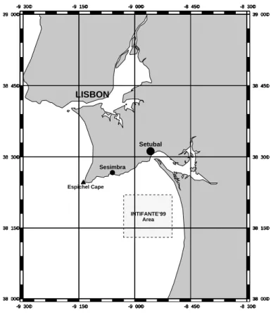
Ship movements were performed within a specified experiment sea trial area. The bounding box reserved for the sea trial is shown in figure 2.3 with coordinates:
Figure 2.2: Vertical line array structure.
Table 1: Experimental site bounding box
9◦ 3’ 0” W, 38◦ 22’ 0” N 8◦ 50’ 0” W, 38◦ 22’ 0” N 9◦ 3’ 0” W, 38◦ 13’ 0” N 8◦ 50’ 0” W, 38◦ 13’ 0” N
The choice of this area was made based on a number of factors among which that it is naturally protected from North winds by the Espichel Cape (North - West from site) and guarantees stable conditions for the development of work at sea. This is a relatively well known area from the oceanographic, hydrological and geophysical points of view as it has been previously explored by IH. The area itself is a portion of the continental platform with various bathymetric characteristics as shown in the detailed figure 2.4. The area is extending to shore in its eastern side attaining depths as low as 40 m, to northwest in a relatively range independent plateau at a 120 m depth, to the southwest nearly at the shelf edge at 200 m depth. The area is crossed from west to east by the Set´ubal Canyon that reaches depths as low as 800 m and extending into the continental plateau for about 20 miles. As can be seen in the sediment structure shown in figure 2.4, the bottom of the area is predominantely covered by sand and mud with a few localized rock patches. The bottom type is largely invariant in the plateau zone and the Canyon, while strongly variant when approaching shore.
The three black lines in figure 2.4 represent the acoustic transmission legs, while the crossing point is the VLA location; T2, T4 and T5 denote the locations of the currentmeter line moorings used during this sea trial. Figure 2.4 depicts the experimental area and sea trial geometry as planned prior to the experiment itself. Actual mooring locations and ship movements are given in the next chapters.
-9˚ 30' -9˚ 30' -9˚ 15' -9˚ 15' -9˚ 00' -9˚ 00' -8˚ 45' -8˚ 45' -8˚ 30' -8˚ 30' 38˚ 00' 38˚ 00' 38˚ 15' 38˚ 15' 38˚ 30' 38˚ 30' 38˚ 45' 38˚ 45' 39˚ 00' 39˚ 00' -9˚ 30' -9˚ 30' -9˚ 15' -9˚ 15' -9˚ 00' -9˚ 00' -8˚ 45' -8˚ 45' -8˚ 30' -8˚ 30' 38˚ 00' 38˚ 00' 38˚ 15' 38˚ 15' 38˚ 30' 38˚ 30' 38˚ 45' 38˚ 45' 39˚ 00' 39˚ 00' -9˚ 30' -9˚ 30' -9˚ 15' -9˚ 15' -9˚ 00' -9˚ 00' -8˚ 45' -8˚ 45' -8˚ 30' -8˚ 30' 38˚ 00' 38˚ 00' 38˚ 15' 38˚ 15' 38˚ 30' 38˚ 30' 38˚ 45' 38˚ 45' 39˚ 00' 39˚ 00' -9˚ 30' -9˚ 30' -9˚ 15' -9˚ 15' -9˚ 00' -9˚ 00' -8˚ 45' -8˚ 45' -8˚ 30' -8˚ 30' 38˚ 00' 38˚ 00' 38˚ 15' 38˚ 15' 38˚ 30' 38˚ 30' 38˚ 45' 38˚ 45' 39˚ 00' 39˚ 00' -9˚ 30' -9˚ 30' -9˚ 15' -9˚ 15' -9˚ 00' -9˚ 00' -8˚ 45' -8˚ 45' -8˚ 30' -8˚ 30' 38˚ 00' 38˚ 00' 38˚ 15' 38˚ 15' 38˚ 30' 38˚ 30' 38˚ 45' 38˚ 45' 39˚ 00' 39˚ 00' INTIFANTE’99 Area LISBON Sesimbra Setubal Espichel Cape
Figure 2.3: Localization of the experimental site
2.2
List and description of Events
The full list of Events planned for the INTIFANTE’00 sea trial is detailed in the Test Plan [3]. The Events of concern for TOMPACO are numbers 4, 5 and6 conducted during days 17-18 October as referred to in table 2.
Table 2: TOMPACO Event list
Event Start End Signal Description date-time(UTC) date-time(UTC)
Ev4 17/10-17:22 17/10-21:43 A3 transmitted LFM sweeps Ev5 17/10-22:20 18/10-01:00 C2 random signal
Ev6 18/10-02:20 18/10-03:20 ship ship noise
Events 4,5 and 6 were differentiated by the type of signals being transmitted . The three Events listed in table 2 were performed along the northeast transmission leg or nearby the VA so we will concentrate in that area in the sequel.
(1)Sand, (2)Mud, (3)Sand and gravel, (4)Rock.
Figure 2.4: Bathymetry and bottom structure
3
Environmental data
This section deals with the description of all non-acoustic site specific information gathered during the sea trial like bathymetry, bottom properties and water column temperature measurements.
3.1
Bottom properties and bathymetry
3.1.1
Site bathymetry
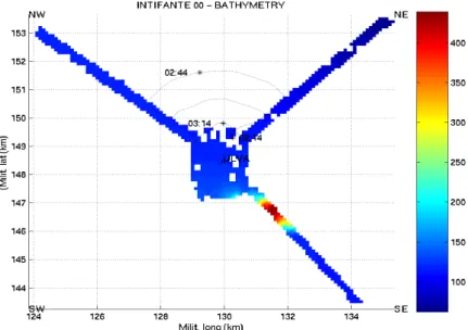
The sea trial area bathymetry was extensively surveyed by NRP D. Carlos I during the week 23 -29 October. A partial bathimetry map along the acoustic transmission tracks is given in figure 3.1. The full survey will be available in the IH report.
Figure 3.1: Site bathymetry along the acoustic transmission tracks (depth in m). VLA
location is denoted by ?.
3.1.2
Sediment characteristics
The acoustic transmission tracks have been surveyed during the INTIFANTE’99 with both a sidescan sonar and a light seismic Sparker system. During INTIFANTE’00 a second sidescan sonar survey was performed in the last sea trial week and will be included in the IH report.
3.2
Hydrological data
Hydrological data encompasses XBT and thermistor recordings. XBT casts were performed by ENEA from onboard D. Carlos I at various times. Thermistor recordings were made at the VLA location by the built in sensors.
3.2.1
XBT data
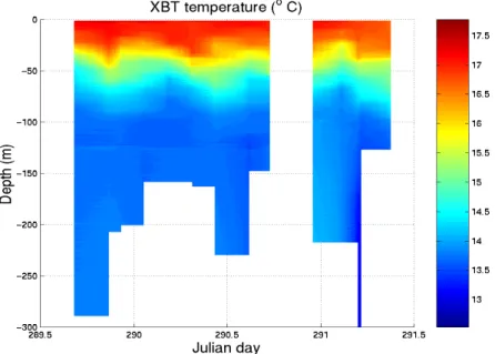
XBT casts were made approximately every 3 hours with the objective of capturing the tidal evolu-tion. Figure 3.2 shows 14 XBT recordings in (a) and the respective calculated sound velocity profiles (b). The displacement that can be seen in the first 4 calculated sound velocity profiles is due to an erroneous salinity setting during the cast itself. A strong downward refracting gradient can be seen
at an approximate depth of 10 m to over 50 m. The oscillation of the termocline along time can be seen in figure 3.3, where, even if largely undersampled, a semi-diurnal tidal effect can be clearly seen.
Figure 3.2: XBT data: temperature (a) and calculted sound velocity (b).
Figure 3.3: Recorded XBT temperature variation through time.
From a spatial point of view XBT casts were made from NRP D. Carlos and therefore always at the source location while the ship was moving along the various tracks performing acoustic transmissions. Figure 3.4 shows the positions of all XBT’s in the sea trial area together with the track fast bathymetry and the VLA position.
Figure 3.4: Location of XBT casts denoted by the
× positions.
3.2.2
Thermistor data
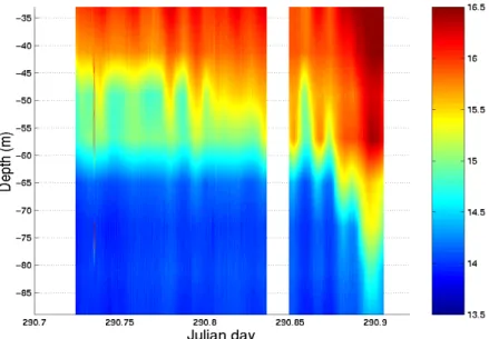
Temperature data was gathered from the thermistor sensors colocated with the VLA. While the XBT casts were supposed to capture the semi-diurnal behaviour of the tidal flux and a high-resolution spatial variation of the temperature field in the water column, the thermistor sensors were intended to obtain a high temporal resolution at selected depths and at fixed locations. The VLA has 8 temperature sensors with a 8 m spacing. The first sensor is located 3 m below the shallowest pressure gauge that was recording a mean depth of 30 m. So, temperature was recorded at approximate depths of 33, 41, 49, 57, 65, 73, 81 and 89 m, depending on the precision of the pressure gauge sensor and tilt of the vertical array.
The temperature field is shown in figures 3.5 to 3.7 for Events 4, 5 and 6 respectively. Event 4 lasted for approximately 4 hours and 20 minutes with a 20 minute interruption. Event 5 lasted for approximately 2.5 hours and Event 6 for approximately 1 hour. During that period the evolution of the water column temperature is highly consistent with small scale perturbations of the thermocline below 30 m depth (see figure 3.3).
Figure 3.5: Temperature field recorded at the VLA during Event 4.
4
Experiment geometry
This section describes the ship’s position as logged from GPS during the experiment. The relative position between source and receiver is deduced from the known VLA mooring position and the ship GPS log. The position of the VLA elements is estimated from the depth sensor and tilt recordings. Source depth is deduced from the source colocated depth sensor recordings and cable scope.
4.1
Ship position
Ship position was permanently recorded through the onboard GPS navigation system and by a parallel GPS system connected to the data recording station. In order to avoid confusion between several parallel tracks from different systems only the data provided by the data recording station GPS is used. Figures 4.1 to 4.6 show all the ship’s positioning data for Events 4,5 and 6.
4.1.1
Event 4: in shore range-dependent track
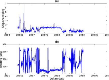
During Event 4, NRP D. Carlos I was supposed to start transmissions close by the VLA and then steam to location C along the NE leg. Arriving at location C she should keep the station for 1 hour. The GPS data is shown in figures 4.1 for ship’s speed (a) and heading (b) and in figure 4.2 for ship’s course along time.
Figure 4.1: Event 4: ship speed (a) and ship’s heading (b).
During the first part of the Event, and acording to figure 4.2, the ship was drifting by the VLA. After aproximately time 290.74, the ship took course by 50 degrees, which roughly corresponds to the orientation of leg C, at an approximate constant speed of 1 kn. After 290.81, the ship reached point
C and then drifted SE during the remaining time of the Event with an interruption of approximately 20 minutes for changing the transmitted code signal (see figure 4.2).
Figure 4.2: Ship course during Event 4.
4.1.2
Event 5: out shore range-dependent track
This Event started with the ship at location C and then steaming to the VLA along the NE leg. The GPS data is shown in figures 4.3 for ship’s speed (a) and heading (b) and in figure 4.4 for ship’s course along time. As planned the ship was held nearly at position C in the NE leg, during half hour at very slow speed and with a highly variable heading and then took a steady course towards the VLA at approximately 2 kn. At about 00:00, NRP D. Carlos I cercled the VLA at a 750 m radius from NE to NW. Event 5 ended at 00:47.
4.1.3
Event 6: arc-shaped track
During Event 6 it was planned doe the ship to perform a constant range track from the VLA location on the Northern sector between the NW and NE legs. This track is shown in figure 4.6 starting along the NE leg and performing first the 3 km range radius and then the 1.5 km radius. This path was followed at a high speed of approximately 10 kn as it can be seen in plot (a) of figure 4.5 with, however a few slowdowns during ship turns. Ship’s heading was monotonically changing along the arc cercle path as seen in plot (b) of the same figure.
Figure 4.3: Event 5: ship speed (a) and ship’s heading (b).
Figure 4.4: Ship course during Event 5.
4.2
Source depth
The pressure gauge inserted in the acoustic source failed to work due to a driving cable malfunction during the testing phase. An alternative self-recording pressure gauge was attached to the acoustic source tow cable at approximatelly 1.5 m from the source. The tow cable was tickmarked every 5 m.
Figure 4.5: Event 6: ship speed (a) and ship’s heading (b).
Figure 4.6: Ship course during Event 6.
After a given moment that depth sensor was also broken. From that moment on we are reduced to work with the paycable vs. depth calibration figures given by SACLANTCEN for that source and tow cable reproduced in figure 4.7. Source cable scope during the three Events is shown in table 3.
Table 3: Acoustic source cable scope.
Event Start End Cable scope date-time(UTC) date-time(UTC) (m) Ev4 17/10-17:22 17/10-21:43 47 Ev5 17/10-22:20 18/10-01:00 47 Ev6 18/10-02:20 18/10-03:20
-Figure 4.7: HX90 source depth as a function of cable length for various ship speeds.
4.3
Receiver depth and tilt
The vertical line array was equiped with two pressure gauges and two X-Y tiltmeters. The recordings of depth and tilt sensors are shown in figures 4.8 to 4.10 for Events 4, 5 and 6 respectively. During Event 4 both the shallowest and deepest depth sensors are relatively stable through time around 30.5 and 92.5 m depth respectively(4.8(a) and (b)). The distance of 62 m between them is consistent with the physical length of the array, denoting however a possible small array tilt. Plots (c) and (d) of figure 4.8, relative to the tilt sensors, are much more difficult to interpret since the orientation of the X (blue curve) and Y axis (green curve) are not referred to an absolute direction. The only conclusions that may be drawn from these curves is that 1) the array inclination is much more perturbed at the top than in the bottom, what may be due to sea surface agitation and 2) there is an increasing array movement by the end of the Event in both top and bottom sensors.
During Event 5 the pressure gauges kept approximately the same mean values as during Event 4 with, however, some higher unstability (see figure 4.9(a) and (b)). As previously plots (c) and (d) relative to the tilt sensors are difficult to interpret. The behaviour is similar to that of Event 4.
For Event 6, figure 4.10 shows a very similar behaviour to that of Events 4 and 5 with, however, a slightly deeper array between 31 and 93 m depth and a smaller tilt variation through time.
Figure 4.8: Event 4: receiving array depth (a)-(b) and tilt (c)-(d).
5
Acoustic data
5.1
Transmitted signals
The signals being transmitted with the acoustic sound source were computer generated time se-quences with specific characteristics. A complete list of signals available for the sea trial is in appendix A of [3]. The signals used during the TOMPACO part of the sea trial are codes A3, A6 and C2. Codes A3 and A6 are 2 s duration linear frequency modulated sweeps with bandwidths 170 - 600 Hz and 250 - 600 Hz, respectively. The repetition rate changed to 10 s instead of the 8 s stated in the test plan, in order to allow a 20% duty cycle for the power amplifier to cool off. The transducer measured transfer function is shown in figure 5.1.
Figure 5.1: HX90 acoustic source sensitivity
Code C2 is a broadband pseudorandom noise sequence filtered by the inverse transducer transfer function in order to obtain a source compensated sequence in the band 100 Hz - 2.2 kHz. The inverse filtered pseudorandom noise sequence and its power spectrum density are respectively shown in plots (a) and (b) of figure 5.2.
As it is well known its extremely difficult to obtain a correct inverse filter from an estimated transfer function such as that of 5.1, in particular at values close to the frequency bounds and for low levels (that imply high levels in the inverted function). The PSD of figure 5.2(b) is roughly envolving as the inverse of the estimated source transfer function.
5.2
Received signals
The acoustic data was received on a 16-hydrophone, 4m-spacing vertical line array located at [008◦ 55’ 55.8456” W - 38◦17’ 56.7182” N]. The array mechanical structure is shown in figure 2.2. Taking into account the depth recording at pressure gauge Pr1 the nominal depths for each hydrophone are given in Table 4.
Figure 5.2: Code C2: generated signal (a) and signal power spectral density (b).
Table 4: Hydrophone array depth
Hyd. Depth Hyd. Depth
# (m) # (m) 1 32 9 64 2 36 10 68 3 40 11 72 4 44 12 76 5 48 13 80 6 52 14 84 7 56 15 88 8 60 16 92
first 8 and the bottom 8 hydrophones as can be seen in figure 5.3.
5.3
High-pass hydrophone filtering
The hydrophones have a ver wide bandwith between 1 Hz - 2.2 kHz. Due to ocean motion and current flow through the array a high level low frequency component can be seen on all hydrophones. The first step was to filter out that low frequency component by imposing a 5 hz double high-pass filter which characteristics and implementation are detailed in appendix B. The received signal for a given hydrophone and resulting filter output are respectively shown in figure 5.4(a) and (b). Note that a symetric filter impulse response is visible in 5.4(b). A zoomed image is shown in 5.5. Note the pseudorandom signal following eaach synchro pulse.
Figure 5.3: Example of phase inversion between top 8 and bottom 8 hydrophones
during Event 5.
Figure 5.4: Received signals at hydrophone 1 during Event 5: before filtering (a) and
high-pass 5 Hz cutoff frequency filtered (b).
5.4
Event 4: range-dependent acoustic transmissions
A typical example of the signals received at the VLA during Event 4 are shown in figure 5.6. For hydrophone 1, the time-frequency plane is shown in figure 5.7 where one can easily distinguish the
Figure 5.5: High-pass filtered received signal at hydrophone 1 during Event 5.
Figure 5.6: Received code A3 signals at all hydrophones during Event 4 (VLA nominal
depths).
A3 2 s duration up sweeps at 10 seconds repetition rate and the synchro pulses that, in this case, are very close to the start of the pulse due to the proximity between the source and receiver (begining of the Event). The most valuable indicator in terms of the consistency of the acoustic propagation channel between source and receiver is given by the pulse-compressed plot of figure 5.8 obtained as an example for hydrophone 1.
Figure 5.9 shows the same pulse compressed plot but with synchronization in the leading edge (a) and estimated source range on the right hand side (b).
Note the almost uniform increase of the duration of the channel impulse reponse along time as the source-receiver range increases (see 5.9(a) and (b)). Note also the transmission gap when the source was switched off and back on transmiting code A6. There is a clear difference in terms of
Figure 5.7: Time-frequency plot of received signals at hydrophone 1 during Event 4
while source is emitting code A3.
channel response after switching to code A6, possibly due to an increased source power (closer to the resonance and smaller bandwidth).
5.5
Event 5: pseudorandom noise transmissions
During Event 5 the transmitted signal was the pseudorandom noise sequence, code C2, with 4 seconds duration and a repetition rate of 10 seconds. A typical example of the signals received at the VLA during Event 5 are shown in figure 5.10. For hydrophone 1, the time-frequency plane is shown in figure 5.11 where one can easily distinguish the 4 s duration high power frequency band at 10 seconds interval and the synchro pulses.
As with Event 4, it is meaningfull to pulse-compensate the received signal by correlating with the emitted signal sequence. The resulting pulse-compressed plot is shown in figure 5.8 obtained as an example for hydrophone 1.
Figure 5.9 shows the same pulse compressed plot but with synchronization in the leading edge (a) and estimated source range on the right hand side (b). Here, a clear decrease of the duration of the channel impulse response can be observed as the source closes range to the VLA. Note also that the pulse compression output seems to be somehow perturbated by the source movement, showing a high correlation well away from channel impulse response track.
Figure 5.8: Pulse compressed arrival patterns during Event 4 with synchronization in
the emitted signal.
5.6
Event 6: self-noise generated transmissions
During this Event no signal was transmitted with the sound source. Instead the source was recovered and NRP D. Carlos I steemed at 10 kn along a arc-shaped path between the NE and the NW
Figure 5.9: Pulse compressed arrival patterns during Event 4 with leading edge
syn-chronization (a) and estimated source-VLA measured range (b).
transmission legs. Figure 5.14 shows a time frequency plot of the received signal at hydrophone 1 during a whole run of 100 s duration (start 02:26:30 UTC). A low frequency noise band can be clearly seen in the lower portion of the figure until roughly 300 Hz. After a given ship speed, at
Figure 5.10: Received code C2 signals at all hydrophones during Event 5 (nominal
depths)
Figure 5.11: Time-frequency plot of received signals at hydrophone 1 during Event 5
while source is emitting code C2 at 5 km range.
about 30 s, higher frequency components can be seen with relatively high noise radiation at 500 and 600 Hz. These components increase their strength as the ship increases speed.
Figure 5.12: Pulse compressed arrival patterns during Event 5 with synchronization
in the emitted signal for hydrophone 1.
Figures 5.15 and 5.16 show the spectra of the received signals for the first 8 and the last 8 hydrophones, respectively.
Figure 5.13: Pulse compressed arrival patterns during Event 5 for hydrophone 1 and
with leading edge synchronization (a) and estimated source-VLA measured range (b).
Several remarks can be made after a preliminary inspection of these results: It can be easily seen that there are a number of predominant tones that characterize the test ship around 85, 105, 180, 360, etc... The very low frequency component can not be seen since it was filtered by the high-pass
Figure 5.14: Ship radiated noise during Event 6.
filter but it certainly has a very high amplitude. Low frequency noise up to, say, 40 Hz is higher in the top first four phones and is much lower in deeper phones, which might be due to surface induced noise (combined wind and wave action).
6
Conclusion
The INTIFANTE’00 sea trial was an ambitious sea trial that covered a very broad number of aspects from tomography to source localization and from underwater communications to remote navigation. Under the tomography aspect INTIFANTE’00 acquired data to test the new concept of passive tomography, i.e., invert water column properties using ship noise as sound source. For that purpose three events were made during an entire 24 shift, acquiring acoustic data to suport the TOMPACO project. During the first event, known waveform signals were transmitted from ranges varying from a few hundred meters out to approximately 5 km. The signal crosscorrelations show a stable path along time and range with interesting envolving features both for geoacoustic inversion and for source localization since water depth and bottom type was also varying along the run. The second event was performed along the same transmission track closing the receiving array so the same geoacoustic parameters can be used in the tomographic inversion. The transmitted signal was a known pseudorandom noise sequence that shows a high correlation with the transmitted signal. The last event was performed at constant range distances from the receiving array while the ship was steaming at high speed. The recorded ship noise denotes well pronounced spectral features that are highly repetitive through time and from sensor to sensor allowing for possible tracking and tomographic inversion.
The acoustic data inversion results is to be validated by the environmental data recorded in situ during the experiment. This data comprises water column temperature profiles, both at the acoustic array location and at the source position (XBT’s) and bathymetry tracks. Geoacoustic information will be provided in the upcoming IH INTIFANTE’00 report. Finnaly source-receiver geometry in terms of hydrophone array position, ship course and source depth completes this data set.
References
[1] W. Munk and C. Wunsch, “Ocean Acoustic Tomography: a scheme for large scale monitoring”, Deep-Sea Research, Vol. 26A, pp. 123-161, 1979.
[2] W. Munk, P. Worcester and C. Wunsch, Ocean Acoustic Tomography, Cambridge Monographs on Mechanics, New York, USA, 1995.
[3] ”INTIFANTE’00 Test Plan”, INTIMATE Group, October 2000.
[4] BEJA J., ”Relat´orio de de progresso de trabalhos - INTIFANTE’99”, REL TP OC 02/00, Instituto Hidrogr´afico, Lisboa, Mar¸co, 2000.
[5] Small J. and Dovey P., “INTIFANTE 99 Oceanographic Data Report”, DERA Report DERA/S&P/UWS/WP990213, Novembro 1999.
A
INTIFANTE’00 CD-ROM list
Table 5 lists all CD-ROM’s
Table 5: CD-ROM list
Event# CD Run Snapshot Time 4 INT00-0067 1 01-21 17:22:51 INT00-0068 1 22-42 17:57:49 INT00-0069 1 43-63 18:32:50 INT00-0070 1 64-70 19:07:47 2 01-14 19:20:33 INT00-0071 2 15-27 19:44:01 3 01-09 20:22:58 INT00-0072 3 10-30 20:37:56 INT00-0073 3 31-49 21:12:57 5 INT00-0074 1 01-21 22:19:22 INT00-0075 1 22-42 22:54:19 INT00-0076 1 43-63 23:29:20 INT00-0077 1 64-84 00:04:16 INT00-0078 1 85-94 00:39:18 6 INT00-0079 1 01-21 02:23:13 INT00-0080 1 22-36 02:58:11 Non-acoustic INT00-0088 - –
—-B
Hydrophone high-pass filter
The high-pass filter used on the raw hydrophone data was implemented thanks to a 5th-order Butterworth digital filter with a 5 Hz cut off frequency. The corresponding frequency response is shown on figure B.1, for amplitude (a) and phase (b).
Figure B.1: Frequency response of high-pass hydrophone filter.
The filtering itself is implemented by a zero-phase discrete convolution of the ARMA function representing the filter with the hydrophone received time series.