UNIVERSIDADE DE LISBOA FACULDADE DE CIÊNCIAS
DEPARTAMENTO DE BIOLOGIA ANIMAL
Drivers of small mammals’ abundance patterns in a
South African landscape: the contexts of management
intensity and functional groups
Beatriz Cardoso de Matos Afonso
Mestrado em Biologia da Conservação
Dissertação orientada por:
Profª. Drª. Margarida Santos-Reis
Prof. Dr. Luís Miguel Rosalino
ii
PREFACE
This thesis was performed in the frame of a project leaded by Prof. Lourens Swanepoel (Venda University, South Africa), aiming at assessing “Large carnivore mediated ecosystem service change”, namely targeting the importance of large carnivore populations’ in structuring ecosystems and maintaining biodiversity. Field data used in this thesis were collected by Beatriz Rosa and Gonçalo Curveira-Santos, respectively a MSc (Conservation Biology) and a PhD student (PhD Programme in Biodiversity, Genetics and Evolution) of the Faculdade de Ciências da Universidade de Lisboa, who developed their own work with the support of the above referred project.
iii
AGRADECIMENTOS
Quero agradecer a ambos os meus orientadores, Professora Doutora Margarida Santos-Reis e Professor Doutor Luís Miguel Rosalino, por me terem ajudado a construir e a desenvolver esta tese de mestrado. Ao Gonçalo Curveira-Santos e à Beatriz Rosa, por me terem dado o ponto de vista de quem esteve no local de estudo e por todo o trabalho que tiveram na recolha e preparação dos dados.
Um especial agradecimento ao professor Tiago Marques, cujo auxílio na vertente de estatística foi crucial para a obtenção dos gráficos, e à Soraia Pereira que permitiu a possibilidade de desenvolver o mapa com a previsão das abundâncias, através da interpolação das variáveis pontuais.
Ao Diogo Matias, por me ter ajudado com o desenho do esquema dos ink tracking tunnels e a todos os restantes que me ajudaram, um grande obrigada.
iv
RESUMO ALARGADO
A extinção de espécies no passado foi resultado de um processo natural que ocorreu sem qualquer intervenção por parte do Homem. No entanto, o aumento da taxa de extinção das espécies no Antropoceno é maioritariamente de causa humana. Uma das barreiras planetárias que a humanidade já ultrapassou foi a perda de biodiversidade (Rockstrom et al. 2009), devido a atividades como a desflorestação, sobrepesca e pastoreio excessivo (Vitousek et al. 1997; Chapin et al. 2000). Todas estas atividades têm impacto no habitat pois levam à alteração do uso da terra devido à degradação e conversão de habitats (Vitousek et al 1997). Consequentemente, a perda de espécies conduz à redução da eficiência dos serviços e funções do ecossistema, dos quais o ser humano depende (Sala et al. 2000; Cardinale et al. 2012; Mace et al. 2012). Por exemplo, a redução do estrato herbáceo influencia negativamente os pequenos mamíferos, visto que estes dependem fortemente da vegetação para abrigo e comida, o que por sua vez pode reduzir a eficácia do ciclo dos nutrientes, pois os pequenos mamíferos contribuem ativamente para o ciclo do azoto através das suas fezes (Bakker et al. 2004, Clark et al. 2005).
Em África, ao longo das últimas décadas, ocorreram grandes alterações no uso do solo devido ao aumento da desflorestação e de áreas de pasto (Stephenne and Lambin 2001). A maioria das paisagens foram convertidas em quintas de gado, terras agrícolas e aglomerados urbanos, levando a uma diminuição dos ecossistemas naturais (Maitima et al. 2009). A descentralização das políticas públicas de conservação em África do Sul, garantiu aos donos das terras direitos sobre a vida selvagem (Pitman et al. 2016) o que levou à conversão dos antigos usos da terra em atividades relacionas com a vida selvagem, tais como ranchos de animais de caça e reservas privadas para ecoturismo. Cada um destes tipos de gestão tem objetivos distintos, o que induz diferentes consequências no ecossistema. Enquanto nas quintas, o principal objetivo é maximizar a produção de ungulados para carne, nas reservas privadas o foco é a conservação do património natural, com o objetivo de maximizar o lucro da exploração, através da atração de caçadores e turistas. A presença destes e as suas atividades custeiam os gastos de manutenção de um habitat o mais natural possível e fomentam a presença de animais carismáticos e altamente valorizados economicamente como os denominados “Big 5” – Elefante, Rinoceronte (Preto e Branco), Búfalo, Leão e Leopardo. Coexistindo com estes dois tipos de gestão da paisagem, podemos encontrar na África austral zonas rurais, que incluem não só os aglomerados urbanos mas também áreas dedicadas à agricultura e pecuária e, por isso, possuem a maior densidade de população humana e abundância de gado doméstico comparativamente aos restantes usos do solo (Parsons et al. 1997). Os pequenos mamíferos são fundamentais para o bom funcionamento do ecossistema pois contribuem para diversos serviços ecossistémicos (Avenant and Cavallini 2007). O facto de serem consumidores primários (Avenant and Cavallini 2007) faz com que sejam elos vitais na estruturação da cadeia trófica (Cameron and Scheel 2001), visto que consomem material vegetal e, paralelamente, dão suporte a uma grande comunidade de predadores, desde aves a mamíferos (Anderson and Erlinge 1977). O curto tempo geracional que os caracteriza faz com que reajam rapidamente às alterações no meio ambiente, o que os torna bons indicadores do funcionamento do ecossistema (Avenant and Cavallini 2007). Devido à diversidade e variabilidade ecológica dos pequenos mamíferos, diversos fatores já foram identificados como importantes e modeladores da estrutura populacional deste taxa, os quais podem ser, maioritariamente, determinados pelas opções de gestão (Blaum et al. 2006). Apesar de muitos estudos terem investigado os padrões espaciais de populações de pequenos mamíferos, poucos investigaram a comunidade de roedores de África do Sul, e existe uma lacuna de conhecimento referente ao efeito de diferentes opções de gestão na variação espacial dos padrões de abundância das espécies ou diferentes grupos funcionais.
Com o objetivo de obter esta informação, o presente estudo teve como objetivos: 1) determinar os padrões de abundância da comunidade de pequenos mamíferos residentes em KwaZulu-Natal (África do Sul); 2) determinar os fatores ambientais que mais afetam os padrões de ocupação e abundância,
v através de uma abordagem funcional baseada em dois grupos de roedores (grandes e pequenos); 3) identificar quais os fatores ambientais que melhor explicam a abundância relativa de roedores a nível local/regional, de forma a prever os padrões de abundância à escala da paisagem; e 4) avaliar a influência do tipo de gestão da paisagem nos padrões encontrados de forma a compreender as consequências (ecológicas e relacionadas com a conservação) de uma gestão heterogénea da paisagem no grupo em estudo. Previu-se inicialmente que: a abundância de roedores seria mais elevada em zonas onde o estrato herbáceo é mais alto (H1), visto que confere proteção contra predadores (Bond et al. 1980; Delcros et al. 2015); a heterogeneidade do habitat terá uma influência positiva na abundância de roedores (H2), assumindo que os roedores maiores são mais influenciados, porque exploram a paisagem a uma escala maior (Sutherland et al. 2000, Peles and Barrett); as opções de gestão influenciam os padrões detetados, nomeadamente áreas cuja gestão permite a existência de um maior número de ungulados (Quintas e Comunidades Rurais) irão suportar comunidades de roedores menos abundantes e estes estarão mais heterogeneamente distribuídos (H3), visto que grandes abundâncias de ungulados tendem a decrescer a cobertura do solo por herbáceas e fragmentar as unidades de paisagem devido à pressão de pastoreio (Hoffman and Zeller 2005; Rautenbach 2013). No entanto, se a manutenção de pastos for uma medida de gestão das Quintas, os pequenos mamíferos podem beneficiar dessa característica apesar da competição com ungulados (Blaum et al. 2006) (H4).
Este estudo foi implementado na região de Maputaland em KwaZulu-Natal, África do Sul, mais concretamente em Phinda Private Game Reserve e nas áreas circundantes compostas por um mosaico de paisagens dominadas pelo homem, tal como quintas de gado selvagem, doméstico e terras Zulus. Os roedores foram amostrados com recurso a ink tracking tunnels que permitem aos indivíduos marcarem as suas pegadas para posterior identificação. Foram utilizadas boosted regression trees (Elith et al. 2008) que permitiram analisar a influência nas variáveis ambientais na abundância de roedores, tal como avaliar o comportamento da abundância em função das mesmas. Com base nestes resultados, foi elaborado um mapa preditivo da distribuição dos roedores para as três áreas de estudo.
Os resultados demonstraram que os fatores que mais influenciam os padrões de distribuição dos roedores são mais determinados pelos grupos funcionais em estudo (grandes e pequenos roedores) do que pela área em si. No que toca às previsões, confirma-se a importância da vegetação para os pequenos mamíferos (H1) bem como a influência negativa da presença de ungulados (H3). Apenas não foi possível corroborar a importância da heterogeneidade do habitat para os grupos em estudo (H2). Foi possível verificar, através da análise da abundância, que Phinda é o habitat mais adequado para os pequenos mamíferos, seguido pelas quintas. As zonas rurais, estando visivelmente mais degradadas, suportam a menor abundância de roedores. É importante reconhecer as quintas e as reservas como locais importantes para a conservação de pequenos mamíferos, pois ambas suportam abundâncias elevadas de roedores. Os padrões de distribuição diferem, provavelmente por existir competição ou partição do nicho entre os dois grupos funcionais, sendo os grandes roedores o grupo dominante. No geral, o presente estudo demonstra que os diferentes tipos de gestão em África do Sul afetam diferencialmente a comunidade de roedores estudada, e que a divisão em grupos funcionais revela diferenças ecológicas que devem ser consideradas aquando de definição dos planos de gestão e conservação destes taxa.
vi
ABSTRACT
In the past, the extinction of species was the result of a natural process that occurred without any intervention by Man. However, the increase in extinction rate of species in the Anthropocene is mostly of human cause. One of the planetary boundaries that humanity has already exceeded is biodiversity loss (Rockstrom et al. 2009) due to activities such as deforestation, overfishing and overgrazing (Vitousek et al. 1997; Chapin et al. 2000). All these activities have an impact on habitat as they lead to land use change, due to habitat degradation and conversion (Vitousek et al. 1997).Consequently, species loss leads to the reduction of ecosystem services and functions efficiency on which humans depend (Sala et al. 2000; Cardinale et al. 2012; Mace et al. 2012). For example, reducing herbaceous stratum negatively influences small mammals as they rely heavily on vegetation for shelter and food, which in turn can reduce the effectiveness of the nutrient cycle, as small mammals actively contribute to the nitrogen cycle through their faeces (Bakker et al. 2004, Clark et al. 2005).
In Africa, over recent decades, major changes in land use have occurred due to increase in deforestation and grazing areas (Stephenne and Lambin 2001). Most landscapes have been converted to cattle ranches, farmland and urban settlements, leading to a decline in natural ecosystems (Maitima et al. 2009). The decentralization of public conservation policies in South Africa gave landowners rights over wildlife (Pitman et al. 2016) which led to the conversion of former land uses into wildlife-related activities such as game ranches and private reserves for ecotourism. Each of these types of management has different objectives, which induce different consequences on the ecosystem. While in farms, the main objective is to maximize the production of ungulates meat, in private reserves the focus is on the conservation of the natural heritage, with the aim of maximizing the profitability of exploration through the attraction of hunters and tourists whose presence and activities support the cost of maintaining a habitat as natural as possible, foster the presence of charismatic and highly valued animals such as the so-called “Big 5” - Elephant, Rhino (Black and White), Buffalo, Lion and Leopard. Coexisting with these two types of landscape management, rural areas can be found in southern Africa, which include not only urban settlements but also areas devoted to agriculture and livestock, thus having the highest human population density and abundance of domestic livestock, compared to other land uses (Parsons et al. 1997). Small mammals are critical to the proper functioning of the ecosystem as they contribute to various ecosystem services (Avenant and Cavallini 2007). Being primary consumers (Avenant and Cavallini 2007) makes them vital links in structuring the food chain (Cameron and Scheel 2001) as they consume plant material and in parallel support a large community of predators, from birds to mammals (Anderson and Erlinge 1977). The short generational time that characterizes them, makes them react quickly to changes in the environment, which makes them good indicators of ecosystem functioning (Avenant and Cavallini 2007). Due to the diversity and ecological variability of small mammals, several factors have already been identified as important and modellers of population structure of this taxa, which can be largely determined by management options (Blaum et al. 2006). Although many studies have investigated the spatial patterns of small mammal populations, few have investigated the South African rodents’ community, and there is a knowledge gap regarding the effect of different management options on spatial variation in species abundance patterns or different functional groups.
In order to obtain this information, the present study aimed to: 1) determine the abundance patterns of small mammals’ community living in Kwazulu-Natal region; 2) determine the main environmental factors affecting observed occupancy and abundance patterns, and how these vary between areas with distinct management goals and between functional groups (big and small rodents); 3) use the variability of the environmental factors that best explain the local/regional relative abundance of rodents groups to predict the abundance patterns at the landscape scale; 4) evaluate the influence of landscape management options on the detected abundance patterns and drivers of importance in order to understand the consequences (ecological and conservation-wise) of heterogeneous management over the focal taxa. It
vii was initially predicted that: rodent abundance would be higher in areas where the herbaceous stratum is taller (H1), as it provides protection against predators (Bond et al. 1980; Delcros et al. 2015); habitat heterogeneity will have a positive influence on rodent abundance (H2), assuming that larger rodents are more influenced because they explore the landscape on a larger scale (Sutherland et al. 2000, Peles and Barrett 1996); management options influence the detected patterns, namely areas whose management allows a larger number of ungulates (Farms and Rural Communities) will support less abundant rodent communities and these will be more heterogeneously distributed (H3), as large abundances of ungulates tend to decrease herbaceous land cover and fragment landscape units due to grazing pressure (Hoffman and Zeller 2005) ; Rautenbach 2013) However, if grazing is a farm management measure, small mammals may benefit from this feature despite competition with ungulates (Blaum et al. 2006) (H4). This study was carried out in the Maputaland region of KwaZulu-Natal, South Africa, more specifically in Phinda Private Game Reserve and the surrounding areas made up of a mosaic of human-dominated landscapes such as farms with wild and domestic ungulates and Zulus lands. Rodents were sampled using ink tracking tunnels that allow individuals to mark their tracks for later identification. Boosted regression trees (Elith et al. 2008) were used to analyse the influence of environmental variables on rodent abundance, as well as to evaluate abundance behaviour in relation to them. Based on these results, a predictive map of rodent distribution for the three study areas was prepared. The results showed that the factors that most influence rodent distribution patterns are more determined by the functional groups under study (big and small rodents) than by the area itself. As for my predictions, the importance of vegetation for small mammals (H1) as well as the negative influence of the presence of ungulates (H3) is confirmed. It was not possible to corroborate the importance of habitat heterogeneity for the study groups (H2). Through abundance analysis it was possible to verify that Phinda is the most suitable habitat for small mammals, followed by Farms. Rural Communities, being noticeably more degraded, bear the least abundance of rodents. It is important to recognize farms and reserves as important places for the conservation of small mammals, as both bear high rodent abundances. Distribution patterns differ, probably because there is competition or niche partitioning between the two functional groups, with big rodents being the dominant group. Overall, the present study demonstrates that the different types of management in South Africa differentially affect the rodent community studied, and that the division into functional groups reveals ecological differences that should be considered when defining management and conservation plans for these taxa.
viii INDEX AGRADECIMENTOS ... iii RESUMO ALARGADO ... iv ABSTRACT ... vi GENERAL INTRODUCTION ... x Article ... 1 1. Abstract ... 1 2. Introduction ... 2
3. Materials and methods ... 4
3.1. Study area ... 4
3.2. Small mammals’ sampling ... 5
3.3. Environmental variables collected during the field work. ... 6
3.4. Variables collected from remote sensing products ... 8
3.5. Data analyses/modelling ... 10
4. Results... 11
4.1. Multicollinearity between independent variables ... 11
4.2. Drivers of abundance ... 11
4.3. Spatial patterns of rodents’ abundance across areas and functional groups ... 13
5. Discussion ... 16
6. References ... 23
GENERAL CONCLUSION ... xii
REFERENCES ... xiii
ix
LIST OF FIGURES
Figure 3.1- Map of the study area: a) Map of South Africa, b) representing the three types of lands with distinct management schemes and c) scheme with sampling point arrangement . ... 4 Figure 3.2- Ink tracking tunnel scheme . ... 5 Figure 4.1- Function fitted for the most important predictors by a boosted regression tree (BRT) relating the abundance of small rodents to each environmental variable. ... 12 Figure 4.2- Function fitted for the most important predictors by a boosted regression tree (BRT) relating the abundance of big rodents to each environmental variable. ... 13 Figure 4.3- Boxplot of rodents’ relative abundance in the three management types zones monitored: Farms, Phinda reserve and Rural Communities. ... 13 Figure 4.4- Map of the study area showing both rodents’ distributions ... 14 Figure 4.5- Map of the study area showing the predicted distribution of both rodent’ groups. .. 15 Figure 4.6- Boxplot representing mean and SD values for functional groups per area, comparing values from prediction and original abundance values (raw). ... 16
LIST OF TABLES
Table 3.1- Environmental variables collected during the field work and used as candidate variables in the modelling procedure . ... 6-7 Table 3.2- Environmental variables collected during the field work, using camera-trapping, and used as candidate variables in the modelling procedure ... 7 Table 3.3- Categories used to describe the abundance of wild ungulates detected during the camera-trapping campaigns ... 8 Table 3.4- Environmental variables from geographic information systems (GIS) used as candidate variables in the modelling procedure . ... 9 Table 4.1- Results of Lloyd’s Index of Patchiness . ... 14
x
GENERAL INTRODUCTION
Species extinction has always occurred even without any human intervention. However, the increase in extinction rate in Anthropocene is mostly of human cause. Biodiversity loss is one of the planetary boundaries that humankind already exceeded (Rockstrom et al. 2009). A study focusing on birds showed that conversion of natural habitats into cropland and pasture is responsible for 37% of threats to globally threatened bird species (BirdLife International 2000; Green et al. 2005). Furthermore, according to IUCN Red List, 25% of mammal species are threatened with extinction in 2019 (IUCN Red List 2019). The main drivers of these declines are related with human activities, from air and water pollution, to deforestation and overgrazing (Vitousek et al. 1997; Chapin et al. 2000). All these activities induce a land use change, which is considered the major driver of biodiversity loss, affecting over 2,000 mammals (Vitousek et al. 1997, MEA 2005). Habitat loss is the greatest threat to wildlife globally, causing population shrinkage and consequentially, increasing the probability of extinction by stochastic events (Burkey 1995). When habitat conditions get deteriorated, animals are forced to move to adjacent habitats that meet the necessary conditions for their survival (Tilman et al. 2017). If, to survive, preys are forced to move to new sites, predators will follow its food supply, since prey have the ability of changing predators’ population cycles (Yoshida et al. 2003). Thus, changes affecting prey can have cascading implications for the entire food chain. Therefore, species loss threatens to collapse ecosystems across the world.
Most changes in terrestrial ecosystems are associated with resource extraction to meet human needs due to high population growth. Conversion of natural habitats into pasture land, farmland and urban areas is one of the most common changes that have occurred in several ecosystems (Vitousek 1997). Significant land use changes have occurred in Africa in the past few decades, being the most striking alterations caused by deforestation and overgrazing (Stephenne and Lambin 2001). Savannas ecosystems were mainly affected when Europeans introduced domestic cattle and sheep, causing the reduction and elimination of indigenous large mammalians and their predators (Walker 1981). These modifications lead to changes in vegetation, increasing woody and thicket areas instead of original grass species (Walker 1981), leading to dramatic alteration in the floristic composition of savannas.
Conservation emerged in context of the extinction crisis due to habitat loss (Noss 1999). Rapidly it focused on habitat protection and landscape-level processes, to counteract the previous impacts (Goldman 2009). The focus of landscape-level efforts has enabled conservation not only to be applied at national parks and community zones, but at a much broader scale (Goldman 2009). These measures emerged to improve habitat management in order to allow land use in harmony with native species. Conservation in South Africa is settled on several agencies, from national to provincial levels, whose function is to develop management strategies and apply them to their natural resources (King 2009). However, the decentralization of the public conservation policies granted wildlife rights to individual landowners (Pitman et al. 2016) that caused the conversion of agricultural farms and cattle ranches into wildlife-related activities such as game ranches and private reserves for ecotourism. This measure had a considerable positive effect on wildlife as it led to the renaturalization of most of the former pastoral and farmland systems, allowing to accommodate a greater number of native species, especially those attractive for tourism (ex. Big 5 – Elephant, Rhino (Black and White), Buffalo, Lion e Leopard), but contributed even more for the land use change. These trends resulted in complex landscapes, especially where contrasting management scenarios coexist in relatively small scales.
In this context, one of the questions that needs to be addressed is the impact of these habitat changes on native species, especially those with great contribution for the proper functioning of the ecosystem. Small mammals are a group that fits the description above, as they contribute to several activities that are critical in the ecosystem. They contribute to the loosening and aeration of the soil through tunnels and burrows (Jones et al. 1994), and even in low densities, they are important sources of food for many
xi predators, from other mammals to reptiles and birds of prey (Andersson and Erlinge 1977; Hayward and Phillipson 1979; Salamolard et al. 2000, Jonsson et al. 2000). Thus, small mammals play an important role in the trophic chain in most of the world ecosystems. African meso-carnivores (e.g. large-spotted genet) are no exception and their diet is largely composed by small mammals, these being consequently a crucial driver of habitat selection by these predators (Thompson and Gese 2007). Therefore, to fully understand mesocarnivores spatial ecology, which is essential to plan their management and to understand their ecology (Marker et al. 2008), is mandatory to assess small mammal’s richness and abundance patterns across space.
Several rodents are omnivorous, being, consequently, a very important energy and nutrient vehicle between many primary producers and secondary consumers (Hayward and Phillipson 1979). Their role in the nutrient cycle is also well-known. Since their faeces are widely distributed and small, they decompose rapidly, providing nitrogen on a fast and efficient way to plants (Bakker et al. 2004; Clark et al. 2005). Small mammals are also considered bioindicators of habitat integrity because they react rapidly to changes in the environment due to their short generation time, high breeding rate, and dependence of microhabitat conditions to survive (Cameron and Scheel 2001; Avenant and Cavallini 2007). Due to all these reasons, they are directly influenced by local environmental variables, which makes them adequate biological models particularly useful for conservation strategies, with implications to the entire trophic chain.
Small mammals are extremely affected by land use changes, since these are responsible for modifications in the environment, especially in vegetation (Sala et al.2000; Cameron and Scheel 2001, Avenant and Cavallini 2007). Since small mammals’ abundance is mainly determined by vegetation characteristics, changes in the environment can lead to severe variations in their abundance (Avenant and Cavallini 2007). Vegetation removal for agriculture and farming reduces shelter and food availability for small mammals, what have negative implications in their survival (Keesing 1998; Hoffman and Zeller 2005). Therefore, is important to access how different management strategies affect small mammals and define conservation measures in order to avoid conflict between land use and small mammals’ distribution.
1
Drivers of small mammals’ abundance patterns in a South African
landscape: the contexts of management intensity and functional groups.
Article
Beatriz C. Afonso*
*cE3c – Centre for Ecology, Evolution and Environmental Changes / Departamento de Biologia Animal, Faculdade de Ciências da
Universidade de Lisboa, Campo Grande Edifício C2–5º Piso, 1749-016 Lisboa, Portugal, email: [email protected]
1. Abstract
South African laws that attributed custodial rights to landowners over wildlife, led to a decentralization of conservation, from state to private reserves. This responsibility changes, together with the distinct management option implemented by reserves, created a mosaic of different land uses, increasing the complexity of wildlife management and conservation regimes rooted in heavily human-dominated landscapes. All these landscape modifications have impacts on local biodiversity, which can have future implications on ecosystem’s functioning. The present study aims to determine the effect of different environmental factors (including management schemes) on the southern African small mammal community occurrence patterns, by comparing protected/native habitats with those altered by human activities, through a functional approach, using two rodents' groups (big and small) as models. Furthermore, I tested if a given environmental driver can be used as an environmental indicator to detect the effect of land use changes in small mammals’ communities. Rodents were sampled between October and November 2017 using ink tracking tunnels, in Phinda Private Game Reserve (South Africa) and in the surrounding game farms and human settlements of the Zulu tribal authority land. A boosted regression trees approach was used to test the influence of environmental variables on rodents’ relative abundance. My results show that the most influential drivers of rodents’ abundance were ungulates presence, influencing negatively, followed by vegetation metrics (ex. Shrub Height, positively). Overall, sites that host greater rodents’ abundances are those that are less disturbed by human activities, but have essential conditions for the survival of rodents, by providing food and shelter. There are differences in rodents’ abundance patterns between land uses and between functional groups, indicating distinct ecological requirements of each group and different influences of each type of management. Overall, this study supports the idea that different functional groups are influenced in distinct ways by land use practices.
2
2. Introduction
Biodiversity loss is one of the planetary boundaries that humankind already exceeded (Rockstrom et al. 2009). Human activities are the root cause of this problem due, for example, to deforestation, overfishing and overgrazing (Vitousek et al. 1997; Chapin et al. 2000). All these activities will induce a land use change, which is considered the major driver of biodiversity loss (Vitousek et al. 1997, MEA 2005). As a result of natural habitats’ conversion, species are being extinguished by loss of essential resources, which leads to a decrease in ecosystem functions and services (Sala et al. 2000; Cardinale et al. 2012; Mace et al. 2012).
Significant land use changes occurred in Africa in the past few decades, being the most striking alterations caused by deforestation and overgrazing (Stephenne and Lambin 2001). Most landscapes were converted into cattle ranches and farmlands, leading to the destruction, degradation and/or fragmentation of natural ecosystems (Maitima et al. 2009). In South Africa, the government passed laws attributing custodial rights over wildlife to landowners, which promoted decentralization of the conservation efforts from the state to privates (Pitman et al. 2016). This measure caused the conversion of the previous land uses, i.e. farmlands and cattle ranches, into others targeting activities related with wildlife, such as game ranching and private game/ecotourism reserves. Each of these land management systems have quite contrasting underlying objectives with consequences on the landscape structure and wildlife ecological patterns. While in game farms the main objective is to maximize the production of ungulates for meat and the creation of grasslands is a requisite in order to increase grazing area, in private game reserves the naturalization of the prevailing habitat is required, since the goal is to focus on charismatic species conservation, that will serve as umbrella for the conservation of the remaining species. Side to side, communal lands support the highest density of humans and have a similar stocking rate than the other areas, despite including more domestic cattle (Parsons et al. 1997). The regional co-existence of all these management systems thus generate a human-dominated disturbance/landscape gradient. For example, a study located at 30km north-west of Kimberley, South Africa, showed a higher density of trees, shrubs and bare soil (and lower herbaceous cover) in communal lands, which appear to be the most degraded system due to overgrazing (Smet and Ward 2005). Private game reserves, on the other hand, have the most attractive conditions for wildlife, representing a land cover more like natural ecosystems (Parsons et al. 1997). Game farms present an intermediate situation where ungulates are maintained within a rotational system, avoiding overgrazing (Parsons et al. 1997).
Furthermore, humans’ attitudes towards wildlife, namely carnivores, differ between land use type, which can have a cascading effect upon the lower trophic level species and, consequently, on the vegetation structure (Lindsey et al. 2005). While in private game reserves big predators are valuable for tourism, in farms they are often killed (Lindsey et al. 2005). Therefore, predators’ abundances vary according to the land use type. Small carnivores, on the other hand, are less reported as conflict cause (Romañach et al. 2007, Blaum et al. 2009). However, they directly compete with domestic animals, such as cats and dogs, in what concerns to food. Most small carnivores include rodents in their diet (Mukherjee et al. 2004), and cats and dogs can also prey on small mammals leading to direct competition. In the absence of predators, rodents’ abundance can increase greatly, and even become a plague, which has negative consequences on the ecosystem, acting as disease vectors (ex. Hantavirus) or crop destruction agents (Fiedler 1988; Williams et al. 2018, Guterres and Lemos 2018). Thus, the consequences of the management type and human attitudes towards wildlife have a great influence on the biodiversity values of each landscape component. For instance, when grazing pressure is too high, there is an increase in humidity and space availability that allow the establishment of shrubs and, consequentially, its encroachment (Caldwell et al. 1978). This will lead to a decrease in available resources for species that feed mainly on grasses, such as small mammals (Iwala et al. 1979).
3 Due to their high diversity and variation in ecological requirements, several factors have been identified as influential in shaping rodents’ community and population structure, and these can be mainly determined by the landscape management options. Studies focused on rodents around the world have pointed out vegetation type and traits as fundamental drivers of the occurrence and abundance patterns of these small mammals (Williams et al. 2002; Layme et al. 2004; Holland and Bennett 2009). Namely, areas with greater herbaceous coverage favour small mammals by providing shelter against predators, food and adequate microclimatic conditions, for example by retaining moisture at the ground level (Hoffman and Zeller 2005). In addition, a higher herbaceous height supports a larger number of species and higher populational abundances (Monadjem 1997), and studies have shown negative effects of overgrazing in small rodents, by reducing the herbaceous stratum, increasing trampling risk and feeding competition with ungulates (Keesing 1998; Hoffman and Zeller 2005; Rautenbach 2013). Furthermore, landscape’s complexity seems to influence positively small mammals, because it increases microhabitats diversity and availability of different niches (Fischer et al. 2011). In Africa, soil cover, whether it be grasses, shrubs or rocks, also proved its positive importance for the various species of small mammals (Bond et al. 1980; Delcros et al. 2017). Another important factor is elevation, which is the most correlated variable with Mastomys natalensis’ distributional pattern, a common rodent’ species in South Africa, indicating its preference for low altitudes (Venturi et al. 2004). On smaller scales, differences in altitude can be associated with microhabitat diversity, which is an important requisite for small mammals (Fischer et al. 2011).
Understanding the most influential impacts on small mammals’ patterns, and the acting ecological mechanism is particularly important, because this taxon is a fundamental piece for the proper functioning of the ecosystem puzzle (Avenant and Cavallini 2007). The fact that they are primary consumers (Avenant and Cavallini 2007) and support a large community of predators (Andersson and Erlinge 1977, Jonsson et al. 2000) makes them vital links in food chains structuring (Cameron and Scheel 2001). They contribute strongly to the nitrogen cycle (Bakker et al. 2004, Clark et al. 2005) and react rapidly to changes in habitat, undergoing fluctuations in diversity and density. Small mammals are thus considered to be useful tools for describing and monitoring habitat integrity and, therefore, considered good indicators of ecosystem functioning (Avenant and Cavallini 2007).
Although several worldwide studies have investigated the spatial patterns of small mammals (Canova 1992; Simone 2010; Wolf 2015), few studies have explored the effect of different environmental factors on the South African rodents’ community, by comparing protected/native habitats characteristics altered habitats due to cattle raising and other human activities (Blaum et al. 2006; Gardner et al. 2007; Caro 2011 ); nor tested the usefulness of a given environmental driver as an ecological indicator to detect the effect of land use changes in small mammals’ communities and forecast population variations associated with such factor alterations. Since there is a lack of information regarding the drivers of small mammals’ abundance patterns in a South African landscape, as well the patterns of change associated with the landscape management intensity and the functional groups considered, this study has four main objectives: 1) determine the abundance patterns of small mammals’ community living in Kwazulu-Natal region; 2) determine the main environmental factors affecting observed occupancy and abundance patterns, and how these vary between areas with distinct management goals and between functional groups (big and small rodents); 3) use the variability of the environmental factors that best explain the local/regional relative abundance of rodents groups to predict the abundance patterns at the landscape scale; 4) evaluate the influence of landscape management options on the detected abundance patterns and drivers of importance in order to understand the consequences (ecological and conservation-wise) of heterogeneous management over the focal taxa.
To fulfil these objectives, I formulated several hypotheses to be tested in this study: H1- the abundance of both rodents’ groups is higher in places where the herbaceous stratum is taller, since such structure provides protection against potential predators (Bond et al. 1980; Monadjem 1997; Delcros et
4 al. 2015); H2 - habitat heterogeneity has a positive influence on the abundance of rodents, assuming that larger rodents are more influenced because they explore the landscape at larger scales (Sutherland et al. 2000, Peles and Barrett 1996); H3 - management options influence the detected patterns, namely areas whose management allows a larger number of ungulates (Farms and Rural Communities) will support less abundant rodent communities and these will be more heterogeneously distributed (H3), as large abundances of ungulates tend to decrease herbaceous land cover and fragment landscape units due to grazing pressure (Hoffman and Zeller 2005; Rautenbach 2013). However, if grazing is a farm management measure, small mammals may benefit from this feature despite competition with ungulates (Blaum et al. 2006) (H4).
3. Materials and methods
3.1. Study area
This study was implemented in the Maputaland region of northern KwaZulu-Natal in South Africa, more specifically in the Phinda Private Game Reserve and in the surrounding game farms and human settlements of the Zulu tribal authority land (Figure 3.1c). The region is characterized by a warm temperature climate, fully humid with a hot summer (October to April), according to Köppen-Geiger classification. Mean monthly temperatures range from 31°C in January to 19°C in July, and the average annual precipitation is 500mm (South African Weather Service). Elevation ranges from 4m to 350m, allowing the existence of 11 distinct vegetation types, dominated by a mixture of bushveld (38%), woodland (13%) and grassland (5%) (Rautenbach 2013) (Figure 3.1). Phinda Private Game Reserve
Figure 3.1 - Map of the study area - a) Map of South Africa with the black point representing the location of the study area; b),
representing the three areas with distinct management schemes that were studied: Phinda Game Reserve, Livestock/Game Farms and Zulu Tribal Land. c) Each point on the map represents a sampling point, consisting of a camera trap in the centre and nine ink tunnels. Each area had a different number of sampling points, indicated in the legend above. In c) are illustrated the most common land use types in the study area, listed in the figure.
a)
c)
5 (PPGR, 27° 40’S - 27° 55’S; 31° 12’E - 32° 26’E) is a 220km2 game reserve situated on a flat coastal plain in the Maputaland region, one of the world’s biodiversity hotspots (Balme et al. 2010). A wide range of species inhabits the reserve including forty-four large mammals like cheetah (Acinonyx jubatus), leopard (Panthera pardus), lion (Panthera leo), buffalo (Syncerus caffer) and elephant (Loxodonta africana) (Balme et al. 2010), mesocarnivores such as white-tailed mongoose (Ichneumia albicauda), large-spotted genet (Genetta tigrina) and honey badger (Mellivora capensis), and about thirty rodents’ species (Apps 1996; Kingdon et al. 2013). The game reserve is surrounded by a mosaic of human-dominated landscapes, such as game farms and Zulu tribal authority land (Figure 3.1c). Game farms are mainly composed by natural habitat and low human densities, while Zulu tribal land consists essentially of pastures and semi-natural vegetation, and households, where several domestic predators, such as cats and dogs, are also present. The human population living within the communities
neighbouring the reserve was estimated to be about 33,000 people (Muzirambi 2017).
3.2. Small mammals’ sampling
Rodents were sampled between October and November 2017 (Southern hemisphere summer). Animals were detected using ink tracking tunnels (King and Edgar 1977), left active in the field during four consecutive nights. They consist in tubes made of robust corrugated plastic, with 55 x 10 x 10 cm, allowing rodents to enter. Inside the tube, three sections are considered: both entrances are equipped with an adhesive paper with a glue side up and an ink pad (12 x 10 cm) is placed in the centre (Glennon et al. 2002). In the middle of the tunnel, a small PVC pipe section was installed containing bait composed by a mixture of peanut butter, oatmeal and sunflower oil (Hughes et al. 1994). The pipe was used to avoid the bait was eaten by the animals entering/crossing the tunnel. The ink tunnels were placed in the ground, grouped in clusters of 9 in a Y-formation, 10 meters apart from each other. The arms of the Y-formation were disposed 120 degrees apart (Figure 3.1b).When visited, the plates of each ink tunnel containing rodent’s footprints and tracks were photographed individually after the four days in the field, always at the same distance and with a scale, for further analysis of the data. At the centre of this formation, a camera-trap was placed for the purpose of another study (see preface). Each of the defined ink tunnel clusters were spaced approximately 1.4km apart (Figure 3.1c), considering the average home range of small carnivores and the logistic capacity (M=1.37, SD=0.68, Min=1.02, Max=2.01). In total, were sampled 196 points: 100 points in Phinda, 50 points in the Farms and 46 points in Zulu tribal land.
Figure 3.2 – Ink tracking tunnel scheme. Above is the ink tunnel seen from the outside, and at the bottom, the removable
6 Rodents’ footprints were grouped into two different functional groups according to body length – small (54.4 to 94 mm) and big (107 to 147 mm) rodents. Hindfoot size was estimated for each functional group using Kingdon and collaborators (2013) morphological data. Footprints recorded in track plates had been previously assigned to each of the two functional groups in the frame of another study, using the same data source (Rosa 2019 – Figure 1, Appendix)
Presence data was transformed into relative abundance per sampling point (nº detections/9 ink tunnels), since several studies revealed that such tracking index is positively correlated with abundance measures obtained with live-trapping methods (Wilkinson et al. 2012). However, this measure does not allow the identification of footprints up to the species level. Concurrently to the ink tunnel surveys, a live-trapping protocol was implemented in the same three areas as the present study (Rosa 2019). This allowed not only to identify the candidate species that may have used the ink tunnels, but also to validate the ink tunnel surveys, i.e. if the method is capturing relative abundance heterogeneity across the landscape.
3.3. Environmental variables collected during the field work.
At the location of each ink tunnel, vegetation type and structure was characterized within a buffer area with 5 meters radius from the tunnel. Characterization was performed according to criteria described by Edwards, 1983 (Table 3.1) and using variables that have been detected as influential to rodents’ presence elsewhere (e.g. vegetation height) – (Williams et al. 2002; Layme et al. 2004; Holland and Bennett 2009). These measurements were taken for each tunnel and then summarized for a sampling point scale analysis. This summary consisted of choosing the most abundant category among the nine tunnels. In case of a tie, the category that made the most ecological sense was chosen, i.e. if there was a tie between open and closed habitat categories, and the remaining categories were semi-covered, the semi-covered category would be chosen because it was an average of the most representative categories. Simultaneously, variables from the camera-traps were recorded (60-90 days), such as capture rate (expressed as the number of independent camera records (> 1 h interval) per 100 trap-days) of cattle, wild ungulates, carnivores, and others (e.g. presence of humans, dogs and cats) used as surrogate of disturbance (Table 3.2). Wild ungulates were grouped in different classes according to their weight, resulting in four categories based on natural breaks in weight values (weight values practically do not overlap), and all cattle (i.e goats and cows) were grouped together in a single variable - Cattle (Table 3.3). Since trampling is one of the negative impacts of ungulates over rodents, I assume that different weights will cause different levels of disturbance.
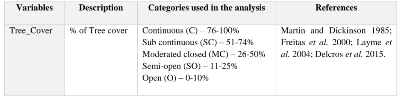
Table 3.1 – Environmental variables collected during the field work and used as candidate variables in the modelling
procedure. Values represent the percentage (%) of each variable within the 5m buffer centered on the ink tunnel. Variables Description Categories used in the analysis References
Tree_Cover % of Tree cover Continuous (C) – 76-100% Sub continuous (SC) – 51-74% Moderated closed (MC) – 26-50% Semi-open (SO) – 11-25% Open (O) – 0-10%
Martin and Dickinson 1985; Freitas et al. 2000; Layme et
7
Shrub_Cover % of Shrub cover Continuous (C) – 76-100% Sub continuous (SC) – 51-74% Moderated closed (MC) – 26-50% Semi-open (SO) – 11-25% Open (O) – 0-10%
Dueser and Shugart 1978; Martin and Dickinson 1985; Dunstan and Fox 1996; Ecke et
al. 2002; Delcros et al. 2015;
Layme et al. 2004; Kelt et al. 2004.
Grass_Cover % of Grass cover Continuous (C) – 76-100% Sub continuous (SC) – 51-74% Moderated closed (MC) – 26-50% Semi-open (SO) – 11-25% Open (O) – 0-10%
Bond et al. 1980; Martin and Dickinson 1985; Monadjem 1997; Layme et al. 2004.
Naked_Soil % of Naked soil 1 – 76-100% (open) 2 – 51-74% 3 – 26-50% 4 – 11-25% 5 – 0-10% (closed)
Bond et al. 1980; Martin and Dickinson 1985; Dunstan and Fox 1996; Delcros et al. 2015.
Tree_Height Height of trees High (H) - >20m Tall (T) – 10-20m Short (S) – 5-10m Low (L) – 2-5m
Dueser and Shugart 1978; Holland and Bennett 2009.
Shrub_Height Height of shrubs High (H) – 2-5m Tall (T) – 1-2m Short (S) – 0,5-1m Low (L) – <0,5m
Monadjem 1997; Hoffman and Zeller 2005; Holland and Bennett 2009.
Grass_Height Height of grasses High (H) - >2m Tall (T) – 1-2m Short (S) – 0,5-1m Low (L) – <0,5m
Monadjem 1997; Layme et al. 2004; Holland and Bennett 2009; Delcros et al. 2015.
Table 3.2 – Environmental variables collected during the field work, using camera-trapping, and used as candidate variables
in the modelling procedure.
Variable Description Mean / Range Resolution Source References
DIST Distance to houses 2738.97/30.8-9866.9 metres Collected at point
Camera-trapping survey Dunstan and Fox 1996.
HUMANS Capture rate
of humans in CT
0.84/0-10 Collected
at point
Camera-trapping survey
DOG Capture rate
of dogs in CT
0.175/0-3.02 Collected at point
Camera-trapping survey
CAT Capture rate
of cats in CT
0.05/0-0.5 Collected
at point
Camera-trapping survey
Class 1 Capture rate
of ungulates
0.397/0-3.04 Collected at point
Camera-trapping survey Keesing 1998; Hoffman and Zeller 2005; Rautenbach 2013.
Class 2 Capture rate
of ungulates
0.651/0-2.90 Collected at point
Camera-trapping survey
Class 3 Capture rate
of ungulates
0.103/0-1 Collected
at point
Camera-trapping survey
Class 4 Capture rate
of ungulates
0.119/0-0.83 Collected at point
8
Table 3.3 – Categories used to describe the abundance of wild ungulates detected during the camera-trapping campaigns.
Resulting variables were used as candidate variables in the modelling procedure.
3.4. Variables collected from remote sensing products
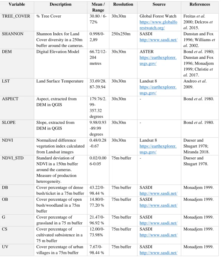
I selected remote sensing variables that were highlighted as important to rodents’ occurrence in previous studies focused on small mammals: (i) Normalized Difference Vegetation Index (NDVI), which allowed us to describe seasonal variations in vegetation and is therefore widely used as a vegetation productivity proxy (Glass et al. 2000; Andreo et al. 2009, Mapelli and Kittlein, 2009); (ii) Altitude, slope and terrain orientation, to describe the physical component of the habitat and because influences smaller scale heterogeneity, leading to higher microhabitats diversity (Schulze et al. 1997; Venturi et al. 2004; Fischer et al. 2011); (iii) Land use types and cover (proportion per buffer), allowing to translate landscape complexity (Goodin et al. 2006) through the calculation of a diversity index (ex. Shannon); (iv) Land Surface Temperature (LST), defined as the thermal emission of the soil, which varies according to soil cover, with the highest temperatures being registered in areas of bare soil, being a good indicator of the habitat cover structure (Andreo et al 2009).
In total, thirteen predictors (Table 3.4) were selected and data for the study area extracted and stored in a Geographic Information System (GIS). Most of the variables used have the resolution of 30x30m. The Shannon Index was calculated based on a land cover raster with a resolution of 30x30 meters. In order to capture habitat heterogeneity, the Shannon Index was calculated with a coarser resolution than 30x30 meters, resulting in a resolution of 250x250m. This resolution, besides covering at least 5 pixels of the land cover raster allowing to calculate diversity, is a measure that ensure that areas used by individuals for daily foraging activity and small-scale movement are included (Barrett and Peles 1999). The standard deviation of the NDVI (NDVI_STD) was calculated based on the NDVI. Land use classes (DB, OB, G, CS, UV) were also derived from the land use raster and were chosen because they are the land uses with greater representativeness in each of the study areas (i.e. Phinda Game Reserve, Livestock/Game Farms and Zulu Tribal Land). Buffer zones for land cover classes were described quantitatively through the calculi of the percentage of cover of each habitat feature within each area (Pearson 1993). The resolution of a 75 metre buffer, for NDVI_STD and land cover classes was chosen for the same reason as described before, but in this case I was able to choose a better resolution to capture
Categories Species Weight References
Class 1 Grey duiker (Sylvicapra grimmia), Red duiker (Cephalophus natalensis), Suni (Neotragus
moschatus), Steenbook (Raphicerus campestris)
4-25kg Keesing 1998; Hoffman and Zeller 2005; Rautenbach 2013. Class 2 Nyala (Tragelaphus angasii), Warthog (Phacochoerus
africanus), Impala (Aepyceros melampus), Bushbig
(Potamochoerus larvatus), Common Redbuck
(Redunca redunca)
45-150kg
Class 3 Zebra (Equus quagga), Wildebeest (Connochaetes
taurinus), Great Kudu (Tragelaphus strepsiceros),
Buffalo (Syncerus caffer), Waterbuck (Kobus
ellipsiprymnus)
120kg-600kg
Class 4 Giraffe (Giraffa camelopardalis), Elephant (Loxodonta
africana), Black Rhino (Diceros bicornis), White
Rhino (Ceratotherium simum), Hippopotamus (Hippopotamus amphibius)
9 the percentage of habitat and NDVI variation and avoid conflicting with the habitat diversity captured by the Shannon Index (Barrett and Peles 1999).
For categorical variables, histograms were drawn to detect the representativeness of each category within each variable (ex. High for shrubs height). Categories with represented by 5% or less were merged in order to reduce variability introduced in the model.
Table 3.4 - Environmental variables from geographic information systems (GIS), used as candidate variables in the modelling
procedure.
Variable Description Mean /
Range
Resolution Source References
TREE_COVER % Tree Cover 30.80 /
6-72%
30x30m Global Forest Watch
https://www.globalfo restwatch.org/
Freitas et al. 2000; Delcros et
al. 2015.
SHANNON Shannon Index for Land
Cover diversity in a 250m buffer around the cameras.
0.998/0-2,89
250x250m SASDI
http://www.sasdi.net/
Dunstan and Fox 1996; Williams et
al. 2002.
DEM Digital Elevation Model
66.72/12-204 metres 30x30m ASTER https://earthexplorer. usgs.gov/ Bond et al. 1980; Dunstan and Fox 1996; Monadjem 1999; Christie et
al. 2017.
LST Land Surface Temperature 33.69/28.
87-39.94 30x30m Landsat 8 https://earthexplorer. usgs.gov/ Andreo et al. 2009.
ASPECT Aspect, extracted from
DEM in QGIS 179.76/2. 99-357.32 degrees 30x30m - Bond et al. 1980.
SLOPE Slope, extracted from
DEM in QGIS
9.98/0.93 -89.99 degrees
30x30m - Bond et al. 1980.
NDVI Normalized difference
vegetation index calculated from Landsat images
0.48/0.28 -0.67 30x30m Landsat 8 https://earthexplorer. usgs.gov/ Dueser and Shugart 1978; Miranda 2018.
NDVI_STD Standard deviation of
NDVI in a 150m buffer around the cameras. Measure of production heterogeneity.
0.02/0.00 6-0.05
75m buffer - Dueser and
Shugart 1978.
DB Cover percentage of dense
bush/ticket in a 75m buffer 43.22/0-98.44 % 75m buffer SASDI http://www.sasdi.net/ Monadjem 1999.
OB Cover percentage of open
bush/woodland in a 75m buffer 14.80/0-77.20 % 75m buffer SASDI http://www.sasdi.net/ Monadjem 1999. G Cover percentage of grassland in a 75 m buffer 21.47/0-96.92 % 75m buffer SASDI http://www.sasdi.net/ Monadjem 1999. CS Cover percentage of cultivated subsistence in a 75 m buffer 12.00/0-73.98% 75m buffer SASDI http://www.sasdi.net/ Monadjem 1999.
UV Cover percentage of urban
villages in a 75m buffer 7.67/0-98.44 % 75m buffer SASDI http://www.sasdi.net/ Monadjem 1999.
10
3.5. Data analyses/modelling
3.5.1. Influence of environmental variables on rodents’ abundance
To detect multicollinearity between all independent variables, I estimated the variance inflation factor (VIF) from “fmsb” package (Nakazawa 2018), using the criteria of VIF < 5 for non-collinearity (Ringle et al. 2015).
The influence of environmental variables on rodents’ relative abundance was tested using a boosted regression trees (BRT) approach, built with the “gbm” package (Ridgeway 2004). This technique encompasses the advantages of regression trees (e.g. predictor variables can be of any type, analysis is insensitive to outliers and can accommodate missing data, Elith et al. 2008), overcoming their low predictive capacity through the boosting algorithm. The final model is a linear addition of several regression models in which the simplest term is a tree (De’ath 2007; Elith et al. 2008).
BRT models are resilient to model overfitting but, to have a better predictive performance, the model input parameters were defined (Carslaw and Taylor 2009). In BRT, learning rate is the shrinkage parameter that controls the contribution of each tree to the model and tree complexity determines the number of nodes in a tree and consequently its size. These two parameters control the number of trees in the model, while the bag fraction determines stochasticity by selecting the proportion of data being used at each step (Elith et al. 2008; Carslaw and Taylor 2009; Williams et al. 2010). All models were fitted to allow interactions using a ten-fold cross validation to determine the optimal number of trees for each model. The largest learning rate (lr) and the smallest tree complexity (tc) were selected in order to allow a minimum of 1000 trees in the BRT fitting process (see Elith et al. 2008). As the response variable (rodents’ abundance) has a normal distribution, analyses were based on a Gaussian function. Non-informative variables were removed during the fitting process, allowing the simplification of the set of variables (Elith et al. 2008). That simplification consisted in defining how many variables the function can test to remove, based on relative influence and total number of variables. Then, a graph was produced showing differences in the predicted deviance according to several scenarios, each one with a different number of variables removed. Next, I decided the number of variables to eliminate, and they were removed in order of minor relative influence. The final relative influence of each variable was calculated through a BRT. Relative influence measures are calculated by averaging the number of times a covariate is used for splitting, weighted by the squared improvement to the model as the result of each split. It is then scaled so the values sum to 100 (Colin et al. 2017). Fitted values were plotted in relation to the most important predictors, revealing their effects on rodent’s abundance. Explained deviance was calculated using the following formula from Abeare (2009).
𝐷2= 1 − (𝑟𝑒𝑠𝑖𝑑𝑢𝑎𝑙 𝑑𝑒𝑣𝑖𝑎𝑛𝑐𝑒 𝑡𝑜𝑡𝑎𝑙 𝑑𝑒𝑣𝑖𝑎𝑛𝑐𝑒 )
Confidence intervals of 95% were estimated for the fitted function of each variable by taking 500 bootstrap samples of the input data, with the same size as the original data and randomly selected with replacement. A boosted regression tree was fitted to each sample and the percentiles of five and ninety-five were calculated for the points of each function. All analyses were done using the software R Studio Version 1.1.463 (R Core Team 2017; RStudio Team 2015).
Models were implemented for each study area (Phinda, Farms, Rural Communities) aiming to compare the effect of environmental variables in rodent’s abundance in the different management areas. To assess the level of the effects of remote sensing variables, I produced BRT models using variables collected at sampling points, and mean values collected in a 75 metres buffer. Those that had higher influence on rodents’ abundance, were selected to perform the final model for each group and each area.
11 This was tested because, since I am working with GIS variables, sometimes the original resolution may not be the scale at which environmental variables affect the organism. In this case, I chose 75 metres according to Barrett and Peles (1999), as referred above. Since abundances meet the assumptions of normality according to Shapiro-Wilk normality test, there was no need to transform the data.
3.5.2. Spatial patterns of rodents’ abundance across areas and functional groups
Differences in mean abundance and standard deviation values of functional groups according to area (Phinda Game Reserve, Livestock/Game Farms and Zulu Tribal Land) were tested using an ANOVA and, if significant, a Tuckey HSD test.
In order to assess the occupancy patterns of rodents’ abundance within each area (i.e. aggregate, random/regular pattern), I evaluated the data using Lloyd’s Index of Patchiness (Lloyd 1967) for each of the three types of lands with distinct management schemes (i.e. Phinda Game Reserve, Livestock/Game Farms and Zulu Tribal Land). Using the QGIS Landscape Analysis tool (QGIS Development Team), Shannon Diversity Index was calculated for each of the study areas, in order to obtain a characterizing metric of the heterogeneity level.
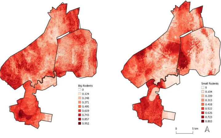
To identify spatial distribution patterns, gridded maps of each point-centred environmental predictor were developed and interpolated using the Kernel Density Estimation through “as.owin” function from package ”maptools” (Bivand et al. 2019) and “ppp” and “smooth.ppp” functions from package “spatstat” (Baddeley et al. 2019). Remaining variables were already in raster format, so there was no need to interpolate values. All variables were imported to R Studio and then, the fitted BRT model was used to predict the probability of occurrence in the entire study area. A different BRT model was used for each of the management systems, as previously described.
To test if the predicted values were accurate, I tested differences between mean and standard deviation values between original and predicted values, using a Welch Two Sample t-test or Wilcoxon-Mann-Whitney Test if values were not parametric, and Levene Test, respectively.
4. Results
4.1. Multicollinearity between independent variables
Analysing the Variance Inflation Factor (VIF) for all the independent variables, only Land Surface Temperature showed a value greater than 5 (collinearity) in Farms and Phinda, and was removed from the following analytical procedure. Others were also removed from the analysis, since no spatial variation was detected: Cattle (Phinda), and Class 2 and Grass Height (Rural Communities).
4.2. Drivers of abundance
4.2.1. Big Rodents
For big rodents, models for Phinda and Farms had a predictive deviance of 54 % and 67%, respectively, indicating a higher model robustness comparing to Rural Communities with just 26%.
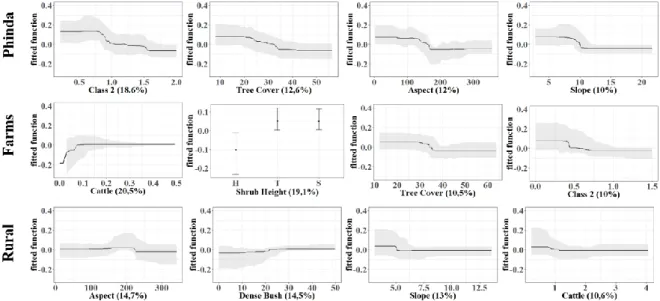
In Phinda, the group of variables most strongly influencing abundance were wild ungulates (Class 2), tree cover, aspect and slope (Figure 4.1). Big rodents are, therefore, more abundant where there are low capture rates of wild ungulates, slopes until 10 degrees and oriented east, and tree cover lower than 35%.
For farms, influence of cattle, shrub height, tree cover and wild ungulates (Class 2) was detected (Figure 4.1) on big rodents’ abundance. Thus, rodents occur most frequently in areas with lower abundances of wild ungulates, but avoided areas with shrubs over two meters, and with more than 35%
12 of tree cover. Despite cattle’s relative importance being high (20.5%), care must be taken in interpreting these results because the confidence intervals of this variable ranges from positive to negative values, preventing a confident interpretation of the true effect of livestock in big rodents.
Finally, for Rural Communities, drivers shaping big rodents’ abundance variation were similar to those identified for the other two areas (Figure 4.1). Aspect and slope had both a negative influence, indicating the same trend previously described. A relation with cattle rises in this analysis as an important factor, but again its confidence intervals range from positive to negative values, hampering the interpretation.
Figure 4.1 - Function fitted for the most important predictors by a boosted regression tree (BRT) relating the abundance of big
rodents to each environmental variable. Three model results are represented, one for each management type area: Phinda Reserve, Farms and Rural Communities. Important predictors are those whose relative importance is above 10%. Confidence intervals of 95% are represented in grey. Functions are continuous for all the variables except for shrub height, that consists in discrete values for each level of the factor predictor (H-high, T-tall, S-small). A common scale is used on the vertical axis for all plots
4.2.2. Small Rodents
For small rodents, Rural Communities and Phinda models had the best explained deviance, with 70 % and 52%, respectively. Farms had a lower performance, with only 30%.
In Phinda, small rodents’ abundance was again positively influenced by lower capture rates of wild ungulates (both classes). However, NDVI and DEM are also important drivers, with abundance being promoted by high values of productivity (i.e. NDVI) but constrained in lower altitudes (<80m).
For farms, small rodents seem to be influenced by both classes of wild ungulates (Class 1 and 2; Figure 4.2), showing a preference for areas with low abundances. Cattle showed once more a poor performance, with confidence intervals hindering interpretation of the influence pattern (Figure 4.2). For this reason, this variable will not be considered as influential for the farms’ dataset.
For Rural Communities, the most important variables were once more DEM and wild ungulates (Figure 4.2). Small rodents showed higher abundances in zones with low capture rates of ungulates and above 50 meters of altitude.
13
Figure 4.2 - Function fitted for the most important predictors by a boosted regression tree (BRT) relating the abundance of
small rodents to each environmental variable. Three models are represented, one for each management area: Phinda Reserve, Farms and Rural Communities. Important predictors are those whose relative importance is above 10%. Confidence intervals of 95% are represented in grey. A common scale is used on the vertical axis for all plots.
4.3. Spatial patterns of rodents’ abundance across areas and functional groups
Of the 196 sampling points, four had to be discarded from the analysis, due to the disappearance of the cameras or of the ink tracking tunnels (two from Phinda and two from Rural Communities). From the 192 sampling points monitored, 163 presented small rodents’ tracks, while 145 had big rodents’ tracks, with an overlap in 67 sites. Abundances of both rodents’ groups were significantly normal (Small: W=0.93, p-value<0.001; Big: W=0.88, p-value<0.001). Relative abundances of small and big rodents differed between areas (Figure 4.3). For small rodents significant differences were found between abundances at each of the three study zones (F (2.189) = 16.02, p<0.001). Post hoc comparisons using Tukey HSD test indicated that mean score for Phinda (M= 0.52, SD= 0.31) was significantly different (p<0.001) than the other two areas (Farms: M=0.31, SD=0.26; Rural: M=0.26, SD=0.26), with
Figure 4.3 - Boxplot of rodents’ relative abundance in the three management types zones monitored: Farms, Phinda reserve
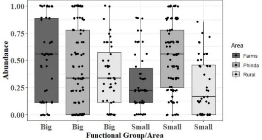
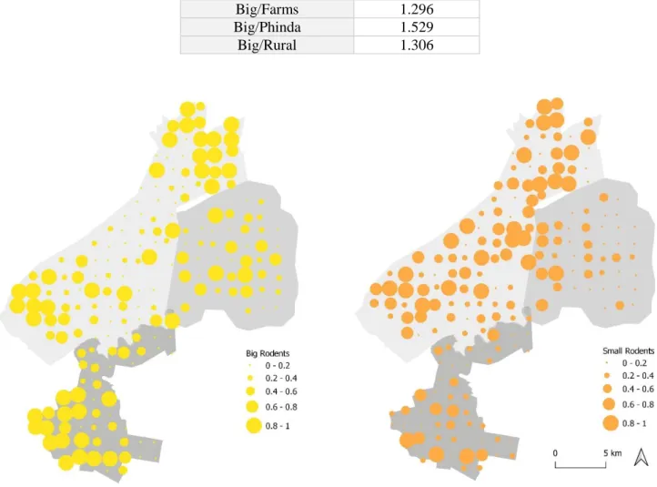
14 higher abundance values (Figure 4.3). For big rodents no significant differences were found between areas, but farms appear to hold a higher abundance comparing to the other areas (Figure 4.3). Only for Farms, abundances of big (M=0.52, SD=0.37) and small rodents (M=0.31, SD=0.26) were significantly different (p=0.001) Based on these results, each rodent functional group was analysed separately. Lloyd’s Index of Patchiness revealed that for every area and both groups, rodents’ abundance values were significantly aggregated (ℽ > 1) as it is possible to verify in Table 4.1. Through Figure 4.4 I intend to illustrate the patterns of rodent abundance, so that it is possible to visualize the areas with the highest aggregation levels of each group.
Table 4.1 – Results of Lloyd’s Index of Patchiness (ℽ).
Figure 4.4- Map of the study area showing both rodents’ distributions: big rodents in yellow and small rodents in orange. The
size of each point is equivalent to abundance value, as indicated in the respective legend Functional Group/Area Lloyd’s Index of
Patchiness (ℽ) Small/Farms 1.372 Small/Phinda 1.128 Small/Rural 1.528 Big/Farms 1.296 Big/Phinda 1.529 Big/Rural 1.306