Analysis of Usage Patterns of Medical Image Exams in Medical Environments

(1)

F

ACULDADE DE

E

NGENHARIA DA

U

NIVERSIDADE DO

P

ORTO

Analysis of usage patterns of medical

image exams in medical environments

Nuno Martins Marques Pinto

Mestrado Integrado em Engenharia Informática e Computação Supervisor: Luís Filipe Pinto de Almeida Teixeira Co-Supervisor: Vera Lucia Miguéis Oliveira e Silva

Company Supervisor: António Cardoso Martins

(2)

(3)

Analysis of usage patterns of medical image exams in

medical environments

Nuno Martins Marques Pinto

Mestrado Integrado em Engenharia Informática e Computação

Approved in oral examination by the committee:

Chair: Carlos Manuel Milheiro de Oliveira Pinto Soares External Examiner: Inês de Castro Dutra

Supervisor: Luís Filipe Pinto de Almeida Teixeira

(4)

(5)

Abstract

The increasing technological developments, the significant increase in healthcare data and the lack of knowledge regarding such data, have raised serious concerns regarding medical examinations’ management.

There are three distinct information systems, Hospital Information System, Radiology Infor-mation System and Picture Archive and Communications System (PACS) in a healthcare organi-zation. In the standard workflow, after the image acquisition by the imaging modality, the image is sent and stored in PACS where it can be remotely accessed by any authorized medical staff. In Portuguese public hospitals there is not much information regarding to which cases the ex-ams are consulted, by which doctors nor their specialties, neither for any specific purposes. The lack of information and analytic tools related to these issues are among the major concerns of the Portuguese health system stakeholders.

These problems can be tackled with the implementation of systems such as Business Intelli-gence allied with analytic techniques - cluster analysis and mining association rules. Therefore, in this work we intend to obtain groups of medical services of a hospital, according to its accesses to examinations’ pattern, during a 112-day period. These groups were obtained by performing a cluster analysis on the data set of similar medical services, with the clusters corresponding to the targeted segments. In addition to that, association rules mining were also performed in order to uncover associations between the multiple examinations’ characteristics, the specific medical services that access them and their visualization patterns.

In the end, this study enables to obtain homogeneous segments, which refer to the usage patterns of the medical services, and association rules that translate the relationships among the different components.

(6)

(7)

Resumo

Com a crescente evolução tecnológica, o aumento significativo da quantidade de dados relativos à saúde e a falta de conhecimento sobre os mesmos, criam-se sérias preocupações relativamente à gestão de exames médicos. Assim, devido a este crescimento a análise desses mesmos dados tornou-se ainda mais complexa e de difícil execução.

Num sistema hospitalar existem três sistemas de informação distintos, designadamente, o Hos-pital Information System, o Radiology Information System e o Picture Archive and Communica-tions System(PACS). No workflow tradicional, após a aquisição de imagens por parte da modali-dade, estas são enviadas e armazenadas no PACS onde podem ser acedidas remotamente por pes-soal médico devidamente autorizado. Nos hospitais públicos portugueses existe pouca informação referente em que casos os exames são ou não consultados, por que médicos, de que especialidades e com que intuito. A falta de informação e de ferramentas de suporte relativas a esta problemática estão entre as principais preocupações dos intervenientes do sistema de saúde português.

Estes problemas podem ser colmatados com a implementação de sistemas, tal como Business Intelligence, aliados a métodos analíticos - análise clustering e regras de associação.

Posto isto, neste trabalho pretende-se obter uma segmentação de um conjunto de serviços médicos de um hospital, de acordo com o seu padrão de acesso às imagens médicas dos exames, durante um periodo de 112 dias. Esta segmentação foi obtida efetuando uma análise cluster no conjunto de serviços médicos em estudo, correspondendo os clusters aos segmentados pretendidos. Para além disso, efetuou-se também uma exploração das regras de associação, com o objetivo de encontrar associações entre as variadas características dos exames médicos, os serviços médicos a que os acedem e os seus padrões de visualização. Assim, estas estratégias permitiram-nos obter segmentos homogéneos que traduzem os perfis de utilização dos múltiplos serviços médicos, e regras de associação que traduzem as relações entre as mais variadas componentes.

(8)

(9)

Acknowledgements

Always in first place, would like to dedicate this dissertation to all my family for supporting my moody days and nights, my rights and wrongs, and for teaching me every single day that at the end of the road through all the adversity, if you can get where you wanted to be, you remember whatever doesn’t kill you make you stronger, and all of the adversity was worth it.

To all my loyal and longtime friends, a huge thanks for bringing joy, happiness and childish moments to my life.

A very special thanks to my supervisors Luís Teixeira and Vera Miguéis, for the incredible guidance, partnership and availability. You were flawless.

Last but not least, I would like to express my sincere gratitude to António Martins and Carlos Cardoso for allowing me to be part of such an amazing project and team in an extraordinary environment. Also, a huge thanks to my Sectra colleagues for every single laugh and lesson.

(10)

(11)

“Never stop learning, never stop grinding, never stop loving every single minute of your life”

(12)

(13)

List of Figures

2.1 Main workflow in a radiology department [tHE] . . . 7

2.2 Basic architecture BI framework . . . 8

2.3 Using K-means to find three clusters in sample data (page 498 [TSK06]). . . 14

2.4 Example of center-based density (page 528 [TSK06]). . . 15

2.5 Illustration of classification of points (page 528 [TSK06]). . . 15

2.6 Sample data set. . . 16

2.7 K− dist plot for the data set. . . 17

2.8 Cluster resulted from DBSCAN [TSK06]. . . 17

2.9 An example of itemsets representation [HGN00]. . . 20

2.10 Association rules types of algorithms [HGN00]. . . 20

2.11 Illustration of the Apriori Principle [TSK06]. . . 21

2.12 Illustration of the Apriori pruning using the confidence measure [TSK06]. . . 23

3.1 Proposed BI system architecture . . . 28

3.2 User data extraction script flow chart . . . 30

3.3 Flow chart of Log Parsing Script . . . 32

3.4 Pareto analysis of the number of accesses per medical service. . . 38

3.5 Distribution of the Access Interval. . . 38

3.6 Exam Code frequency. . . 39

3.7 Modality distribution. . . 39

3.8 Module distribution. . . 40

3.9 Distribution of the Report variable. . . 40

3.10 Frequency of examinations that were not accessed. . . 41

3.11 Frequency of the Modality of the exams not accessed by Radiologists superset. . 41

3.12 Frequency of Body Part variable in CR examinations not accessed by Radiologists superset. . . 42

3.13 Frequency of Body Part variable in US examinations not accessed by Radiologists superset. . . 42

3.14 Frequency of the Modality of the exams not accessed by Others physician superset. 43 3.15 Frequency of Body Part variable in CR examinations not accessed by Other physi-cians superset. . . 43

3.16 Frequency of Body Part variable in CT examinations not accessed by Other physi-cians superset. . . 43

3.17 Frequency of Body Part variable in US examinations not accessed by Other physi-cians superset. . . 44

3.18 Final dashboard designed for end users. . . 45

(16)

LIST OF FIGURES

4.2 Davies-Bouldin Index Graph. . . 49

4.3 Cluster distribution dashboard. . . 50

(17)

List of Tables

2.1 An example of market basket transactions. . . 18

2.2 An example of binary representation of the market basket transactions. . . 18

3.1 Required data for extraction. . . 29

3.2 Final schema of the data extracted. . . 33

3.3 Number of physicians IDs and number of accesses per medical service. . . 34

3.4 Measures that summarize the variable Physician ID and the number of accesses per medical service. . . 38

3.5 Measures that summarize the number of accesses per examination. . . 40

4.1 Value of the normalized variables by cluster and global average. . . 52

4.2 Number of the examinations by cluster and global average. . . 53

(18)

(19)

Abbreviations

AD Active Directory BI Business Intelligence BFS Breadth-First Search

CHUSJ Centro Hospitalar Universitário São João CT Computed Tomography

DFS Depth-First Search

DICOM Digital Imaging and Communication in Medicine DM Data Mining

DW Data Warehouse

EHR Electronic Health Record ETL Extract Transform and Load ETL Extract, Transform and Load FK Foreign Key

GDPR General Data Protection Regulation HL7 Health Level 7

HIPAA Health Insurance Portability and Accountability Act HIS Hospital Information System

HIT Health Information Technology KPI Key Performance Indicator MRI Magnetic Resonance Imaging

PACS Picture Archive and Communication System PHI Protected Health Information

PK Primary Key

(20)

(21)

Chapter 1

Introduction

1.1 Context and Problem

With the lightning fast technologies and its constant evolution, health information systems and healthcare data have been massively growing over the past years. As per Lloyd et al. [Min17], from 2013 to 2020 healthcare data is expected to grow 48 percent annually reaching more than 2 000 exabytes (2 000 000 000 terabytes) in 2020. However, due to this growth, the extraction, analysis and understanding of healthcare data has become an even more complex task.

Each year more than 6 million exams based on medical imaging are made for diagnostic pur-poses in Portuguese public hospitals [dS18]. Still, there is a huge lack of knowledge of their utilization patterns.

It is expected each exam to be consulted, after the acquisition of the medical imaging, by a radiologist that performs the diagnosis and elaborates the respective report, followed by another doctor’s consulting - typically a clinician (e.g. an orthopedist or a pediatrician). In Portugal, there is not much information regarding in which cases are the exams consulted, by which doctors, from what specialties and for what purpose. On the other hand, we have exams that are potentially consulted by non-medical staff, are never consulted and/or do not have a report.

In the Radiology department, we can distinguish two different information systems: Radiol-ogy Information System (RIS) is used for scheduling, patient tracking, results reporting and image tracking; Picture Archiving and Communication System (PACS) is used for storing and transmit medical images and reports. As previously stated, the data available in these two information systems has been significantly increasing, but there are no implemented processes capable of in-terpreting such data and turn it into meaningful data to help the decision making, which nowadays is considered a very valuable tool amongst hospital’s management personnel.

Several studies ran by Yichuan et al. [WKB18], Osama et al. [ACJ16] and Ishola et al. [Mur12] show that data analytic solutions, such as Business Intelligence (BI), effectively provide opera-tional and strategic improvements in healthcare. Along with it, a BI implementation allow the

(22)

Introduction

final users to access meaningful and useful information through simple and interactive data pre-sentation (dashboards, scorecards, charts, graphics and so on) [Zhe17].

As stated, the existence of large amounts of healthcare data brings new challenges. On one hand, in order to keep track of when exams are accessed and who accesses them, there is the need to create a data warehouse (DW). On the other hand, there is the need to identify utilization patterns of the exams, by grouping and segmenting them according to meaningful variables. Although there are multiple analytical techniques used for data segmentation, cluster analysis remains the most common and the most used procedure, being vastly used in utilization patterns’ identification and analysis [MP87,WQK+17,AFHC13]. Mining association rules also play an important role in data mining, being used for undercover relationships between data items within large data sets [AIS93,

AS94].

This work is made in cooperation with Sectra1and Centro Hospitalar Universitário São João (CHUSJ)2. Sectra is involved in the markets of healthcare and cybersecurity, being mostly known for development, deployment and support of imaging IT solutions. The main theme of the disser-tation was proposed by the company which, in turn, arose from the need to provide a solution to the problem of the insufficient healthcare data analysis in Portuguese public hospitals.

1.2 Motivation and Objectives

Our main purpose in this dissertation is to try to tackle the challenges described in the previous section 1.1 applying a custom BI framework, based on the standard one - Data Sources, Data Acquisition, Data Storage, Data Analysis, Data Visualization -, and applying data analysis tech-niques, clustering and mining association rules, to obtain exams’ visualization patterns. More specifically, develop an accurate system capable of:

1. Extracting data (structured, semi-structured and unstructured data) correctly from specific sources;

2. Processing heterogeneous data;

3. Anonymizing data classified as Protected Health Information (PHI); 4. Storing processed data in a proper data warehouse;

5. Segmenting data by applying cluster analysis;

6. Identifying relationships between data objects using association rules mining;

7. Interpreting and displaying analyzed data in several formats, promoting an interactive visu-alization.

1_{https://www.sectra.com/investor/about.html} 2_{http://portal-chsj.min-saude.pt/}

(23)

Introduction

To the best of our knowledge, there are no records of any study or work focusing on the utilization patterns of exams based on medical imaging. This dissertation has also the goals to successfully complete development, deployment and validation of this system.

1.3 Dissertation Structure

In addition to this chapter, the dissertation is composed by five other chapters:

• Chapter2introduces the theoretical aspects of all the subjects relative to this dissertation. This chapter starts with a brief history about the evolution of the healthcare information sys-tems until the present, then a review of the state-of-the-art of Business Intelligence, cluster analysis and the current data protection regulations (General Data Protection Regulation). • Chapter3 presents the methodology involved in the dissertation, including the proposed

solution and its subsequent implementation details;

• Chapter4describes and discusses the results obtained from our implemented cluster anal-ysis;

• Chapter5describes and discusses the results obtained from association rules mining; • Chapter6 summarizes the results of the whole dissertation and concludes with

(24)

(25)

Chapter 2

Background Knowledge

In this chapter different subjects related to the dissertation and to the implementation are ad-dressed. The first step is to understand which are the different healthcare information systems, how they communicate and what information is stored in each system. These systems are going to be the main data sources. Subsequently also to understand which of these systems are imple-mented in Portuguese public hospitals.

The second step is to understand the Business Intelligence architecture, its framework and how the integration with the information systems can be made. Since dealing with healthcare data which can be considered sensitive - as it may directly or indirectly identify an individual -, data anonymization is required under the General Data Protection Regulation (GDPR).

Lastly, a review of the data analysis techniques used is also presented.

2.1 Health Information Systems

Understand and distinguish the different data sources to be used, what information can be ex-tracted and how to extract from each source, is an essential first step of the project. Throughout this analysis it is possible to identify three main systems: Hospital Information System (HIS); Radiology Information System (RIS); Picture Archive and Communication System (PACS). Each system has different purposes although the same data can be found in more than one system, in result of the systems’ interaction.

In order to integrate and create interoperability between different health related systems, two protocols and standards were created. Digital Imaging and Communications in Medicine (DI-COM)1and Health Level 7 (HL7)2are the communication standards used in health information’s exchange. DICOM is used to transmit, store, process and display medical imaging information over a network (e.g. transfer Computed Tomography (CT) images to a remote storage), and HL7

1_{https://www.dicomstandard.org/}

(26)

Background Knowledge

is used to exchange, integrate, share and retrieve electronic health information (e.g. patient data) between medical software. While DICOM increases interoperability, HL7 decreases the incom-patibilities amongst the different medical applications. Both standards are the basis of the infor-mational integration of software based medical processes [COV+10,RA15].

HIS is the main management system in a hospital. It is responsible for administrative and financial management, stock management (e.g. medicines) and store Electronic Health Record (EHR) of patients, which contains patient personal data and patient medical history. Generally, the HIS communicates with RIS to share patient related data. In this project, data extraction from HIS will not occur.

RIS, like the name suggests, is used by the Radiology department to better manage processes and improve the workflow. RIS allows staff to keep track of patient’s workflow (e.g. patient doing a Magnetic Resonance Imaging (MRI)), scheduling appointments, do clinical reports, although nowadays it is usually done in PACS, and image management. Its advantage prevails on keeping data easily accessible turning into a more efficient workflow management [NMN13]. RIS obtains data related to patient from HIS via HL7 messages, and sends that information to the imaging modalities (e.g. CT scan) via DICOM when required.

Moreover, PACS is responsible for medical imaging storage and also has the ability to provide remote access to those images. PACS receives images from imaging modalities and the informa-tion related to patient, previously sent by RIS to the modality, and stores them in a virtual storage, via DICOM [O’C17,RA15]. In short, as pointed out by Carter et al. [CV10], a PACS serves as the file room, reading room, duplicator and courier, providing image access to multiple users at the same time. Therefore, in PACS data is stored relative to patients, exams, images, medical staff and so on. PACS will be the main data source of this project.

In summary, to better understand the schedule workflow in a radiology department, figure2.1

describes the typical workflow since patient examination’s schedule until the exam’s consulting by medical staff. The patient is registered, in HIS, and an examination requisition is made. This requisition is passed to RIS, where the exam’s confirmation is made and it is scheduled to a specific date. Then, when performing the examination, the images are acquired by the medical imaging modality and sent to PACS. As known, PACS will provide medical staff remote access to the images, allowing radiologist to analyze the images, make the diagnosis and write the respective report. The report will then be gathered with the patient’s EHR, being able to be consulted by any authorized medical staff.

2.2 Business Intelligence

Business Intelligence has been implemented for several purposes and it brought up significant improvements in healthcare. From providing medical staff tools for decision making, to provid-ing clinical Key Performance Indicators (KPI), BI has a wide range of applications combinprovid-ing data gathering, data storage, data integration and knowledge management with analytical tools to

(27)

Figure 2.1: Main workflow in a radiology department [tHE]

display key information for planners and decision makers [You18]. Furthermore, BI follows a spe-cific framework, as illustrated in figure2.2, that includes data management, analysis, presentation and delivery.

As pointed out by Sang [You18], Ali et al. [AÖNC13] and Mark Peco [Pec11], BI applica-tions in healthcare can be categorized in two major sets of soluapplica-tions, i.e. Business Soluapplica-tions and Technology Solutions.

Technology Solutions, consists on Data & Information Tools, are as follows:

• Decision Support Systems (DSS): Support managerial decision making, usually day-to-day tactical.

• Executive Information Systems: Support decision making at the senior management level which provide and consolidate metrics-based performance information.

• Online Analytical Processing (OLAP): Support analysts with the capability of performing multidimensional analysis of data.

• Query and Reporting Services: Provide quick and easy access to the data with predefined report design capabilities.

• Data Mining (Predictive Model as explained by Ali et al. [NCH11,NHC13,NCH12]): Ex-amines data to discover hidden facts in databases using different techniques.

(28)

Figure 2.2: Basic architecture BI framework

• Operational Data Services: Collect data from end users, organize data, establish solid data structures and store them in different databases, retrieve data from multiple databases. Business Solutions consists on business focused analytical applications, as follows:

• Patient Analysis: Focuses on analysis of patients’ demographic and satisfaction processes. • Electronic Health Record Analysis: Focuses on the analysis of the quality of clinical data. • Performance Analysis: Streamline and optimize the way that a business uses its resources. • Fund Channel Analysis: Devise, implement, and evaluate fund strategies, then use the

cor-porate metrics to continuously monitor and enhance the fund process.

• Productivity Analysis: Focuses on building business metrics for activities such as quality improvement, risk mitigation, asset management, capacity planning, etc.

(29)

• Behavioural Analysis: Understanding and predicting trends and patterns that provides busi-ness advantage.

• Supply Chain Analysis: Monitor, benchmark, and improve supply chain activities from materials ordering through service delivery.

• Wait Time Analysis: Focuses on the factors that are associated with longer waiting times and the effects of delays in scheduling and operation.

Regarding the purpose of the project and our scope, our methodology will be processed through data mining.

2.2.1 Data Management

The first step to implement a BI system is to define which external or internal data sources are going to be explored. Data management consists on identifying structured and unstructured data sources, and extract data to temporary data store systems or directly to the final Data Warehouse (DW). If the data is first stored in a temporary data system, it must be afterwards migrated to a proper DW. This migration only occurs after a proper definition and creation of the schema. Be-sides migrating information in this phase, data must be processed in order to obtain homogeneous data if required, since they were extracted from different sources and may be in different formats. This whole process is called Extract, Transform and Load (ETL). The ETL process may occur directly from the data sources or from temporaries data systems.

2.2.2 Data Analysis

As stated by Schniederjans et al. [SSS14] data analytics is defined as a process that involves the use of statistical techniques, information system software, and operations research methodologies to explore, visualize, discover and communicate patterns or trends in data. We can distinguish four types of data analysis:

• Descriptive: identifies patterns but does not point to any cause or explanation. • Diagnostic: identifies patterns and give insights into specific problems.

• Predictive: uncovers relationships and patterns within large volumes of data to detect ten-dencies [Eck09].

• Prescriptive: detect tendencies but suggests also actions to prevent future problems and the advantages of a promising trend.

Data analysis can be done throughout the use of multiple techniques, such as ad hoc queries or Data Mining (DM) techniques (e.g. classification or clustering) [KKS17]. In this dissertation, we will focus on the clustering techniques and on mining association rules.

(30)

2.2.2.1 Clustering

Clustering (or cluster analysis) is an exploratory technique that organizes a collection of patterns, usually represented as a point in a multidimensional space, into groups (clusters) based on simi-larity. Intuitively, patterns within a valid cluster are more similar to each other than they are to a pattern belonging to a different cluster [JMF99]. Being a data analysis technique, clustering can be used as a stand-alone tool that allows to obtain the clusters’ natural structure and its charac-teristics. It can also be used alongside other techniques, like classification, and may be a starting point for other purposes, such as data summarization [TSK06].

Cluster analysis techniques have been developed in an attempt to analyze even larger data sets. This was a result of the need to transform huge amounts of data into meaningful and useful infor-mation. Although data mining can be considered as the main origin of clustering, it is vastly used in other fields of study such as bioinformatics [MC05,ENBJ05] and machine learning [ZK04].

Until this day, there is not a consensual definition of cluster. In fact, there are many different definitions of cluster and its interpretations are so diversified that, although the broad nature of this concept may reveal positive aspects, once it is applied in different contexts, it can be considered rather vague and somewhat confusing [MS03].

There are many techniques for cluster formation what may lead to clusters with significant differences. As per Hand et al. [HSM01] these methods can identify structures in distinct groups, however it is not always transparent the description of the respective clustering algorithm. For instance, a cluster can be defined as a collection of objects where the maximum distance between every pair of objects is the smallest possible. In this case, a method that minimizes the distances between each pair of objects is applied. On the other hand, a cluster can be defined as a group of objects where each object is the closest to any other object of its group, not being necessarily close to the other members of the cluster. This way, the methods mentioned in first place would not be efficient to identify the second type of clusters.

In order to choose the technique for cluster formation, the real problem and the analysis goals must be taken into consideration. The analysis should not be limited by assumptions and we should look for new techniques and new clusters in order to possibly identify patterns that were not taken into account previously [HSM01].

In summary, the goal of clustering is to split the objects in groups, so that the objects in a group are closer to them than to the members of any other group. This way, we can guarantee that the method of the cluster formation depends on a distance measure between objects, and also between groups.

Although each cluster analysis has its specifics problems, features and goals, it is possible identify a sequence of steps. As per Jain et al. [JMF99,JD88] these five steps are:

1. Object representation (optionally including feature extraction and/or selection). 2. Definition of an object proximity measure appropriate to the data domain. 3. Cluster analysis.

(31)

4. Data abstraction (if needed). 5. Assessment of output (if needed). Object representation

Refers to the number of classes, the number of available objects, and the number, type, and scale of the features available to the clustering algorithm. On one hand, feature (or variable) extraction is the use of one or more transformations of the input features to produce new salient features. On the other hand, feature selection is the process of identifying the most effective subset of the original features to use in clustering. These techniques are used to obtain an appropriate set of features to use in cluster analysis.

This stage is the equivalent to data preprocessing in clustering, which also includes several procedures [HK06]:

1. Handling missing values: real data sets tend to be incomplete, contain noisy or inconsis-tent data. Data cleansing is the first step to complete missing values, reduce noisy data by detecting outliers and fix inconsistencies.

2. Integration: gather data from different sources, processing heterogeneous and eliminating redundancies.

3. Transformation: transformation of the variables (standardization, discretization and vari-ables’ construction) in order to improve algorithms efficiency and/or identify patterns. Stan-dardization is used when variables are in different units or scales and they are changed to the same unit, scale or format. Discretization is, sometimes, used in variables with low levels of abstraction (e.g. age), so that those variables are substituted with ones with high levels of abstraction (e.g. adult). Construction of new variables is used to better interpret and understand data and the relation between variables.

4. Data reduction: reduce data set size by cutting down the number of objects or the variables in study.

The analyst’s role in the object representation process is to gather facts and conjectures about the data, optionally perform variable extraction, and design the subsequent elements of the clus-tering system. The user also should decide which aspects are relevant in its particular problem and context. A good object representation can often yield a simple understood clustering, as a poor one may yield a complex clustering.

Object proximity

Consider that the data set has n objects, which may represent either a physical object (e.g. a car) or an abstract notion (e.g. a style of writing). Cluster analysis algorithms are mainly applied on two data sets [HK06]:

• Dissimilarity matrix: A nx n matrix where each entrance matches the dissimilarities between each pair of objects. Dissimilarity between two objects is a measure that represents the difference between those objects.

(32)

• Data matrix: A n x p matrix with n objects and p variables (X1, X2, ..., Xp) that define them.

Hereby, the dissimilarity is lower for a pair of objects more similar. The dissimilarity measure Dbetween object x1and object x2satisfies the following [Gos12]:

1. Non negativity: D(x1, x2) ≥ 0

2. Reflexivity: D(x1, x2) = 0 , x1= x2

3. Symmetry: D(x1, x2) = D(x2, x1)

4. Triangle Inequality: D(x1, x2) + D(x2, x3) ≥ D(x1, x3)

Choosing the right measure of dissimilarity depends on the type of variables - numerical and categorical. We will only focus on the numerical ones.

The Euclidean distance is commonly used to calculate the proximity of objects in two or three-dimensional space, being the most used metric. This distance measure can be defined as follows:

D2(xi, xj) = ( p

∑

k=1

(xi,k− xj,k)2)1/2 = ||xi− xj||2,

which, in turns, is a special case (q = 2) of the Minkowski metric

Dq(xi, xj) = ( p

∑

k=1

(xi,k− xj,k)q)1/q = ||xi− xj||q,

where p is a positive integer and xi = |xi,1, ..., xi,p| , | : i = 1, ..., n are the data set’s objects with

pvariables.

Another usual distance is the Manhattan distance, also known as City Block, usually compared to the Euclidean distance. Manhattan distance can be defined as follows:

D(xi, xj) = p

∑

k=1

|xi, k − xj, k| ,

If the variables have different significance, each variable assigned to a weight wi, we can use

the weighted Euclidean distance

D(xi, xj) = s p

∑

k=1 wi(xi,k− xj,k)2,

or also use the same weighted distance variation to the Manhattan or Minkowski [Gos12,

HK06,JMF99,SAW15,TSK06]. Cluster Algorithms

Cluster analysis includes a variety of techniques, each one used for a different purpose, as discussed before. There are innumerous distinct approaches, however in this work we only focus prototype-based and density-based clusters, i.e. K-means and DBSCAN respectively.

(33)

First and foremost, it is important to understand what is partitional clustering and what’s its difference from hierarchical clustering. Partitional clustering is a division of the set of data into non-overlapping clusters such that each data object is in exactly one subset, and hierarchical clus-tering is a set of nested clusters that are organized as a tree - each node (cluster) in the tree, except for the leaf nodes, is the union of its children, and the root of the tree is the cluster containing all the objects. Thus, the subsequent output clustering can be hard (a partition of the data into groups) or fuzzy (each object has a variable degree of membership in each of the output clus-ters) [JMF99,Kol01].

Partitional methods require prior knowledge of the number K of clusters and group all the object into those K clusters. These algorithms have advantages when used with large data sets. The objects in the same cluster should be similar while objects in different clusters should be different (be far away in a dimensional representation). The most known partitional methods are K-means, Kmedoids (or Partitioning Around Medoids) and its variations, which are based on prototypes -every object relative to a certain prototype is closer to it than to any other prototype. In K-means, the prototype is called centroid (the center of the cluster), while in K-medoids the prototype is called medoids. Unlike centroids, medoids must be an object in the data set [KJR90,HK06].

Besides being easy to implement, K-means is one of the most used algorithms, with time complexity of O(n ∗ k ∗ i) where n is the number of objects in K clusters and i is the number of iterations needed to find the optimum solution.

As explained by Pavel Berkhin [Ber02], Pang-Ning et al. [TSK06] and Jiawei Han et al. [HK06], the first step of K-means is to choose K initial centroids, each object is then assigned to the closest centroid, according to the Euclidean distance between the object and the centroid, and each group of objects assigned to its respective centroid is a cluster. The centroid of each cluster is then up-dated based on the mean value of its objects, and this process is repeated until there are no changes in the centroids (vide algorithm1).

Algorithm 1: K-means partitioning algorithm Choose K objects as initial centroids; while centroids change do

Assign each object to its closest centroid forming K clusters; Update the clusters’ centroids;

end

There are some variants of the K-means algorithm, which can differ on the selection of the number of clusters, on the proximity measure or on the objective function.

As a centroid-based partitioning technique, the center of a cluster is represented by a centroid. The dissimilarity between an object xjand a cluster’s centroid ciis measured by dist(xj, ci), where

dist(y, z) is the Euclidean distance between two points y and z. The objective function that mea-sures the quality of a cluster, is the sum of squared error between all objects in a cluster and its centroid ci. This measure can be defined as follows:

(34)

Background Knowledge SSE = k

∑

i=1x

∑

j∈Ki dist(xj, ci)2,

where SSE is the sum of the squared error for all objects in the data set, xj a given object and

cia centroid of cluster Ki. In short, for each object in each cluster, the distance from the object to

its centroid is squared and the distances are summed. The objective function is to make K clusters as compact and separate as possible [HK06].

A simple example of the K-means is shown in figure2.3, using the mean as the centroid. The crosses represent the centroids, the triangles, squares and circles the objects in a data set (similar shape in different objects means they are assigned to the same cluster). When the algorithm terminates, in iteration 4, the centroids have grouped its respective points.

Figure 2.3: Using K-means to find three clusters in sample data (page 498 [TSK06]).

On the other hand, density based algorithms are generally related to finding non-linear shapes structure clusters [RSJM10]. One of the most widely and used density based algorithms is DB-SCAN (Density-Based Spatial Clustering of Applications with Noise). DBDB-SCAN produces a par-titional clustering, in which the number of clusters is automatically determined by the algorithm. However, DBSCAN can not produce a complete clustering because points in low-density regions are classified as noisy data and are omitted.

Initially we must take into consideration the key notion of density. There are several distinct methods for defining density, like center-based approach on which DBSCAN is based. In this approach, density is estimated for a particular object in the data set by counting the number of objects within a specified radius of that object, including the object itself. An example of this approach is illustrated in figure2.4where the number of objects, within an E ps radius, of object A is seven [EFKS00,Kol01].

Thus, based on center-based approach, according to Pang-Ning et al. [TSK06] the objects can be classified as:

(35)

Figure 2.4: Example of center-based density (page 528 [TSK06]).

• Core points: if the number of objects, within a given neighborhood (with a certain radius), around the object exceeds a certain threshold (MinPts is the number of minimum points required as a point to be considered as core point). In the following example2.5object A is a core point, for a radius E ps if MinPts ≤ 7.

• Border points: is in a core’s point neighborhood but it is not classified as core point. In the following example2.5object B is a border point.

• Noise points: any object that is neither a core point nor a border point. In the following example2.5object C is a noise point.

Figure 2.5: Illustration of classification of points (page 528 [TSK06]).

Based on the previous settings, DBSCAN groups two core points that are close enough to each other, with a distance lower than its E ps. The same thing is applied with border points, every one that is close enough to a core point is assigned to the same cluster as the core point. Noise points do not belong to any cluster (vide algorithm2).

Algorithm 2: DBSCAN algorithm Classify all objects;

Discard noise points;

Match all core points with a distance from each other lower than a given E ps ; Assign different clusters to every matched core point;

(36)

In order to determine E ps and MinPts, the main approach used is to look at the distance from an object to its kthnearest neighbor, named k − dist. Considering all objects in a cluster, the value of k − dist will be small if k is not larger than the cluster size. This may differ depending on the cluster’s density and the distribution of the objects. For objects not assigned to a cluster (noise points) the k − dist will be large. So computing k − dist for all the data set for a given k, sort the objects in increasing order and then plot them, it is expected to observe an abrupt change of the k− dist value. Assuming this measure as E ps and the value of k as MinPts, then objects for which k− dist is less than E ps will be classified as core points, while the remaining are border or noise points [GT15].

Figures 2.6 and2.7 show an example of a data representation with the respective k − dist graph. Although the value of E ps depends on k, its change is not significant. It is crucial to give a right value to k. Giving a low value to k will incorrectly assign noise points as clusters and giving high value, then small clusters can be classified as noise. Generally, the default value of k is 4, which appears to be the most suitable value according to Ester et al. [EFKS00].

Figure 2.6: Sample data set.

To demonstrate the DBSCAN application, we will continue the previous example 2.6 com-posed by 3000 two-dimensional objects. The value of E ps was found by plotting the k − dist graph2.7and identifying the value when the abrupt change occurs (E ps = 10). Using this k value and MinPts = 4, the clusters resulted from the DBSCAN algorithm are illustrated in the following figure2.8. The crosses represent the noise, and all the different shapes represent each cluster.

(37)

Figure 2.7: K − dist plot for the data set.

Figure 2.8: Cluster resulted from DBSCAN [TSK06].

Although being capable of identifying many clusters that K-means could not do, DBSCAN algorithm has complications when clusters have varying densities or with high levels of multi-dimensional data, where densities are more difficult to define [Ber02,Kol01,EFKS00].

Data abstraction

This stage is sometimes included in the previous step. It includes a simplistic representation of the data set (e.g. plotting), promoting an intuitive comprehension and understanding of the patterns [DS76].

Assessment of output

Represents the evaluation of the output. Questions like "Are the clustering results good or poor? What characterizes a good clustering and a poor one?". Every cluster algorithm will produce clusters, however some clustering algorithms may produce better results depending on the context, on the data set and on the goal. The study of cluster tendency (vide Yizong Cheng [Che95]

(38)

and Richard Dubes [Dub87]) is used, prior to the cluster analysis, to examine the data set to check if there are meaningful clusters through statistical and visual analysis methods.

2.2.2.2 Association Rules Overview

Association rules are an important class of regularities within data which have been extensively studied by the data mining community. The general objective is to find frequent co-occurrences, called associations, of items within a set of transactions. According to Bing Liu [Liu06] the idea of discovering such rules is derived from market basket analysis, where the goal is to mine patterns describing the customer’s purchase behaviour. Table 2.1 illustrates an example of the market basket transactions, where each row corresponds to a transaction and a set of items bought by a given customer.

Transaction ID Items 1 {Rice, Bread} 2 {Rice, Apple, Beer, Eggs} 3 {Bread, Apple, Beer, Cookies} 4 {Rice, Bread, Apple, Beer} 5 {Rice, Bread, Apple, Cookies} Table 2.1: An example of market basket transactions.

Table2.2illustrates the binary representation of table2.1, where an item is treated as a binary variable whose value is 1 if the item is present in a transaction and 0 if it is not present. There are also methods for handling categorical and quantitative data, however we will only focus the binary representation [AIS93].

Transaction ID Rice Bread Apple Beer Cookies Eggs

1 1 1 0 0 0 0

2 1 0 1 1 0 1

3 0 1 1 1 1 0

4 1 1 1 1 0 0

5 1 1 1 0 1 0

Table 2.2: An example of binary representation of the market basket transactions.

The uncovered relationships can be represented as follows: {Apple}→{Beer}. This rule sug-gests that a strong relationship exists between the sale of apples and beers, because many cus-tomers who buy apples also buy beer.

Association analysis has widely range of applications domains such as retailing, Web mining, bioinformatics, medical diagnosis and scientific data analysis. When applying association analysis it is important to take into consideration that some discovered patterns are potentially spurious because they may happen just by chance [TSK06].

(39)

Problem Definition

The problem of mining association rules is stated as follows: T = {t1,t2, ...,tn} is a set of

trans-actions, where each transaction contains items of the item set I = i1, i2, ..., ik. Thus, an association

rule is an implication of the form: X → Y , where X is a set of some items in I (X ⊂ I) and Y is a single item in I (Y ⊂ I) that is not present in X (X ∩ Y = 0). The strength of an association rule can be measured in terms of its support, confidence and lift. Support indicates how often a certain rule is applicable to a given data set

Support, s(X → Y ) = σ (X ∪ Y ) N

where σ (X ∪ Y ) is the support count - number of transactions which contain X and Y - and N is the total number of transactions. Confidence determines how frequently items in Y appear in transactions that contain X

Con f idence, c(X → Y ) = σ (X ∪ Y ) σ (X )

where σ (X ) is the number of transactions that contain X . Lift is simply the ratio of these values: target response divided by average response.

Li f t(X → Y ) = Support(X ∪Y ) N Support(X ) N ∗ Support(Y ) N

Generally, if the lift value is greater than one then X and Y are positively correlated. If the lift is less than one then X and Y are negatively correlated [AIS93,HGN00].

For instance, considering the rule {Bread, Apple}→{Beer} the support count for {Bread,Apple,Beer} is 2 and the total number of transactions is 5, so the rule’s support is 2/5 = 0.4. The rule’s confidence is obtained by dividing the support count for {Bread,Apple,Beer} by the number of transactions that contain {Bread,Apple}. So, the confidence for this rule is 2/3 = 0.67.

As stated by Pang-Ning et al. [TSK06], these measures interpretation is crucial to understand if a rule is interesting or not, if a rule happens by chance or not. When a rule has very low support it may occur simply by chance, and it is also an indicator of low significance. For these reasons, support is often used to eliminate uninteresting rules. On the other hand, confidence measures the reliability of the inference by a rule, what means the higher the confidence, more likely it is for Y to be present in transactions that contain X .

As per Agrawal et al. [AIS93] mining association rules can be divided in two major subtasks: 1. Discover frequent itemset: whose objective is to find all itemsets that are greater or equal

than a given support value - called minimum support (minSup).

2. Rule Generation: whose objective is to extract all the rules, with high confidence values, from itemsets found in the previous step.

(40)

Is known that the computational requirements are much more expensive for the search of frequent itemset than those for rule generation.

Apriori Algorithm

Since the introduction of the Apriori Algorithm, several algorithms focusing either frequent items’ search or rule generation, have been proposed [AIS93]. However, Apriori provides solution for both problems.

Figure 2.9: An example of itemsets representation [HGN00].

In figure2.9, the bold line represents the border between frequent and infrequent itemsets. All items above the border fulfill the minimum support requirements called frequent itemsets -while the ones bellow the line do not fulfill such requirements - called infrequent itemsets. The algorithm has the goal to determine that line in order to find the frequent itemsets.

Figure 2.10: Association rules types of algorithms [HGN00].

There are two types of association rules algorithms: i.e. Breadth-First Search (BFS) and Depth-First Search (DFS) [HGN00]. In BFS algorithms, such as Apriori, the value of support for

(41)

each itemset is determined for each specific level of depth, whereas DFS recursively descends the graph. Mining association rules algorithms can be summarized as shown in figure2.10.

The Apriori principle defines that if an itemset is frequent, then all of its subsets must also be frequent. Conversely, if an itemset is infrequent, then all of its supersets must be infrequent too. In the following figure2.11, we can observe the these two theorems. Assuming {c,d,e} is a frequent itemset, then its subsets ({c,d},{c,e},{d,e},{c},{d},{e}) are also frequent. On the other hand, if a itemset {a,b} is infrequent, then all the itemsets containing {a,b} are infrequent and can be discarded immediately [TSK06].

Figure 2.11: Illustration of the Apriori Principle [TSK06].

Concerning the discover of frequent itemset, in the first place every item is considered a 1-itemset candidate. Using the market basket example and using support threshold of 60% (min-Sup=0.6), after determining the support value for each candidate, {Cookies} and {Eggs} are dis-carded because they appear in less than 3 transactions -i.e. 0.6 ∗ 5 = 3. In next iteration, 2-itemsets candidates are generated using only the frequent 1-itemsets ({Rice},{Bread},{Apple},{Beer}), due to the infrequent theorem. Because there are four frequent 1-itemsets, the number of 2-itemsets candidates generated by the algorithm is (4₂) = 6 - {Beer,Rice}, {Beer,Apple}, {Beer,Bread}, {Rice,Apple}, {Rice,Bread}, {Apple,Bread}. Two these six candidates ({Beer,Rice},{Beer,Bread}) are also labeled as infrequent because their support count is two. Without the pruning method there are (6

3) = 20 3-itemset candidates, with the Apriori principle, as we only consider 3-itemsets

whose subsets are frequent, there is only one 3-itemset candidate - {Rice,Apple,Bread}. A bruce-force strategy of enumerating all itemsets will produce

(42)

candidates. Applying the Apriori principles, this number decreases massively to (6₁) + (4₂) + 1 = 13

candidates, which means a 68% reduction in the number of candidates [AS94,CR06]. This Apriori algorithm is described, in detail, in the following pseudocode.

Algorithm 3: Apriori Algorithm pseudocode k=1 ,{Find all frequent 1-itemset};

Fk= (i|i ∈ I ∧ σ (i) ≥ N ∗ minSup;

while Fk6= 0 do

k = k+1;

Ct = apriori − gen(Fk−1) ,{Generate itemsets candidates} ;

for each transaction t ∈ T do

Ct = subset(Ck,t) ,{Identify all candidates that belong to it} for each candidate

itemset c∈ Ct do

σ (c) = σ (c) + 1 ,{Increment support count}; end

end

Fk= {c|c ∈ Ck∧ σ (c) N ∗ minSup} ,{Extract the frequent k-itemsets}

end

Result = ∪ Fk

The apriori-gen function is the one responsible for grouping the itemsets into new itemsets, with one more item than the previous itemset, and removing the infrequent itemsets. The candi-dates are being stored in a hash-tree, where each node contains an itemset candidate. The subset functions starts from the root node going towards the leaf nodes in order to find all the candidates contained in a given transaction t.

Regarding generating association rules in Apriori algorithm, each frequent k-itemset, Y , can produce up to 2k− 2 association rules, discarding rules with empty antecedents or consequents (0→Y or Y→0). An association rule can be extracted by partitioning the itemset Y into two non-empty subsets X → Y and Y − X , such that X → Y − X satisfies the confidence threshold (e.g. as-sume Y ={1,2,3} is a frequent itemset, so six candidates can be generated {1,2}→{3}, {1,3}→{2}, {2,3}→{1}, {1}→{2,3}, {2}→{1,3} and {3}→{1,2}, discarding afterwards the ones that do not fulfill the minimum confidence requirement). The Aprori also applies another theorem that states If a rule X → Y − X does not satisfy the confidence threshold, then any rule X0 → Y − X0, where X0 is a subset of X , must not satisfy the confidence threshold as well [TSK06]. The figure2.12

illustrates this theorem.

2.2.3 Presentation and Delivery

The results of the many data mining techniques can be hard to interpret and understand. For instance, it is impractical to analyze 90 pages of rules generated by a data mining algorithm. Thus,

(43)

Figure 2.12: Illustration of the Apriori pruning using the confidence measure [TSK06].

visual representation of such rules heightens its comprehensibility [VP06].

Business data visualization has two explicit objectives, visualize key metrics for an easy and fast comprehension of the data which directly facilitates decision-making, and provide a visual and interactive way to explore data [VW07]. As concluded by Iris Vessey [Ves91] and Ben Shneider-man [Shn96] data visualization has a significant value and contribution to the information-seeking process and to the decision process.

As per Jack Zheng [Zhe17], visualization helps data comprehension and enhances problem-solving capabilities in the following ways:

• Eases the cognitive load of information processing [BVB+13].

• Data visualization techniques provide a visual overview of complex data sets to identify patterns, structures, relationships and trends at a high level.

• Provides visual cues that draw people’s attention to quickly focus on areas of interest or difference [Teg99].

• Exploits the human visual system to extract additional (implicit) information and meaning, sometimes referred to as intuition.

Typically, the Business Intelligence results are presented in the form of reports, dashboards and analytical tools. Dashboards are mostly data visualization driven, whereas reports focus more detailed data with embedded visuals or charts/diagrams, which enhances reports’ readability. It is the goal of the Business Intelligence manager to understand the features, the strengths and weaknesses of each form of data visualization.

2.3 Data Anonymization

The quantity of clinical data which is electronically available is setting higher standards on what concerns to its complexity and diversity. Even though this growth carries many benefits, it also

(44)

raises some barriers and challenges, such as concerns over the sensitive information security and privacy [AbhKS17].

Health Insurance Portability and Accountability Act (HIPAA) has formulated a regulation for data de-identification in the United States of America (USA), named HIPAA Compliance Guide3. There are listed 18 identifiers considered protected health information (PHI) which must be re-moved in order to data do be de-identified, according to the Safe Harbor method4. A PHI is any kind information that can be used to identify an individual, so when de-identification is achieved it is not possible to identify an individual according to that data. These 18 identifiers are:

1. Names

2. All geographic data smaller than a state

3. Dates, besides year, directly related to an individual (e.g. date of birth) 4. Telephone numbers

5. Fax numbers 6. Email addresses

7. Social Security numbers 8. Medical record numbers

9. Health insurance plan beneficiary numbers 10. Account numbers

11. Certificate/license numbers

12. Vehicle identifiers and serial numbers including license plates 13. Device identifiers and serial numbers

14. Web URLs

15. Internet Protocol (IP) addresses 16. Biometric identifiers (e.g. fingerprints) 17. Full face photos and comparable images

18. Any unique identifying number, characteristic or code

In the European Union (E.U.), recital 26 of the GDPR states that data that has been truly anonymized lies outside the scope of the regulation:

3_{https://www.hipaajournal.com/wp-content/uploads/2015/05/HIPAAJournal-com-HIPAA-Compliance-Guide.pdf} 4_{https://www.hhs.gov/hipaa/for-professionals/privacy/special-topics/de-identification/index.html}

(45)

“The principles of data protection should therefore not apply to anonymous informa-tion, namely information which does not relate to an identified or identifiable nat-ural person or to personal data rendered anonymous in such a manner that the data subject is not or no longer identifiable. This Regulation does not therefore concern the processing of such anonymous information, including for statistical or research purposes.” [REGULATION (EU) 2016/679 OF THE EUROPEAN PARLIAMENT5, Recital 26]

It is possible to assume that if the Safe Harbor method is strictly complied, there are not any possible violations of both European and U.S. regulations.

2.4 Related Works

Presently, there are many BI implementations in healthcare. For example, Gaardboe, Nyvang and Sandalgaard [GNS17] implemented a BI system in Danish hospitals to forecast the load on hospitals’ resources and to allow employees to follow up on Key Performance Indicators (KPI). This implementation successfully validated DeLone and McLean’s IS Success Model [DM92] applied to HIS in the public sector. Another study proposed by Ali, Crvenkovski and John-son [ACJ16] points to the implementation of BI data analytical solution in healthcare. The pa-per focus the improvements in the rehabilitation workflow for patients with hip fracture, with the BI system. Many other papers present a literature review on Business Intelligence in healthcare sector [FK14,Mur12,AÖNC13].

There are also papers that focus on data anonymization in healthcare, how to preserve privacy and the challenges faced when dealing with big amounts of data under the General Data Protection Regulation [GMVJ18,Pag17,Zha18,HRP+16,SAS+17]. A study ran by Gruschka, Mavroeidis, Vishi and Jensen [GMVJ18] discusses the current legislation (GDPR), the challenges of dealing with large volumes of sensitive data and the anonymization methods commonly used. A similar study [RP17] also focus the GDPR, anonymization and consent regarding data sharing.

Last but not least, a master’s thesis [Fer12] regarding usage patterns of credit cards of a fi-nancial institution, presents the literature review on the different clustering techniques, and ap-plies K-means and K-medoids algorithms to a data set. Several papers present the literature re-view of the clustering techniques [SAWH14,Ber02,Kol01,MS03] and of the dissimilarity mea-sures [SAW15,PWSTE03,GL86].

(46)

(47)

Chapter 3

Business Intelligence Solution Outline

In this chapter we explain our proposed Business Intelligence system, which uses cluster analysis and association rules to identify medical exams’ utilization patterns. The following sections ex-plain in detail each of the BI’s steps, the technologies and techniques used to perform this project. A preliminary analysis of the extracted data is also presented.

3.1 Overview

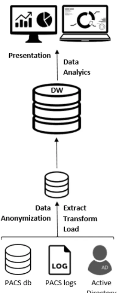
The system’s architecture, illustrated in figure3.1, is based on the main BI architecture2.2, where three main stages can be identified: Extract, Transform and Load (ETL); Data Analytics; Pre-sentation. The first one is where data extraction, data cleansing, data process and data migration to the main DW occurs. Although data anonymization is represented apart from ETL, it occurs within the ETL process. Then, clustering and association rules mining take place in data analytic stage. Finally, data is presented to the final users through interactive graphs, dashboards and other relevant formats.

3.2 Data Sources

Initially there was the need to identify what data and which data sources were going to be targeted. After discussing what data was required with the stakeholders, we established that data regarding medical staff, medical examinations and accesses to medical exams was needed to accomplish the goals of this dissertation. Such data is represented in table3.1.

Regarding medical staff data, we discard any personal information (e.g. name, age, sex, ad-dress) and only focus on the professional’s unique identifier, his/hers respective groups in the hos-pital’s domain and his/hers respective medical service (or medical specialty), that will be extracted from the domain groups. As to examinations, information regarding the type of examination (e.g.

(48)

Business Intelligence Solution Outline

Figure 3.1: Proposed BI system architecture

Thorax CT Scan), the medical imaging modality (e.g. CT), the body part of the exam (e.g. Tho-rax), if it has a report and its date, the examination’s date and the module of the exam (e.g. URG refers to emergency). Finally, concerning accesses to the exams we target who accesses the exam-ination - physician ID -, the action type (access or modify), the examexam-ination accession number and when the exam was accessed - access date. The accession number is the ID of the examination, so we will call it exam ID.

Since working under the General Data Protection Regulation (vide section2.3), we identify two fields that need to be encrypted: medical staff ID and exam’s accession number.

PACS has its associated software to visualize medical imaging, so information relative to ac-cesses to medical images are stored in logs. From there we can extract information regarding who accesses the exam, what exam is accessed and when the access occurs. Subsequently the data sources for this work were defined:

• Active Directory (AD): extract medical staff data.

• PACS database: extract information regarding the examinations; • PACS logs: extract information regarding accesses to the examinations.

(49)

Medical staff Examinations Accesses to exams ID Accession Number (ID) Medical staff ID Active Directory Groups Exam Code Action Type

Medical Specialty Modality Exam Accession Number Body Part Access Date

Body Description Report

Report Date Exam Date Module

Table 3.1: Required data for extraction.

3.3 Data Extraction, Transformation and Load

After properly defining what data was needed and where such data was stored, two scripts were made to extract the desired data. Since the whole process of data extraction was made on the client-side, there were many limitations regarding the technologies to be used.

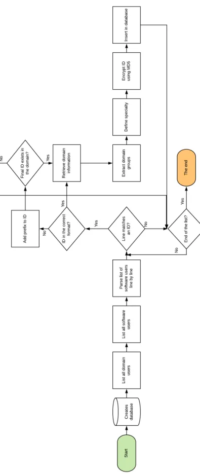
The first script was written using PowerShell1to extract information from the active directory. Powershell is the main scripting language used at Sectra due to the constraints previously men-tioned, and due to its versatility of the administration of applications that run on Windows Server environment and of its commands - cmdlets2. This script consists on matching the Sectra’s soft-ware users with the domain users and extract data - AD groups and the respective medical service. The information will be then stored in a sqlite3 database3.

As shown in the flow chart 3.2, the script first creates the proper database table with the re-quired fields - medical staff ID, domain groups and service -, then lists all the users in the software, with a specific command, that is not allowed to be revealed due to privacy agreements, and lists the domain users with the command net user /domain. We will go through each line in the listed software users and match each line referring to a user’s ID with the regular expression (?<=login: )(.*?)(?=$). The users in Sectra’s software may or may not directly match a user in the domain, since in the hospitals’ domain there is a certain prefix aggregated to the medical staff ID. When-ever there is no direct match between those two users, a certain prefix is added to the ID - final ID. Users may appear in both formats, resulting in replication of users. So for each user’s ID matched in the users software list, this verification will occur and the final ID will be matched with the listed domain users. If the final ID exists in the domain, then information regarding that user will be retrieved with the command net user <finalID> /domain and a regular expression is used to obtain the domain groups ((? <= Global Group memberships)([\s\S]∗)(? = T he command)). Fi-nally, the medical service is obtained from the domain groups, the final ID is encrypted in MD54 and those three fields are inserted in the sqlite3 database.

1_{https://docs.microsoft.com/en-us/powershell/scripting/overview?view=powershell-3.0} 2_{https://docs.microsoft.com/en-us/powershell/developer/cmdlet/cmdlet-overview}

3_{https://social.technet.microsoft.com/wiki/contents/articles/30562.powershell-accessing-sqlite-databases.aspx} 4_{https://en.wikipedia.org/wiki/MD5}

(50)

(51)

In its turn, the second script extracts the information relative to accesses by parsing the logs and extracts exams’ information by accessing the PACS database. To achieve such goal a script was written in Python 2.75 and several modules and libraries were used to parse XML files (Minimal DOM6), to connect to SQL server (pyobdc7), to encrypt (hashlib8) and to connect to the sqlite3. In order to overcome the impossibility of running Python scripts directly on the client-side, cx-freeze9 was also used for freezing the Python script into an executable, allowing this way the execution of the script on the client-side.

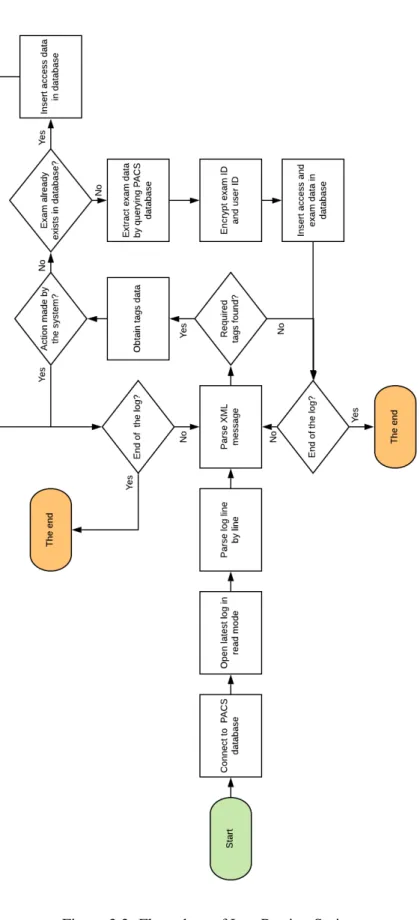
The script was ran everyday when the hospital has less activity between 1 a.m. and 6 a.m. -to avoid any potential conflicts and it parses the log of the previous day. The log is composed of XML messages, each message referencing a single action by a specific user or by the system.

As shown in the flow chart3.3, first the script connects to the SQL Server of the PACS database and then reads the last created log (the log of the previous day) and starts parsing the log. Different XML messages have different tags; since as we are only focusing on accesses to the exams, we look for specifics tags. Every XML message that does not have the required tags is discarded. For every XML message that matters, we extract data regarding the access - user (physician) ID, action type, access date, exam ID - and two verifications are done: if the user ID tag is referring to the system (occurs when a exam is created); if the exam ID already exists in our database. In the first case the XML message is discarded and the log parsing continues. In the second case since we already have the data regarding that exam, we only encrypt the user ID using MD5 and insert information regarding the access to the exam in the database. When none of these cases verify, we use the exam ID to query the PACS database and collect exam data (vide table 3.1). Then we encrypt both exam ID and user ID using MD5 and insert access data and exam data in the respective sqlite3 database. The program ends when we reach the end of the log.

After gathering all the necessary data, the sqlite3 database on the client-side was migrated to a PostgreSQL10 in our local machine. The final schema consists of three tables, similar to the table3.1(vide table3.2).

3.4 Preliminary Data Analysis

3.4.1 Research Variables

The research data set is composed by 442 158 objects which are characterised by 12 variables. Each object consists on a specific access, made by a health professional - exclusively physicians - to a medical examination. The research variables reference not only accesses, but also the ex-aminations and the health professionals. We were able to identify the medical service of 4804 doctors, and gather data in a 112 day period. The data set also corresponds to the medical exams

5_{https://docs.python.org/2/} 6_{https://docs.python.org/2/library/xml.dom.minidom.html} 7_{https://pypi.org/project/pyodbc/} 8_{https://docs.python.org/2/library/hashlib.html} 9_{https://cx-freeze.readthedocs.io/en/latest/index.html} 10_{https://www.postgresql.org/about/}

(52)

(53)

ADgroups examInfo auditInfo

pacsUserLogin (PK) accessionNr (PK) pacsUserLogin (FK)

groupName examCode actionType

service modality accessionNr (FK)

bodyPart accessDate bodyDescription report reportDate examDate module

Table 3.2: Final schema of the data extracted.

performed in the first 101 days, giving a 11-day window to only gather its respective accesses. Each object is characterized by two subsets of variables that describe: (1) the access; (2) the exam that is accessed.

1. Variables regarding the access:

• Physician ID: consists on a unique 32 digit hash that identifies a health professional. • Health Professional Service: indicates the service that the health professional is

as-signed. It is a categorical variable with 92 categories (vide appendixA.1).

• Date of access: indicates the date when the access occurs, in the format MM/D-D/YYYY. The date, in this study, can be between January 11 of the current year (01/11/2019) and May 2 (02/05/2019).

• Access Interval: indicates the time interval of when the access to the exam occurs, starting from the date when the exam is done. It is a categorical variable with 6 cat-egories: within the first week, within the second week, within the first month, within the second month, within the third month, within the forth month. For instance, if an examination is done on January 10 and the access occurs on January 15, we consider that the access occurs within the first week. If the access occurs on January 25, we consider that the access occurs within the first month. These categories are mutual exclusive. That means we only consider an access within the second month when the access happens after 30 days, from the exam date, and before 60 days.

2. Variables regarding the exam:

• Exam accession number: consists on a unique 32 digit hash that identifies an exam. • Exam date: indicates the date when the exam is done, in the format MM/DD/YYYY.

In this study, it ranges from 01/11/2019 to 04/21/2019.

• Exam code: consists on a number that specifies the type of exam. There are 758 different exam codes.

Analysis of Usage Patterns of Medical Image Exams in Medical Environments

F

E

U

P

Analysis of usage patterns of medical

image exams in medical environments

Nuno Martins Marques Pinto

Analysis of usage patterns of medical image exams in

medical environments

Nuno Martins Marques Pinto

Mestrado Integrado em Engenharia Informática e Computação

Approved in oral examination by the committee:

Abstract

Resumo

Acknowledgements

Contents

List of Figures

List of Tables

Abbreviations

Chapter 1

Introduction

1.1

Context and Problem

1.2

Motivation and Objectives

1.3

Dissertation Structure

Chapter 2

Background Knowledge

2.1

Health Information Systems

2.2

Business Intelligence

∑

∑

∑

∑

∑

∑

2.3

Data Anonymization

2.4

Related Works

Chapter 3

Business Intelligence Solution Outline

3.1

Overview

3.2

Data Sources

3.3

Data Extraction, Transformation and Load

3.4

Preliminary Data Analysis