Facades and solar parking yield estimation at Ultrecht University

Mestrado em Engenharia da Energia Solar

Relat´orio de Est´agio

Facades and solar parking yield estimation at Utrecht

University

T´

ayzer Damasceno de Oliveira

Orientador(es) | Lu´ıs Fialho Atse Louwen

Wilfried G.J.H.M. van Sark

´

Relat´orio de Est´agio

Facades and solar parking yield estimation at Utrecht

University

T´

ayzer Damasceno de Oliveira

Orientador(es) | Lu´ıs Fialho Atse Louwen

Wilfried G.J.H.M. van Sark

´

• Presidente | Paulo Canhoto (Universidade de ´Evora)

• Vogal | Fernando Manuel Tim Tim Janeiro (Universidade de ´Evora) • Vogal-orientador | Lu´ıs Fialho (Universidade de ´Evora)

´

Dedico este trabalho à minha família que sempre me apoiou. Ao Prof. Luis Fialho pela orientação e toda ajuda que providenciu neste trabalho. Ao Prof. Wilfried, Dr. Atse, Msc. Nick and Msc. Marte por toda ajuda com meu projeto durante minha estadia de Erasmus na Universidade de Utrecht. E a todos os meus amigos que estiveram comigo durante essa jornada.

ASTRACT

Solar energy born as one of the ways to produce energy using renewable resources (like wind, biomass, hydraulic, geothermal and wave energies). The solar energy is divided into three types: thermal, that generates heat (which can be used to produce energy), photovoltaic that only produces electricity and PVT, a hybrid way to generate heat and produce electricity. Photovoltaic (PV) technologies have several uses such as lighting, satellites, solar home systems, pumping, etc. This work pretends to estimate the potential of usage of solar cells and the yield potential at De Uithof campus located in Utrecht, Netherlands. Building attached photovoltaic (BAPV), solar parking lot and charging electric vehicles (EV) were the chosen uses of solar energy for this project. The work method is divided into four parts, firstly a 2D part that was done on ArcGIS software to create the shapefile with the buildings and solar parking information of the incoming radiation for the entire year in Wh/m2_{. Secondly, the 3D works on}

AutoCAD, Autodesk FBX Converter and PVsyst to create the 3D plant and to import the shading scene construction, to install the solar modules on the roofs, facades and solar parking lot. The third part is to choose the charging mode 3 combined with connector type 2 that full charge the Tesla model 3 (which has a battery of 50 kWh) in around five hours (charging 11kW per hour). The fourth part details the input data and calculate the economic viability considering the total cost of initial investment and operation/maintenance costs. Two tests were used to compare different options, VC0 (35.175 kWp) with the solar modules facing south and VC1 (50.796 kWp) on the west-east plus south direction. The chosen PV module was the LG 340 N1C-A5 by LG Electronics and the inverter was the AGILO 100.0-3 Outdoor by Fronius International because they are commercially available equipments. The VC0 has a system production of 27.229 MWh/year and the VC1, 35.285 MWh/year, both are feasible economically because they have the NPV greater than zero, being €68 million for VC0 and €83 million for VC1. In addition, the Payback is much lower than 25 years (lifetime of photovoltaic panels), being 7,69 years and 7,03 years, respectively for VC0 and VC1. Furthermore, the LCOE of the VC0 is 0.058 €/kWh, and for VC1, 0,064 €/kWh.

A energia solar surgiu como uma das diversas maneiras para produzir energia elétrica utilizando recursos renováveis (como a energia eólica, biomassa, hidráulica, geotérmica e das ondas). A energia solar é dividida em três tipos: térmica, que gera calor (que também pode ser usado para produzir energia), fotovoltaica que somente produz eletricidade e PVT, maneira híbrida de gerar calor e produzir eletricidade. Tecnologia fotovoltaica tem diversos usos como iluminação, satélite, sistemas solares residenciais, bombeamento, entre outros. Este trabalho pretende estimar o potencial do uso de células solares e a potência anual no campus De Uithof que se localiza em Utrecht, Países Baixos. Building attached photovoltaic (BAPV), estacionamento solar e carregamento de veículos elétricos (EV) foram os usos da energia escolhidos para este projeto. O método do trabalho se divide em quarto partes, primeiramente a parte 2D que foi feita no software ArcGIS para criar shapefile com as informações da radiação que chega aos prédios e estacionamento durante todo o ano em Wh/m2_{. Segundamente, o 3D}

feito no AutoCAD, Autodesk FBX Converter e PVsyst para criar a planta 3D e importar no Shading scene construction, instalar os módulos solares nos telhados, fachadas e estacionamento solar. A terceira parte foi escolher o modo de carregamento 3 combinado com o conector 2 que carrega completamente o Tesla model 3 (possuindo bateria de 50 kWh) em aproximadamente em cinco horas (carregando 11 kW por hora).A quarta parte detalha os dados de entrada e calcula a viabilidade econômica considerando o custo total de investimento e custos de operação/manutenção. Dois testes foram feitos de modo a compará-los, VC0 (35.175 kWp) com os módulos solares virados para sul e VC1 (50.796 kWp) nas direções este-oeste e direção sul. O painel escolhido foi o LG 340 N1C-A5 da LG Electronics e o inversor AGILO 100.0-3 Outdoor da Fronius International porque são equipamentos comerciais. A produção do VC0 é de 27.229 MWh/ano e o VC1, 36.614 MWh/ano, os dois são economicamente viáveis porque possuem o VPL (NPV) maior que zero, sendo €68 millhões para o VC0 e €83 para o VC1. Adicionalmente, o Payback possui um valor bem abaixo de 25 anos (ciclo de vida dos paineis fotovoltaicos), sendo 7,69 anos e 7,03, respectivamente VC0 e VC1. Além do mais, o LCOE do VC0 é 0.058 € /kWh, e para o VC1, 0.064 €/kWh.

Summary

1. Introduction ... 13

1.1. Objective ... 13

1.2. Thesis Structure ... 14

2. State of the art ... 15

2.1. Solar energy technologies ... 15

2.1.1. Photovoltaic ... 15

2.2. Solar parking lot ... 19

2.2.1. Rigid cover system ... 19

2.2.2. Flexible cover system ... 20

2.3. Building Attached Photovoltaic (BAPV) ... 21

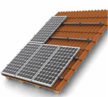
2.3.1. Tile-on roof system ... 21

2.3.2. Metal sheet roof system ... 22

2.3.3. Flat roof system ... 23

2.4. Charging technologies ... 23

3. Method ... 25

3.1. 2D part ... 26

3.1.1. Datasets – take the raster from AHN website ... 26

3.1.2. Make the shapefile using ArcGIS ... 27

3.1.3. Tool “Area Solar Radiation.” ... 30

3.2. 3D part ... 31

3.2.1. Export the Shapefile of the buildings to AutoCAD to do the extrusion ... 31

3.2.2. Import this file on PVsyst; ... 32

3.2.3. Input data on PVsyst; ... 32

3.3. Carbon balance calculus ... 35

3.4. Charging stations ... 36

3.5. Economic analysis for the PV project ... 38

4. Results ... 43

4.1. Solar potential ... 43

4.1.1. 2D results ... 43

4.1.2. 3D results ... 44

4.1.3. Carbon balance result ... 47

4.2. EV Charging ... 48

4.3. Economic analysis ... 55

Figures

Figure 1 - Mono-crystalline cell and module ... 16

Figure 2 - Poly-crystalline cell and module1 _{... 16}

Figure 3 - Amorphous solar cells1 _{... 17}

Figure 4 - Cadmium-Telluride solar cell ... 18

Figure 5 - Copper-Indium-Gallium-Selenide solar cell2 _{... 18}

Figure 6 - Organic solar cell1 _{... 19}

Figure 7 - Car Schell Energy, GREENPARK ... 20

Figure 8 - SmartPark solution – Martifer solar3 _{... 20}

Figure 9 - Skyshade solution3 _{... 21}

Figure 10 - Hightex solution3 _{... 21}

Figure 11 - Tile-on roof system ... 22

Figure 12 – Metal sheet roof system4 _{... 22}

Figure 13 - Flat roof system4 _{... 23}

Figure 14 – Method organogram ... 25

Figure 15 - De Uithof ... 26

Figure 16 - Height with reference at sea level (m) ... 27

Figure 17 - Maximum height of buildings (m)7 _{... 28}

Figure 18 - Shape area of the buildings (m2₎7 _{... 29}

Figure 19 - Solar parking area (black squares)7 _{... 30}

Figure 20 – Buildings and solar parking view from the top ... 31

Figure 21 - Location of weather station ... 32

Figure 22 – Facades tilt and azimuth angles for both projects ... 33

Figure 23 -Tilt and azimuth angles for VC0 used in solar parking and roofs ... 33

Figure 24 – Tilt and azimuth angles for VC1 used in solar parking and roofs for West direction ... 33

Figure 25 - Tilt and azimuth angles for VC1 used in solar parking and roofs for East direction ... 33

Figure 26 - VC0 project9 _{... 34}

Figure 27 - VC1 project9 _{... 35}

Figure 28 - Tesla Model 3 ... 36

Figure 29 - Type 2 (Mennekes - IEC 62196)10 _{... 36}

Figure 30 - Radiation for the entire year (Wh/m2) ... 44

Figure 31 - Carbon balance for VC09 _{... 47}

Figure 32 - Carbon balance for VC19 _{... 48}

Graphics

Graphic 2 - Monthly Average vs Time for VC1 ... 50

Graphic 3 - Number of charging stations for entire project vs time for VC0 ... 51

Graphic 4 - Number of charging stations for entire project vs time for VC1 ... 52

Graphic 6 - Number of charging stations for solar parking vs time for VC1 ... 54

Graphic 7 - Accumulated cash flow for VC0 and VC1 ... 56

Tables

Table 2 – Connectors type using IEC 62196-2 standars5 _{... 24}

Table 3 - Modes of charging using connector Type 210 _{... 37}

Table 4 - CAPEX for VC0 ... 41

Table 5 - CAPEX for VC1 ... 41

Table 6 - Results overview ... 45

Table 7 - System information ... 45

Table 8 - Balances and main results of VC0 ... 46

Table 9 - Balances and main results for VC1 ... 47

Table 10 - Average number of charged cars per day ... 55

Table 11 - Output data for VC0 ... 55

CIS - Copper-Indium-Selenide

CIGS - Copper-Indium-Gallium-Selenide CPV – Concentrated photovoltaic

BIPV – Building integrated photovoltaic BAPV – Building attached photovoltaic BiPVT/a - building-integrated installations BiPVT/w - Building-integration installations EV – Electric vehicles

GHG – Greenhouse gases CAPEX – Capital expenditure OPEX – Operational expenditure NPV – Net present value

IRR – Internal rate return TLCC – Total life-cycle cost LCOE – Levelized cost of energy PVC - Polyvinyl chloride

PTFE – Polytetrafluoroethylene

EVSE - Electric vehicle supply equipment IEC - International Electrotechnical Commission AC - Alternating Current

DC - Direct Current

PDOK - Public Services On the Map AHN - Actueel Hoogtebestand Nederland LCE - Life cycle emission

Pnom - Nominal power

GlobHor - Horizontal global irradiation DiffHor - Horizontal diffuse irradiation T_amb - Ambient temperature

GlobEff = Effective global IAM (Incidence Angle Modifier Earray = Effective energy

E_Grid = Energy injected into the grid PR = Performance ratio

1. Introduction

The use of renewable energies is one of the ways for reducing the emission of greenhouse gases, furthermore we do have several sorts of energies that use renewable sources like wind (wind energy), earth heat (geothermal), water (hydropower), sun (solar energy) and wave/tidal (tidal energy).

There are three possibilities for using the solar energy, solar thermal (heat only, which can, in turn, be used to generate electricity), photovoltaic (electricity only) and PVT (heat and electricity).

For solar thermal energy, can be divided into active and passive solar system. Active system is the solar collectors like flat-plate collectors and concentrated solar power systems (compound parabolic collectors, heliostat field collectors, linear fresnel collectors, parabolic dish reflectors, and more). In another side, passive solar system does not have the reliance on external devices, can be used for cooling and heating for sunroom, greenhouse, solariums (Tian, 2013).

Photovoltaic solar energy is used for generating energy but with different PV technologies, based on the commonly characteristics, splits in four majors: Crystalline silicon (Mono or Poli), Thin film (Amorphous, CdTe, CIS, CIGS), Organic and Concentrated photovoltaic (CPV). Furthermore, has several sorts of uses, such as lighting; satellites; solar home systems; pumping; integrated (BIPV) or attached (BAPV) in buildings; charging vehicles/bikes/etc; solar parking; desalination plant; isolated system; etc (Eldin, 2015).

For PVT, we have a hybrid system with photovoltaic and thermal, that have three collector types that are flat plate PVT collectors, concentrating PVT collectors and water and air type PV/T collectors, can be used at building-integrated installations (BiPVT/a), Building-integration installations (BiPVT/w), and more (Charalambous, 2007; Chow, 2010).

1.1. Objective

As the use of solar energy is growing every year, many countries are increasing the use of solar energy on the energy mix. Netherlands, in 2017, added 853MW on the solar power system (Netherlands, 2018), this information shows that the country cares about the gas pollution that happens using fossil fuel to produce energy, and the context takes us to use the solar energy on the commercial/residential buildings and also inside the University demonstrating to the students the importance of using renewable energies (solar energy on this project) and how it works.

At Uithof campus, there are several options for using solar energy, this project focus on BAPV, solar parking and EV charging. The reason to use the BAPV is that the buildings are in use, so this might be cheaper to attach rather than change the structure to integrate the solar panels on the buildings (BIPV). Solar parking is a good way to produce energy using the parking lot spaces, besides protecting them from the meteorological conditions. In addition, choose EV to reduce GHG emission.

The goal for this project is to estimate the yearly yield potential (PVsyst uses a stochastic algorithm that calculates hourly data, using generic data and unspecific year) using solar panels inside the De Uithof campus located at Utrecht, Netherlands which contains the Utrecht Science Park, the campus area of Utrecht University, the vocational University Hogeschool Utrecht and the academic hospital University Medical Center Utrecht (UMCU). Building attached photovoltaic (for the roofs and facades), solar parking lot and charging vehicles are the chosen uses of solar energy for the present project.

Two layouts (VC0 and VC1) are used in this project to compare energy production, first with the modules on the south direction (Azimuth 0°), the second with west-east direction (Azimuth -90° and

The following lead question for this thesis is: is economically feasible to install solar panels around the Uithof campus and provide energy to charge EV through the charging station?

Using the software ArcGIS, AutoCAD and Pvsyst are possible to construct the entire project that answer: It is possible to use the solar photovoltaic energy around the campus?

Simulating the yield potential, and doing a calculus using the produced energy with the charging station and connectors can be possible to answer the question: Could we use the power electricity for charging EV?

Estimate the CAPEX, OPEX, taxes, to evaluate the NPV, Payback, IRR and LCOE that answer: Is it economic feasible to install this power system?

1.2. Thesis Structure

Section 2 presents the state of the art for photovoltaic technology, solar parking lot (rigid or flexible cover system with the solar panels integrated or attached), building attached photovoltaic (solar panels with metallic support on the roofs and facades) and charging technologies (different levels of charging).

Section 3 describes the method, which contains the step by step to get the result. Firstly, the 2D part consists of using the ArcGIS to make the shapefile of the building/solar parking on the De Uithof campus which shows the solar radiation for the entire year. Then doing the 3D on the AutoCAD with the extrusion using the maximum height of the buildings, plus using the PVsyst to attach the solar panels on the roofs, facades and solar parking that allows the yearly yield simulation that includes the shading and losses. Carbon balance calculus that represents the amount of dioxide carbon emission that will be avoided. The fourth part displays the EV (electric vehicle) and the type of charge used on this work. In sequence, the input data for a short economic analysis.

Section 4 displays the results that splits into three categories: Solar potential, that includes the 2D part, 3D part and Carbon balance; EV charging, which has a rough calculation for the numbers of cars loaded per day and the quantity of charging stations that can work simultaneously; Economical analysis, displays the values for NPV, IRR, Payback, TLCC and LCOE.

Section 5 has a conclusion about the project showing some results. Section 6 illustrates the future works that describe the next steps to get better results with more accuracy.

2. State of the art

Presently, solar energy has several sorts of use, and three of them are going to be used on this work, the chosen sorts are solar parking (Section 2.2), building attached photovoltaic (Section 2.3) and charging electric vehicles (Section 2.4).

2.1. Solar energy technologies

Solar energy is the radiant light and heat that comes from the Sun capable of producing heat, chemical reactions or generating electricity. For generating electricity, there is the photovoltaic technology that consists of a PV cell containing a semiconductor device that converts solar energy into direct-current electricity (Ellabban, 2014).

2.1.1. Photovoltaic

Used for generating energy but with different PV technologies, based on the common characteristics, splits among three majors: Crystalline silicon (Mono or Poly), Thin-film (Amorphous, CdTe, CIS, CIGS) and Organic.

• Crystalline silicon (Mono or Poly)

The first generation of solar cells uses Silicon that is a semiconductor material, with an energy band gap of 1.1 eV. Is the most common PV technology use in the PV industry and have constant development. There are two types of crystalline silicon that depend on the structure of the crystals, mono- and poly- crystalline (Eldin, 2015).

o Monocrystalline (m-Si)

The Monocrystalline Silicon cells (Figure 1) is the type of PV technology most commonly used, these cells are obtained from cylindric bars made by mono-crystalline silicon that is produced in a special oven. Those bars are cut into thin slices (wafers), with a thickness of around 200 µm with the efficiency reaching up 20% (Eldin, 2015).

Figure 1 - Mono-crystalline cell and module1

o Polycrystalline (p-Si)

The Polycrystalline (Figure 2) are produced from the fusion of silicon blocks, in other words, the process to junction the silicon crystals, that reduces the efficiency compared with the mono-crystalline, with the value reaching 15% (El Chaar, 2011).

Figure 2 - Poly-crystalline cell and module1

• Thin film (Amorphous, CdTe, CIS, CIGS)

With the expensive process for producing solar cells based in crystalline cells, the manufacturing of thin films is a cheaper alternative, i.e., lower manufacturing cost. In addition, this kind of solar cells can be so flexible and lightweight, so has the possibility to be easily installed in BIPV, BAPV, etc (Eldin, 2015). The classify of thin films depends on the substance on the solar cell, existing three types:

o Amorphous Silicon (a-Si)

Amorphous technology (Figure 3), if we compare with the crystalline silicon, the atoms are randomly located from each other, this property makes the band-gad being higher (1.7 eV) than crystalline silicon (1.1 eV) (El Chaar, 2011). Have lower efficiency (range between 4% to 8%) but do not use toxic heavy metals such as Cadmium or Lead.

Figure 3 - Amorphous solar cells1

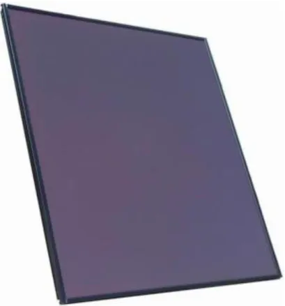
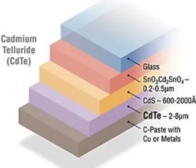
o Cadmium-Telluride (CdTe)

The big disadvantage of CdTe solar cell (Figure 4) technology is the fact of having Cadmium which is a heavy metal and toxic for the environment, despite the fact that has the ideal band-gap (1.45 eV) with high direct absorption coefficient, the efficiency can reach 15% (El Chaar, 2011).

Figure 4 - Cadmium-Telluride solar cell2

o Copper-Indium-Selenide (CIS) and Copper-Indium-Gallium-Selenide (CIGS)

CIS cells are made using a thin layer of CuInSe2 with band-gap 1.04 eV and the CIGS (Figure

5), a thin layer of Cu(In,Ga)2Se2 with band-gap 1.68 eV. The efficiency is the biggest advantage cause

can reach 20% with solar cells having 0.5 cm2 _{(El Chaar, 2011).}

Figure 5 - Copper-Indium-Gallium-Selenide solar cell2

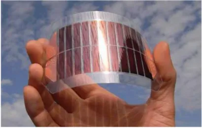
• Organic

Organic solar cells (Figure 6) are composed using organic or polymer materials, the manufacturing cost is cheap but unfortunately, this kind of cells are not very efficient. With the possibility to use plastic sheets as a coating that makes the organic solar cells lightweight and flexible (Eldin, 2015).

Figure 6 - Organic solar cell1

Applications for PV are Building integrated/attached systems (BIPV and BAPV), desalination plant, space, solar home systems, communications, rural electrification, lighting, reverse osmosis plants, pumps, photovoltaic and thermal (PVT) collector technology and others (PARIDA,2011).

2.2. Solar parking lot

The solar parking lot is the possibility of using the PV panels on the roof of the parking lots, sometimes is possible to build the roof using the solar panels rather than attaching the PV panels. This solution is good for charging electric bikes and cars, and possibly electronic equipment (notebooks, cell phones, power banks, etc). This technology is good to protect bikes and cars from meteorological conditions like sun, rain, snow, wind, and hail.

Basically, we have two types of parking lot cover systems that are the most used: rigid cover system and flexible cover system. The rigid system is most used, but both may have a different aesthetic structure.

Correia (2013) presents on their study both types of cover system, beyond showing the possibility to use the PV panels on the parking structures and the different aesthetic structures that were made by some companies.

2.2.1. Rigid cover system

Rigid system is the traditional solution, usually made of steel which has some advantages like the lowest price, fast execution, and maximum use of space with the possibility to do different structures. To avoid corrosion problems, galvanized and stainless steel are used. Other materials can be used for the parking structures like aluminium, glass panels, polymer panels or PVC covers. Figure 7 and Figure 8 displays examples made by two companies using integrated solar parking.

Figure 7 - Car Schell Energy, GREENPARK3

Figure 8 - SmartPark solution – Martifer solar3

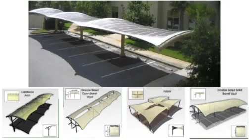
2.2.2. Flexible cover system

Flexible cover system has metal support for the tensile membrane cover. When adopting this solution, the advantage is a having lightweight roof, fewer numbers of pillars and structural steel, with the possibility to use the PVC, PTFE, glass fiber and silicon. Figure 9 and Figure 10 shows two designs for a membrane cover system with solar panels.

Figure 9 - Skyshade solution3

Figure 10 - Hightex solution3

2.3. Building Attached Photovoltaic (BAPV)

BAPV are added on rather than integrated into the roof or facade, for this option, any PV technology can be used as needs small metal support to fix the PV panels.

2.3.1. Tile-on roof system

This type is used at tile roofs like hollow, flat roof, standard, double slot, roman, plain, scale, bitumen, slate and spanish tiles, the PV modules are fixed on the roof using hooks and mounted using rails and clamps. Figure 11 shows one of the examples of the tile-on roof system.

Figure 11 - Tile-on roof system4

2.3.2. Metal sheet roof system

This type of system is used in metal sheet roof is considerate hardcore for roof system, but with matched clamp and rail is possible to fix the PV panels on the metal sheet roofs. Figure 12 displays an example.

Figure 12 – Metal sheet roof system4

2.3.3. Flat roof system

Flat roof system can be used in all kind of flat roofs according to the roof support capacity with the weight of the solar plant and waterproof requirements. Figure 13 illustrates one of the examples that uses concrete (or other material) blocks or chemical anchor bolt to fix the system on the roof.

Figure 13 - Flat roof system4

2.4. Charging technologies

To charge your electric vehicle (EV) requires plugging into charger equipment that is connected on the electric grid, and the equipment calls electric vehicle supply equipment (EVSE) (Morrow, 2008). There are four models of charging that depends on the amount of power comes from the charger to the battery, furthermore, four connector types. Table 1 shows the charging modes following the IEC-61851-1 standard.

Table 1 - Charging modes using IEC-61851-1 standard5

Mode

Specific connector for

EV

Type of charge Maximum current Protections

Mode 1 No Slow in AC 16 A per phase (3,7 kW - 11

kW)

The installation requires earth leakage and circuit

breaker protection

Mode 2 No Slow in AC 32 A per phase (3,7 kW - 22

kW)

The installation requires earth leakage and circuit

breaker protection

Mode 3 Yes

Slow or semi-quick, Single-phase or

three-phase

In accordance with the connector used

Included in the special infrastructure for EV

Mode 4 Yes In DC In accordance with the charger Installed in the

infrastructure

Table 2 shows the connectors type following the IEC 62196-2 standard.

Type 2 7 (L1, L2, L3, N, PE, CP, PP) 500 V a.c. Three-phase, 250 V a.c. Single-phase 63 A three-phase (up to 43 kW), 70 A single-phase Type 3 4, 5 or 7 in accordance with the model (L1, L2,

L3, N, PE, CP, PP) 500 V a.c. Three-phase, 250 V a.c. Single-phase 16 / 32 A single-phase, 32 A three-phase (up to 22 kW)

3. Method

Section 3 begins with the selection of the location where the PV system will be installed. On Section 3.1, the 2D (only ArcGIS) details the steps to create the buildings/solar parking lot shapefile. The 3D (AutoCAD and PVsyst) is described on Section 3.2 featuring the extrusion on AutoCAD to build the objects in 3D, importing the file on PVsyst and projecting the system inserting input data to simulate the yearly yield potential. Section 3.3 details the dioxide carbon balance calculus. Section 3.4 displays the calculus for estimating the quantity of charging stations working simultaneously and the number of cars that can be charged at the same time. Section 3.5 attributes the input data for economic viability and the variables that will be calculated. Figure 14 displays briefly the step by step to get the result.

Figure 14 – Method organogram

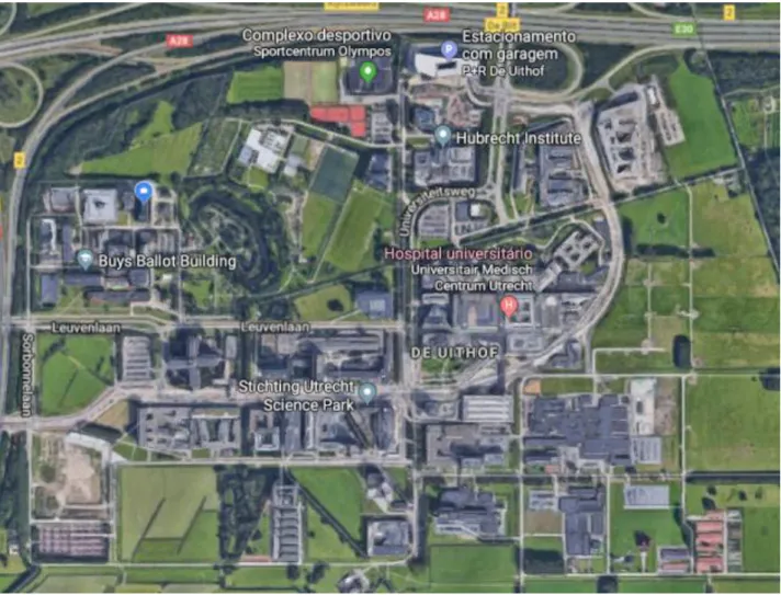
Firstly, the location for the project needs to be chosen, so for the present project, the De Uithof campus located at Utrecht, Netherlands was selected (Figure 15).

2D

•Take the raster file from AHN website

•Make the shapefiles (having the buildings and solar parking) using ArcGIS

3D

•Export the shapefile to AutoCAD

•Extrusion on the AutoCAD with the maximum height of the buildings

•Export the CAD file to import at PVsyst

•Input data at PVsyst (module, inverter, 3D scheme, design and more)

•Simulation

Calculations

•Carbon Balance Calculus •Charging station •Economic viability for PV

system

Results

Figure 15 - De Uithof 6

3.1. 2D part

3.1.1. Datasets – take the raster from AHN website

To import the raster files on ArcGIS, the .DSM raster file (intended as a raw file, with all points except those classified as "water" being resampled to a grid based on a Squared IDW method. No further operations have been performed) can be found at PDOK (Public Services On the Map) website (AHN, 2019). The files 31HZ2 and 32CZ1 are chosen to be cut and merge using the ArcGIS which is Figure 16. The values show the maximum height considering the sea level as a reference that starts from -1 m (because some parts of Netherlands are below the sea level) reaching to 92 m (tallest building).

Figure 16 - Height with reference at sea level (m)7

3.1.2. Make the shapefile using ArcGIS

Meuser (2018) provides a shapefile showing the entire Netherlands, so was possible to cut the De Uithof campus. Figure 17 and Figure 18 show the De Uithof campus shapefiles focusing on the buildings.

Figure 17 exhibits the maximum height of the buildings that subdivide into five levels ranging from 4,97 m to 87,87 m.

Figure 17 - Maximum height of buildings (m)7

Figure 18 illustrates the shape area (in m2_{) that represents the geometry area of the buildings.}

The shape area of the buildings has five levels that go from 31,43 m2 _{to 61.335,31 m}2_.

Figure 18 - Shape area of the buildings (m2₎7

Figure 19 displays the solar parking places (in black), around the campus there is a possibility to install more solar parking lots, but they are not suitable because they are shaded from the buildings or trees.

Figure 19 - Solar parking area (black squares)7

3.1.3. Tool “Area Solar Radiation.”

“The Area Solar Radiation tool is used to calculate the insolation across an entire landscape. The calculations are repeated for each location in the input topographic surface, producing insolation maps for an entire geographic area” (Area, 2019), in other words, this tool provide the total amount of incoming solar insolation (direct + diffuse) for the entire year for each location in Wh/m2_.

3.2. 3D part

For the 3D, Pvsyst was chosen because is possible to do a three-dimensional project that uses the horizon limitations and objects that produce shadows on the panels. There are four main options to design the project: the PV system as Grid-connected (connect to the grid with the option to use or not a battery), Standalone system, Pumping system or DC grid connected (connected into the grid without battery).

The software has an quite extent input data and allows to choose the PV modules (model, quantity, orientation, etc.), the inverter (model and quantity), number of subarrays (limit of eight subarrays), 3D scene (possibility to draw the PV system in 3D and to introduce the construction and/or elements that cause shadows). The output data has several result options such as yearly yield potential, performance ratio, carbon balance, and other options.

The advantages of using this software are the big database which contains several options of cities where the project can be installed; the modules and inverters available on the software are totally commercial; several parameter options for the panels setup such as fixed, one-axis, two-axis tracking, its subdivisions into arrays and strings; etc.

3.2.1. Export the Shapefile of the buildings to AutoCAD to do the

extrusion

Figure 20 displays the buildings (white lines) and solar parking (green line) top view.

Figure 20 – Buildings and solar parking view from the top8

3.2.3. Input data on PVsyst;

For the project, VC0 and VC1 (names provided on the software to the different projects) represent the simulation tests:

• VC0 – with the modules facing South - Azimuth of 0°, but some turned because of the facades or roofs of the buildings; 90° tilt for the facades and 34° tilt for the roofs and solar parking; • VC1 – with the panels facing South + West-East direction – Azimuth of 90° and -90°, the larger

number of modules with the West-East side orientation, but some stayed turned to the South, the Tilt angle is 90° for the facades and 34° for the roofs and solar parking.

On both projects, the entire solar power plant is split into three parts: solar parking, facades, and roofs.

❖ Site and Meteo – for the country and city where the project will be installed

Figure 21 specifies the information about the location of the nearest weather station of Utrecht, in the city called De Bilt. Its latitude is 52,10°N, longitude 5,18°E, time zone UT+1, the altitude of the weather station is 1 m and the albedo is 0,20.

Figure 21 - Location of weather station9

❖ Orientation

For both test setups (VC0 and VC1), the tilt is the same, 90° for the facades (Figure 22), and 34° for the roofs and solar parking (Figure 23 for VC0, Figure 24 and Figure 25 for VC1). The difference is in the Azimuth for the roofs and solar parking that on the VC0 are totally facing South (0° and some to other directions due the buildings orientation restrictions), the majority of the modules in VC1 is simulated with the West-East setup (90° and -90° for 100% in solar parking, the roofs have some

exceptions facing South, due to architecture limitations). The facades are the same for both projects (VC0 and VC1).

Figure 22 – Facades tilt and azimuth angles for both projects

Figure 23 -Tilt and azimuth angles for VC0 used in solar parking and roofs

Figure 24 – Tilt and azimuth angles for VC1 used in solar parking and roofs for West direction

(Figure A 2). The nominal PV power DC at 104 kW, maximum PV power DC at 150 kW. And the operating mode at MPPT (maximum power point tracking) with minimum and maximum voltage at N/A and 820 V, respectively.

❖ Detailed losses – Default options were used.

❖ Self-consumption - No auto-consumption was chosen.

❖ Storage – No storage was chosen.

❖ Near shading

With the Shading scene construction, it is possible to construct the entire project with the PV modules and the buildings (including the possibility of shading by the building and modules). Figure 26 illustrates the project VC0 with modules facing South. Figure 27 displays the project VC1 with the modules installed with the West-East direction plus South scheme.

Figure 27 - VC1 project9

3.3. Carbon balance calculus

Another valuable tool on PVsyst is the Carbon Balance estimation that represents how much the system will save regarding CO2 emissions. The calculus is based on the life cycle emission (LCE)

method, which represents the emissions of CO2 associated to a given component or energy amount,

including production, operation, maintenance, disposal, etc. (User’s, 2012). To estimate the Carbon Balance, Equation 1 shows its balance:

Equation 1

𝐵𝐶𝑎𝑟𝑏𝑜𝑛𝑜 = 𝐸𝐺𝑟𝑖𝑑𝑆𝐿𝑖𝑓𝑒𝑡𝑖𝑚𝑒𝐿𝐶𝐸𝐺𝑟𝑖𝑑− 𝐿𝐶𝐸𝑆𝑦𝑠𝑡𝑒𝑚

Where:

Bcarbon – Carbon balance (tCO2).

EGrid – Energy injected into the grid (MWh).

SLifetime – System Lifetime – Represents the lifetime of the PV installation (Year).

LCEGrid – Grid LCE - Represents the average amount of CO2 emissions per energy unit for the electricity

produced by the grid (Fix value for each country) (gCO2/kWh).

LCEsystem – PV system LCE – Represents the total amount of CO2 emissions caused by the construction

charging process, there are four different modes of charging (Section 2.4), for the present project and being a commercial usage, mode 3 combined with connector type 2 (accepted on Tesla Model 3 - Figure 29) are adopted as taking around 5 hours, Table 3 displays the different modes of charging using the Type 2 connector, using the charging point for 3-phrase 16A that charges 11kW per hour, the car will be full charge in around 5 hours that is the average time for work/study. The reason to choose Tesla Model 3 is that is one of the commercial brands for EV.

Figure 28 - Tesla Model 310

Figure 29 - Type 2 (Mennekes - IEC 62196)10

Table 3 - Modes of charging using connector Type 210

Charging Point Max. Power Power Time Rate

Wall Plug (2.3 kW) 230V / 1x10A 2.3 kW 23h45m 8 mph

1-phase 16A (3.7 kW) 230V / 1x16A 3.7 kW 14h45m 13 mph

1-phase 32A (7.4 kW) 230V / 1x32A 7.4 kW 7h30m 25 mph

3-phase 16A (11 kW) 400V / 3x16A 11 kW 5 hours 38 mph

3-phase 32A (22 kW) 400V / 3x16A 11 kW † 5 hours 38 mph

To estimate the number of charging stations working simultaneously for the entire project versus hourly time for the VC0, in other words, the number of cars being charged at the same time using 11 kWh to charge the EV, the calculus uses Equation 2.

Equation 2

𝑁𝑇 =

𝐸𝐺𝑟𝑖𝑑

𝐿𝐶 Where:

NT – Number of charging stations for the entire project

E_Grid – Hourly energy injected into the grid (kWh) LC – Capacity charged for each car (for example: 11 kWh)

To determine the number of charging stations working simultaneously for the solar parking versus hourly time for the VC0, this calculus uses the following Equation 3.

Equation 3

𝑁𝑆𝑃 = 𝑁𝑇 ∗ %𝑆𝑃

Where:

NSP – Number of charging stations for the solar parking

NT – Number of charging stations for the entire project

%SP – Percentage of the Solar Parking (Value of 6,23%)

To quantify the Average number of charged cars per day for the entire project and for the solar parking, Equation 4 and Equation 5, respectively, are used.

NCT – Number of charged cars for the entire project.

ƩE_Grid – Sum of the hourly energy injected into the grid (kWh). BNL – Tesla Model 3 battery capacity (50 kWh).

Equation 5

𝑁𝐶𝑆𝑃 = 𝑁𝐶𝑇∗ %𝑆𝑃

Where:

NCSP – Number of charged cars for the solar parking.

NCT – Number of charged cars for the entire project.

%SP – Percentage of the Solar Parking.

3.5. Economic analysis for the PV project

At this stage, the cash flow spreadsheet contains the initial investments (which represents the CAPEX) and the annual spending with operation and maintenance (OPEX). For this analysis, the parameters are:

• Initial investment: describes the expenses regarding the purchase of: value of the PV panels, inverters, structures (for roofs to use the top of the buildings to produce energy also decreasing the heat inside the building; facades, was not able to find a 90° degree structure; and solar parking, using the up part of the solar parking to produce energy, furthermore to charge EV or other electronic stuff) and labor cost (for installing the solar power plant);

• Annual spending: operation and maintenance.

For a simple economic analysis, four variables need to be calculated: The NPV (Net present value), TLCC (total life-cycle cost), Payback, IRR (Internal rate of return) and LCOE (Levelized cost of energy). The calculus uses a excel tool.

❖ Net present value (NPV)

The NPV is calculated through the sum of the updated cash flow for each year applying an Inflation rate (Equation 6).

Equation 6

𝑁𝑃𝑉 = ∑ 𝐶𝐹𝑡

(1 + 𝑖)𝑡 𝑛

Where:

NPV – Net present value

(€)

n – Life cycle of the solar panels, 25 years for the present project CFt – Cash flow on the time “t”

(€)

i – Inflation rate (%) t – Time (years)

The NPV was calculated in two different ways: • Through excel tool called “NPV;”

• Through the sum of updated cash flow.

❖ Total life-cycle cost (TLCC)

TLCC means the sum of the CAPEX (initial investments) and OPEX (operation and maintenance) updated for each year applicated on an Inflation rate. Equation 7 displays the way to calculate the TLCC. Equation 7 𝑇𝐿𝐶𝐶 = 𝐶𝐴𝑃𝐸𝑋 + ∑ 𝑂𝑃𝐸𝑋𝑡 (1 + 𝑖)𝑡 𝑛 𝑡=1 Where:

TLCC – Total life-cycle cost

(€)

(€)

(€)

t – Time (years)

❖ Payback

Payback consists to estimate the years to take back the initial investment.

❖ Internal rate of return (IRR)

The IRR calculus is done through the determination of the tax that makes the cash flow be zero. To determinate the IRR value, Equation 8 is used:

n – Life cycle of the solar panels, 25 years for the present project CFt – Cash flow on the time “t”

(€)

IRR – Internal rate of return (%) t – Time (years)

❖ Levelized cost of energy (LCOE)

LCOE is the cost of producing energy in kWh (€/kWh), is determinate dividing the sum of updated annual spending for the sum of updated yield yearly energy (Equation 9).

Equation 9 𝐿𝐶𝑂𝐸 = 𝑇𝐿𝐶𝐶 ∑ 𝑌𝑌𝐸𝑡 (1 + 𝑖)𝑡 𝑛 𝑡=0 Where:

LCOE – Levelized cost of energy (€/kWh) YYE - Yearly yield energy (kWh)

i – Inflation rate (%) t – Time (Years)

❖ Input data

Some parameters are necessary for the input data to estimate the NPV, TLCC, Payback, IRR and LCOE. The first parameter is the CAPEX which is the initial investment.

Table 4 - CAPEX for VC0

Equipments Price (€) Quantity Total price

LG 340 N1C-A5 € 248,54 103.456 € 25.712.954,24

Fronius AGILO 100.0-3 Outdoor € 15.775,00 265 € 4.180.375,00

Tin Roof Solar Mounting System (10-unit) € 80,30 5.174 € 415.504,32

Aluminum Solar Carport (30-unit) € 1.070,00 215 € 230.549,33

Charging stations (HOMEBOX SLIM) € 1.004,30 1.488 € 1.494.733,17

Charging connectors (Type 2) € 272,00 1.488 € 404.826,67

Labor cost - - € 327.252,59

Table 5 shows the values for the initial investment (CAPEX) of VC1 project.

Table 5 - CAPEX for VC1

Equipments Price (€) Quantity Total price

LG 340 N1C-A5 € 248,54 143.613 € 35.693.575,02

Fronius AGILO 100.0-3 Outdoor € 15.775,00 401 € 6.325.775,00

Tin Roof Solar Mounting System (10-unit) € 80,30 8.497 € 682.333,19

Aluminum Solar Carport (30-unit) € 1.070,00 446 € 477.648,00

Charging stations (HOMEBOX SLIM) € 1.004,30 1.928 € 1.936.625,17

Charging connectors (Type 2) € 272,00 1.928 € 524.506,67

Labor cost - - € 327.252,59

The Second parameter is the OPEX, that means the annual spending with operations and maintenance. For the VC0, the maintenance is €2.000 per year, and for VC1, €2.500 per year.

❖ Economic parameters used in this simulation

Eurostat (2018) provided the information about electricity price for Netherlands, that is 0,1706 €/kWh and the Inflation rate at 1,6%. The discount rate is set at 3% and the increase of electricity at 2% (Paardekooper, 2015; Van Sark et al, 2014).

4. Results

With the amount of the results, and better understanding, they subdivide in: Solar potential that represents the 2D and 3D results, EV charging that estimate the number of cars and charging station working simultaneously and economic analysis that shows the economic feasibility of the project.

4.1. Solar potential

The solar potential results split into two parts: 2D results that include the ArcGIS software with the shapefile displaying the solar potential analysis in Wh/m2 _{for the entire year; and 3D results contains}

the results of PVsyst simulation.

4.1.1. 2D results

The output raster (Figure 30) represents the global radiation or total amount of incoming solar insolation (direct + diffuse) calculated for each location of the input surface. The values subdivide into five levels that begins at 8,72 Wh/m2 _{until 1.044.596,06 Wh/m}2_.

Figure 30 - Radiation for the entire year (Wh/m2)11

4.1.2. 3D results

After the 3D simulation on PVsyst, were possible to estimate the yield production in MWh/year for each project. Table 6 displays the overview results of the simulation.

Table 6 - Results overview VC0 VC1 System production [MWh/year] 27.229 35.285 Specific production [kWh/kWp/year] 774 695 Performance ratio 0,775 0,757 Normalized production [kWh/kWp/day] 2,12 1,90 Array losses [kWh/kWp/day] 0,50 0,49 System losses [kWh/kWp/day] 0,12 0,12

Table 7 exhibits the Number of modules, Number of inverters, Area (m2_{), Pnom array (kWp)}

(nominal power for the array) for the facades, solar parking and of roofs, and the percentage for each one comparing with the total number of modules. For the facades, the number of modules is the same, so has the same number of inverters, area and Pnon array, the difference is the percentage from the total Pnom array for the entire project. For the solar parking and roofs, the numbers of modules are different because has distinctive design (azimuth and disposition of the solar modules).

Table 7 - System information

VC0 VC1

Facades Solar

Parking Roofs Facades

Solar Parking Roofs Number of modules 45.248 6.464 51.744 45.248 13.392 84.973 Number of inverters 119 17 129 119 38 238 Area (m²) 77.509 11.073 88.636 77.509 23.131 146.765 Pnom array (kWp) 15.384 2.194 17.593 15.384 4.821 30.590

% on the total number of

solar invertes 43,74 6,24 50,02 30,29 9,49 60,22

Table 8 and Table 9 represent the simulation, where each column represents: • Column 0 – Months of the year;

• Column 1 – GlobHor = Horizontal global irradiation; • Column 2 – DiffHor = Horizontal diffuse irradiation; • Column 3 – T_amb = Ambient temperature;

• Column 4 – GlobInc – Global incident irradiation on the collector plane;

• Column 5 – GlobEff = Effective global (the radiation that reaches at the solar panel surface), corrected for the IAM (Incidence Angle Modifier) and shadings simultaneously;

Table 8 represents the balances and main results for the project VC0, the total value for the EArray is 28.750.955 kWh/year, but with the system losses and efficiencies, the value that reaches on the grid is 27.229.165 kWh/year with the annual average performance ratio for the entire project at 0,77.

Table 8 - Balances and main results of VC0

Months GlobHor DiffHor T_Amb GlobInc GlobEff EArray E_Grid PR

kWh/m² kWh/m² °C kWh/m² kWh/m² kWh kWh January 20,70 12,50 3,82 41,60 39,40 1.259.659 1.044.029 0,71 February 34,30 24,30 4,26 48,30 45,60 1.455.705 1.396.601 0,82 March 71,20 47,80 6,24 81,40 76,50 2.422.016 2.331.803 0,81 April 114,70 62,20 9,97 114,00 106,60 3.298.630 3.179.491 0,79 May 147,80 80,70 13,80 125,80 117,20 3.582.542 3.452.858 0,78 June 150,60 88,60 16,17 117,00 108,70 3.295.157 3.172.561 0,77 July 151,70 90,40 18,00 120,80 112,30 3.364.105 3.238.750 0,76 August 128,90 77,50 17,87 114,10 106,30 3.197.083 3.081.140 0,77 September 85,20 52,10 14,69 95,00 89,00 2.714.273 2.617.754 0,78 October 52,00 29,80 11,19 74,60 70,30 2.180.827 1.943.945 0,74 November 22,70 15,50 7,48 36,50 34,40 1.082.210 1.034.756 0,81 December 15,10 10,70 3,66 29,50 27,90 898.749 735.475 0,71 Year 994,90 592,09 10,63 998,70 934,10 28.750.955 27.229.165 0,78

Table 9 displays the balances and main results for the project VC1, the total value for the EArray is 37.497.882 kWh/year, but with the system losses and efficiencies, the value that reaches into the grid is 35.285.259 kWh/year with the annual average performance ratio for the entire project at 0,80.

Table 9 - Balances and main results for VC1

Months GlobHor DiffHor T_Amb GlobInc GlobEff EArray E_Grid PR

kWh/m² kWh/m² °C kWh/m² kWh/m² kWh kWh January 20,70 12,50 3,82 29,40 27,10 1.227.209 1.165.033 0,78 February 34,30 24,30 4,26 37,90 35,10 1.593.926 1.520.591 0,79 March 71,20 47,80 6,24 70,20 65,30 2.948.552 2.832.234 0,80 April 114,70 62,20 9,97 105,10 97,80 4.351.740 4.191.666 0,79 May 147,80 80,70 13,80 125,60 116,90 5.131.537 4.944.239 0,78 June 150,60 88,60 16,17 122,00 113,30 4.924.675 4.307.518 0,70 July 151,70 90,40 18,00 124,60 115,80 4.986.784 4.800.154 0,76 August 128,90 77,50 17,87 111,10 103,30 4.469.089 4.304.496 0,76 September 85,20 52,10 14,69 83,50 77,70 3.403.984 3.021.498 0,71 October 52,00 29,80 11,19 59,40 55,30 2.450.276 2.349.373 0,78 November 22,70 15,50 7,48 27,70 25,60 1.139.231 1.028.550 0,73 December 15,10 10,70 3,66 21,00 19,20 870.878 819.906 0,77 Year 994,90 592,09 10,63 917,50 852,40 37.497.882 35.285.259 0,76

4.1.3. Carbon balance result

Figure 31 shows that through the generation of 27.229,2 MWh (VC0 project), for a lifetime of 25 years and annual degradation of 1,0%, it saves 196.770,867 tons of CO2.

Figure 32 - Carbon balance for VC19

Beyond the reduction of carbon dioxide (CO2) emission, other greenhouse gases (GHG) also

suffer reduction, like methane (CH4), nitrous oxide (N2O) and fluorinated gases because their emissions

links with the generation of energy using fossil fuels.

4.2. EV Charging

For the EV charging, it was possible to estimate how many charging stations and cars can be charged per hour and day. Graphic 1 to Graphic 6 display the possibilities for charging vehicles starting with the monthly hourly average of energy injected into the grid, then estimating how many charging stations can be working simultaneously for the entire project and focusing more on the solar parking. The spreadsheet with the values can be found on the Appendix A.

It is possible to see that during the spring/summer (middle of March to middle of September), the production of energy has the highest values, as expected. During the autumn/winter (middle of September to middle of March) has the lowest values of energy production.

Graphic 1 shows the Monthly hourly average for the E_Grid (kWh) versus the hourly time per day for the VC0.

Graphic 1 - Monthly Average vs Time for VC0

Graphic 2 shows the Monthly hourly average for the E_Grid (kWh) versus the hourly time per day for the VC1.

0 2000 4000 6000 8000 10000 12000 14000 16000 18000 20000 0H 1H 2H 3H 4H 5H 6H 7H 8H 9H 10H 11H 12H 13H 14H 15H 16H 17H 18H 19H 20H 21H 22H 23H Mo n th ly H o u rly a ve ra ge s fo r E_ G rid [ kW h ] Time

January February March April May June

Graphic 3 exhibit of charging stations for the entire project versus hourly time for the VC0, this calculus uses Equation 2.

0 2000 4000 6000 8000 10000 12000 14000 0H 1H 2H 3H 4H 5H 6H 7H 8H 9H 10H 11H 12H 13H 14H 15H 16H 17H 18H 19H 20H 21H 22H 23H Mo n th ly H o u rly a ve ra ge s fo r E_ Time

January February March April May June

Graphic 3 - Number of charging stations for entire project vs time for VC0

Graphic 4 exhibit of charging stations for the entire project versus hourly time for the VC1, this calculus uses Equation 2.

0 200 400 600 800 1000 1200 1400 1600 1800 2000 0H 1H 2H 3H 4H 5H 6H 7H 8H 9H 10H 11H 12H 13H 14H 15H 16H 17H 18H 19H 20H 21H 22H 23H N u m b er o f cha rg in g st atio n s Time

January February March April May June

Graphic 5 displays the number charging stations for the solar parking versus hourly time for the VC0, this calculus uses Equation 3.

0 200 400 600 800 1000 1200 0H 1H 2H 3H 4H 5H 6H 7H 8H 9H 10H 11H 12H 13H 14H 15H 16H 17H 18H 19H 20H 21H 22H 23H N u m b er o f ch ar ging sta tio Time

January February March April May June

Graphic 5 - Number of charging stations for solar parking vs time for VC0

Graphic 6 displays the number charging stations for the solar parking versus hourly time for the VC1, this calculus uses Equation 3.

0 20 40 60 80 100 120 140 160 180 0H 1H 2H 3H 4H 5H 6H 7H 8H 9H 10H 11H 12H 13H 14H 15H 16H 17H 18H 19H 20H 21H 22H 23H N u m b er o f ch ar ging sta tio n s Time

January February March April May June

Table 10 shows the Average number of charged cars per day for the entire project (Equation 4) and for solar parking (Equation 5)

During the spring/summer (middle of March to middle of September), have the highest values for producing energy, especially May that can charge 2.237 cars for the entire project and 140 cars focusing on the solar parking for the VC0 project. And for the VC1 project, the value is 3.190 cars for the entire project, 303 cars for only the solar parking.

During the autumn/winter (middle of September to middle of March) have the lowest values for producing energy, especially December that charges 473 cars using the energy for the entire project and 30 cars for solar parking looking on the VC0 project. For VC1, the entire project is 529 cars and 50 cars focusing on solar parking.

0 20 40 60 80 100 120 0H 1H 2H 3H 4H 5H 6H 7H 8H 9H 10H 11H 12H 13H 14H 15H 16H 17H 18H 19H 20H 21H 22H 23H N u m b er o f ch ar ging sta tio Time

January February March April May June

Table 10 - Average number of charged cars per day Months VC0 VC1 Whole Project Solar Parking 6,23% Whole Project Solar Parking 9,49% January 671 42 752 71 February 997 62 1 086 103 March 1 506 94 1 827 173 April 2 125 133 2 794 265 May 2 237 140 3 190 303 June 2 127 133 2 872 273 July 2 101 131 3 097 294 August 1 996 124 2 777 264 September 1 747 109 2 014 191 October 1 253 78 1 516 144 November 688 43 686 65 December 473 30 529 50 Average 1 493 93 1 928 183

4.3. Economic analysis

Table 11 and Table 12 show the output data for the economic analysis.

Table 11 shows a positive value of NPV (for both ways of calculus), which results that the project is economically viable. TLCC is the total costs, representing the sum of installation costs (CAPEX) and operation (OPEX) of the solar power plant. The payback has a value of 7,69 years, lower than the lifetime that is 25 years. The LCOE has a value of 0,058 €/kWh when the solar plant is working.

Table 11 - Output data for VC0

NPV € 67 995 285,35 NPV Excel € 67 974 892,67 TLCC € 35 933 969,67 Payback (Years) 7,69 TIR (IRR) 12,21% LCOE (€/kWh) 0,058

Table 12 shows a positive value of NPV (for both ways of calculus), which results that the project is economically workable. TLCC is the total cost during installing (CAPEX) and operation (OPEX) of the solar power plant. The payback has a value of 7,03 years, lower than the lifetime that is 25 years. The LCOE has a value of 0,063 €/kWh when the solar plant is working.

TIR (IRR) 11%

LCOE (€/kWh) 0,064

Graphic 7 display the accumulated cash flow for both projects that starts at year 0 (for CAPEX) and from year 1 until 25 we have the OPEX, furthermore, at the year 13 we have the changing of the inverter, that is why we have the “same” value for year 12 and 13.

Graphic 7 - Accumulated cash flow for VC0 and VC1

-60 000 000 -40 000 000 -20 000 000 0 20 000 000 40 000 000 60 000 000 80 000 000 0 1 2 3 4 5 6 7 8 9 10 11 12 13 14 15 16 17 18 19 20 21 22 23 24 25 Cas h f low ( €) Time (years) VC0 VC1

5. Conclusion

The De Uithof campus represents an enormous potential for the usage of solar energy as is possible to install the PV modules in so many places, the roofs being the major possibility, then on the facades, followed by the solar parking setup. During the autumn and winter, the power production is similar for the VC0 and VC1, the production is impaired because those seasons are usually cloudy, and the solar resource is smaller.

The technical results show that the production of VC0 and VC1, that is, respectively, 27.229 MWh/year and 35.285 MWh/year are satisfactory results taking into account the size of the solar plant, because it is possible to obtain good value of yearly average performance ratios for both projects, 0,775 and 0,757 (VC0 and VC1, respectively), as the numbers are near to the unitary value, meaning a very reliable performance of the entire system.

Looking at the number of charging station, due to the VC0 production, is possible to charge 473 EV/day in December (the lowest value) and 2.237 EV/day in May (the highest value). Even focusing on solar parking, the number is quite good, being 30 EV/day in December (lowest value) and 140 EV/day in May (the highest value). For the VC1, the numbers are greater since the VC1 production is higher. If the produced energy is used to charge electric bicycles, surely these numbers will be higher.

Economic analysis demonstrates that both projects are economically feasible because the NPV are positive values (€68 million and €83 million), the payback time (7,69 and 7,03 years) are acceptable for such an investment, being much lower than 25 years, the solar cells usual lifetime cycle, plus with the values of LCOE (0,058 €/kWh for VC0 and 0,064 €/kWh for VC1).

This project represents an environmental positive result since it allows to avoid dioxide carbon emissions (196.770 tons for VC0 and 242.114 tons for VC1), avoiding also emissions of other GHG, currently associated with the production of energy with fossil fuels.

6. Future Works

In order to increase the accuracy regarding these results, some additional tasks could be performed: An updates on the buildings modelling section because some buildings are missing on the shapefile used; Detailed loss calculus due to use of the default options on the present project; Choosing in a more detailed approach the locations to install the panels, considering the shadows during the entire year, mainly the panels closer to the ground, even foreseeing possible future shadows, such as growing trees; Increase the level of details regarding the charging stations calculus for electric vehicles and bikes to obtain increased accuracy for these results; An deeper detailed economic analysis with more detailed costs of installation and commissioning as well as operation of the solar power system, beyond the detailed procurement of the EV charging balance of system.

7. Bibliography

❖ AHN3 downloads [Online]. Retrieved from: < https://www.pdok.nl/nl/ahn3-downloads> Access in: November 10, 2018.

❖ Area Solar Radiation, 2019 [Online]. Retrieved from: <

http://desktop.arcgis.com/en/arcmap/10.3/tools/spatial-analyst-toolbox/area-solar-radiation.htm>. Access in: November 12, 2018.

❖ Attoye, D., Adekunle, T., Tabet Aoul, K., Hassan, A., & Attoye, S. (2018). A Conceptual Framework for a Building Integrated Photovoltaics (BIPV) Educative-Communication Approach. Sustainability, 10(10), 3781.

❖ Banakar, A., Saghar, S., Motevali, A., & Najafi, G. (2017). Evaluation of a pre-heating system for solar desalination system with linear Fresnel lens. Journal of Renewable and Sustainable Energy, 9(5), 053701.

❖ Bhatti, A. R., Salam, Z., Aziz, M. J. B. A., Yee, K. P., & Ashique, R. H. (2016). Electric vehicles charging using photovoltaic: Status and technological review. Renewable and Sustainable Energy Reviews, 54, 34-47.

❖ Birnie III, D. P. (2009). Solar-to-vehicle (S2V) systems for powering commuters of the future. Journal of Power Sources, 186(2), 539-542.

❖ Brito, M. C., Freitas, S., Guimarães, S., Catita, C., & Redweik, P. (2017). The importance of facades for the solar PV potential of a Mediterranean city using LiDAR data. Renewable Energy, 111, 85-94.

❖ Brito, M. C., Freitas, S., Guimarães, S., Catita, C., & Redweik, P. (2017). The importance of facades for the solar PV potential of a Mediterranean city using LiDAR data. Renewable Energy, 111, 85-94.

❖ Castro, R. (2011). Uma introdução às energias renováveis: eólica, fotovoltaica e mini-hídrica. Lisboa: Instituto Superior Técnico.

❖ Catita, C., Redweik, P., Pereira, J., & Brito, M. C. (2014). Extending solar potential analysis in buildings to vertical facades. Computers & Geosciences, 66, 1-12.

❖ Chamsa-ard, W., Brundavanam, S., Fung, C., Fawcett, D., & Poinern, G. (2017). Nanofluid types, their synthesis, properties and incorporation in direct solar thermal collectors: A review. Nanomaterials, 7(6), 131.

❖ Charalambous, P. G., Maidment, G. G., Kalogirou, S. A., & Yiakoumetti, K. (2007). Photovoltaic thermal (PV/T) collectors: A review. Applied thermal engineering, 27(2-3), 275-286.

❖ Chow, T. T. (2010). A review on photovoltaic/thermal hybrid solar technology. Applied energy, 87(2), 365-379.

❖ CORREIA, C. S. A. Dimensionamento de Estruturas de Cobertura de Parqueamento com Aproveitamento Solar. 2013.

❖ EL CHAAR, L. et al. (2011). Review of photovoltaic technologies. Renewable and sustainable energy reviews, v. 15, n. 5, p. 2165-2175.

❖ El Chaar, L., & El Zein, N. (2011). Review of photovoltaic technologies. Renewable and sustainable energy reviews, 15(5), 2165-2175.

❖ Eldin, A. H., Refaey, M., & Farghly, A. (2015). A Review on Photovoltaic Solar Energy Technology and its Efficiency.

❖ Ellabban, O., Abu-Rub, H., & Blaabjerg, F. (2014). Renewable energy resources: Current status, future prospects and their enabling technology. Renewable and Sustainable Energy Reviews, 39, 748-764.

❖ Figueiredo, R. V. P. (2015). Potencial solar de parques de estacionamento para carregamento de veículos elétricos (Doctoral dissertation).

❖ Fouad, M. M., Shihata, L. A., & Mohamed, A. H. (2019). Modeling and analysis of Building Attached Photovoltaic Integrated Shading Systems (BAPVIS) aiming for zero energy buildings in hot regions. Journal of Building Engineering, 21, 18-27.

❖ Gangopadhyay, U., Jana, S., & Das, S. (2013). State of art of solar photovoltaic technology. In Conference Papers in Science (Vol. 2013). Hindawi.

❖ Hyder, F., Sudhakar, K., & Mamat, R. (2018). Solar PV tree design: A review. Renewable and Sustainable Energy Reviews, 82, 1079-1096.

❖ Irwan, Y. M., Amelia, A. R., Irwanto, M., Leow, W. Z., Gomesh, N., & Safwati, I. (2015). Stand-alone photovoltaic (SAPV) system assessment using PVSYST software. Energy Procedia, 79, 596-603.

❖ Jacobson, M. Z., & Jadhav, V. (2018). World estimates of PV optimal tilt angles and ratios of sunlight incident upon tilted and tracked PV panels relative to horizontal panels. Solar Energy, 169, 55-66.

❖ Jelle, B. P., & Breivik, C. (2012). State-of-the-art building integrated photovoltaics. Energy Procedia, 20, 68-77.

❖ Kabir, E., Kumar, P., Kumar, S., Adelodun, A. A., & Kim, K. H. (2018). Solar energy: Potential and future prospects. Renewable and Sustainable Energy Reviews, 82, 894-900.

❖ Kannan, N., & Vakeesan, D. (2016). Solar energy for future world: A review. Renewable and Sustainable Energy Reviews, 62, 1092-1105.

❖ Kausika, B. B., Dolla, O., Folkerts, W., Siebenga, B., Hermans, P., & van Sark, W. G. J. H. M. (2015, May). Bottom-up analysis of the solar photovoltaic potential for a city in the Netherlands: A working model for calculating the potential using high resolution LiDAR data. In Smart Cities and Green ICT Systems (SMARTGREENS), 2015 International Conference on (pp. 1-7). IEEE. ❖ Kausika, B. B., Moshrefzadeh, M., Kolbe, T., & van Sark, W. G. J. H. M. (2016). 3D solar potential

modelling and analysis: a case study for the city of Utrecht.

❖ Kumar, A., Prakash, O., & Dube, A. (2017). A review on progress of concentrated solar power in India. Renewable and Sustainable Energy Reviews, 79, 304-307.

❖ Litjens, G. B. M. A., Kausika, B. B., Worrell, E., & van Sark, W. G. J. H. M. (2018). A spatio-temporal city-scale assessment of residential photovoltaic power integration scenarios. Solar Energy, 174, 1185-1197.

❖ Mekhilef, S., Saidur, R., & Safari, A. (2011). A review on solar energy use in industries. Renewable and sustainable energy reviews, 15(4), 1777-1790.

❖ Meratizaman, M., Monadizadeh, S., & Amidpour, M. (2014). Simulation, economic and environmental evaluations of green solar parking (refueling station) for fuel cell vehicle. International Journal of Hydrogen Energy, 39(5), 2359-2373.

❖ Meuser, M. R. Download Free Netherlands ArcGIS Shapefile Map Layers. [Online]. Retrieved from: <https://mapcruzin.com/free-netherlands-arcgis-maps-shapefiles.htm>. Access in: November 19, 2018.

❖ Morrow, K., Karner, D., & Francfort, J. (2008). Plug-in hybrid electric vehicle charging infrastructure review. US Department of Energy-Vehicle Technologies Program, 34.