Comparative study of segmentation techniques in fluorescence microscope images with Leishmania infections

“Ambition is the path to success, work and persistence is the vehicle you arrive in.”

Acknowledgements

To my parents, brother and sister for all the encouragement and support in all my choices and decisions

throughout this journey.

To my girlfriend, Liliana Esteves, for all patience, help, care, love and strength, not only in the best

moments but also in the difficult times.

To all my closest friends, for their friendship and for being always by my side, giving me words of

comfort and encouragement.

To my adviser Miguel Coimbra that I wish to express my sincere gratitude for his guidance, patience,

encouragement and teaching during this research.

Abstract

The analysis of microscopy images is a very important task in biomedical research as it allows the

quantification of a multitude of parameters at the cellular level. Currently it is done manually, making it

very subjective, tiring and time consuming. Not only does this slow down the overall research process, it

also introduces counting errors due to a lack of objectivity and consistency inherent to the researchers’

own human nature. Henceforth, automatic approaches can be a solution to this problem. This thesis

addresses this issue by performing a comparative study of state of the art in pre-processing and

segmentation algorithms in Leishmania infected images. As pre-processing algorithms, contrast stretching

and low-pass filtering were chosen. Regarding segmentation methods three approaches were chosen, edge

detection, thresholding and clustering and for each approach three segmentation methods were

implemented. Four case studies were designed: the first case study only involves the segmentation

intervention, the second one low-pass filtering is applied with each segmentation method, the third one

uses a dynamic-range stretching operation as pre-processing technique and the last case study combines

the two pre-processing techniques. Results were evaluated by an error ratio metric and their execution

time. At the end of this study it can was concluded that pre-processing algorithms have a positive impact

on aiding segmentation implementations reaching results with lower segmentation error ratios. It was also

concluded that edge detection and thresholding segmentation results were affected by the structures

complexity and noise levels of Leishmania images. The clustering methods generally had higher impact

on reducing segmentation error ratios, particularly the Mean-Shift implementation.

Resumo

A análise de imagens microscópicas é uma das tarefas mais importante em qualquer pesquisa biomédica,

pois permite a quantificação de um elevado número de parâmetros ao nível celular. Atualmente, é feita

manualmente, levando a que os resultados sejam submetidos a um grau elevado de subjectividade, seja

cansativo e consuma bastante tempo ao investigador. Para além de atrasar o processo de pesquisa, realizar

esta tarefa manualmente conduz a erros de contagem devido a uma falta de objectividade inerente à

própria natureza humana. Assim, abordagens que automatizem este processo podem ser uma possível

solução para este problema. Esta dissertação aborda esta questão através de um estudo comparativo do

estado da arte de tecnicas de pre-processamento e segmentação. Dentro das tarefas de pre-processamento

uma operação de alongar a gama dinâmica da imagem e um filtro passa-baixo foram escolhidos. Quanto

aos métodos de segmentação três abordagens foram escolhidas, detecção de arestas, a binarização e

clustering. Em cada abordagem três métodos de segmentação foram implementados. Quatro casos de

estudos foram desenhados: o primeiro envolve apenas a intervenção da tecnica de segmentação, o segundo

um filtro passa-baixo é aplicado com cada método de segmentação, o terceiro usa um processo de esticar

a gama dinâmica da imagem como técnica de pré-processamento e o último caso de estudo combina as

duas técnicas de pré-processamento. Os resultados foram avaliados usando uma métrica de erro e o tempo

de execução em cada intervenção. No final deste estudo, concluiu-se que os algoritmos de

pré-processamento têm um impacto positivo nas operações de segmentação atingindo resultados com índices

de erro mais baixos. Concluiu-se também que a intervenção de metodos de detecção de arestas e

binarização são afetados pelos níveis de complexidade das estruturas e de ruído presente nas imagens de

Leishmania. Os métodos de clustering geralmente tiveram um maior impacto na redução dos indices de

erro de segmentação, especialmente com a implementação do Mean-Shift.

Contents

1

Introduction ... 1

1.1

Thesis Outline ... 1

2

Cellular Biology Research ... 3

2.1

Fluorescence Imaging ... 3

2.1.1 The Physical Principals of Fluorescence ... 3

2.1.2 Instrumentation of fluorescence imaging ... 4

2.1.3 Image Formation ... 4

2.1.4 Fluorophores ... 5

2.1.5 Limitations of Fluorescence imaging ... 5

2.2

Leishmania ... 6

2.2.1 Leishmania Research ... 7

2.2.2 Software Tools ... 7

3

Cellular Microscopic Image Processing ... 8

3.1

Pre-processing ... 8

3.1.1.

Noise Smoothing Filters ... 8

3.1.2.

Contrast Stretching ... 9

3.1.1 Mathematical Morphology ... 10

3.2

Segmentation ... 11

3.2.1 Edge Detection ... 11

3.2.2 Thresholding ... 13

3.2.3 Clustering Techniques ... 15

3.3

Related Work ... 17

4

Methodology ... 23

4.1

Study Design ... 23

4.1.1 Image Splitting ... 23

4.1.2 Pre-processing ... 23

4.1.3 Segmentation ... 24

4.1.4 Normalizing and Counting ... 25

4.4

Results Evaluation ... 26

5

Results ... 28

5.1

Nucleus Channel ... 28

5.1.1 Under Segmentation ... 30

5.1.2 Over Segmentation ... 31

5.2

Parasites Channel ... 31

5.2.1 Under Segmentation Error ... 33

5.2.2 Over Segmentation Error ... 34

5.3

Time Execution ... 35

6

Discussion ... 36

7

Conclusion... 39

8

References ... 40

List of figures

Figure 2.1:Jablonski diagram representative of transmission between levels of electrons energy. After the absorption of a

photon with a specific wavelength, the molecule changes from its ground state to an excited state. Then the vibrational energy is converted into heat, which is called the vibration relax process or internal conversion. When the molecule returns to its ground state the reminiscent energy is released by the emission of a new photon with a longer wavelength, resulting in fluorescence emission (adapted from [11]). ... 4

Figure 2.2:Representation of the profile of the absorption and emission spectrum of the fluorophore with the relative

intensities and corresponding wavelengths [2]. ... 4

Figure 2.3: Schematic illustration of the necessary components in fluorescence microscopic [3]. ... 5 Figure 2.4: Example of photo-bleaching phenomenon in a fibroblast cell. Over time the green fluorescence has faded and

the red fluorescence is virtually unchanged. [17]. ... 6

Figure 2.5: Illustration of the different clinical symptoms of leishmaniasis: mucocutaneous, cutaneous, and visceral,

respectively (adapted from [7]). ... 7

Figure 3.1: Illustration of a Gaussian and median filters implementation in Leishmania infected images: (a) Original Image;

(b) Gaussian filter implementation; (c) Median filter implementation. ... 9

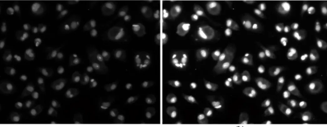
Figure 3.2: In this image are illustrated the implementation of global and local contrast stretching in Leishmania infected

images: a) Original grayscale image; b) Implementation of local limit contrast stretching. ... 10

Figure 3.3: Illustration of mathematical morphology operations in Leishmania infected images: a) original image; b)

dilation; c) erosion; d) opening; e) closing. The structuring element for all examples is a 5x5 square. The opening operation fails to eliminate the dot, because isn’t wide enough. ... 10

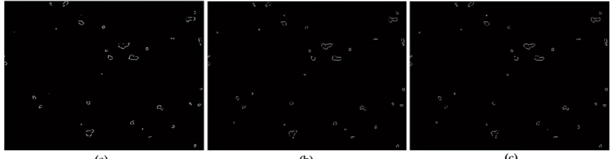
Figure 3.4: Illustrations of the some of the edge detectors in Leishmania infected images: a) Roberts Operator; b) Canny

Operator; c) LoG Operator. ... 12

Figure 3.5: Hough Transform detecting circles in a Leishmania infected image. ... 13 Figure 3.6: A bimodal histogram. The shaded areas show the effect of threshold variation on the area of the object [9]. 14 Figure 3.7: Illustration of the different thresholding implementation in Leishmania Infected images: a) Original Image; b)

Global thresholding implementation; c) Local Thresholding implementation d) Variance-based thresholding. ... 15

Figure 3.8: Illustration of the watershed segmentation in Leishmania Infected images: a) Watershed ridge lines; b) Markers

and object superimposed on original image; c) Color watershed label matrix. ... 16

Figure 3.9: Illustration of the K-Means segmentation in Leishmania Infected images: a) Cluster of parasites channel; b)

Cluster of nucleus channel; c) Label image of cluster index. ... 17

Figure 3.10: Illustration of the Mean-Shift segmentation in Leishmania Infected images: a) Original Image; b) Mean-Shift

implementation. ... 17

Figure 3.11: Segmentation output of a cluttered image. a) Original image; b) Adaptive multi-threshold output; c) Visual

representation of the cellular region vector obtained from the connected component analysis (randomly color-coded) [3]. ... 18

are depicted with different colors. ... 18

Figure 3.13: Results obtained from different phases of Neves et al. method: (a) Blob detection results; (b) K-means output;

(c) Binary Mask (adapted from [4]). ... 19

Figure 4.1: Study Design phases of this study. ... 23 Figure 4.2: Illustration of the image splitting result: a) Contrast stretched image; b) Macrophage nuclei channel (blue,

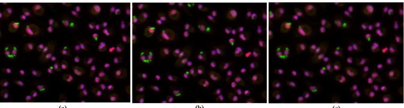
DAPI); c) Parasitic channel (green, Alexa 488); d) macrophage nuclei and cytoplasmic channel (red, Alexa568). Note that in b) and c) cytoplasmic regions are present, along with macrophage and parasite nuclei, respectively. This is due to the DNA to which each fluorophores binds itself... 24

Figure 4.3: Illustrations of Canny Operator edge detector and a closing operation in Leishmania infected images: a) Canny

Operator; b) Closing Operation. ... 25

Figure 4.4: Illustration of the normalization process: a) threshold image and b) opening operation result. ... 25 Figure 4.5: Schematic illustration of the four case studies performed in this study. ... 26 Figure 4.5: In this illustration it can be observed that two factors intervene in the image grouping, noise and clustering. So

the first subset refers to high noise and low clustering, the second one to high noise and high clustering, the third one to low noise and low clustering and the last one to low noise and high clustering. ... 26

Figure 5.1: Graph with global error ratio averages between case studies of all segmentation method implementation. .... 29 Figure 5.2: Graph with global error ratio averages between case studies of all segmentation implementations. ... 33 Figure 6.1: Images with some of the highest error ratio of segmentation in the used dataset due to image anomalies: a)

Photo-Bleaching phenomenon; b) Photon shot noise present in the right side of the image; c) Sample tampering anomaly; d) Auto-fluorescence phenomenon in the lower right corner of the image. ... 36

List of tables

Table 3.1: Summary results obtained from both Neves et al and Leal et al. methods. ... 19 Table 3.2::Summary of the related work in the literature [89]–[117]. ... 20 Table 4.1: The algorithms chosen for this study segregated by type. ... 24 Table 5.1: Global error ratio averages and standard deviation of structures segmentation in the nucleus channel for all case

studies in low noise images. ... 28

Table 5.2: Global error ratio averages and standard deviation of structures segmentation in the nucleus channel for all case

studies in high noise images. ... 29

Table 5.3: Global error ratio averages and standard deviation of structures under segmentation in the nucleus channel for

all case studies in low noise images... 30

Table 5.4: Error ratio averages and standard deviation of structures under segmentation in the nucleus channel for all case

studies in high noise images. ... 30

Table 5.5: Global error ratio averages and standard deviation of structures over segmentation in the nucleus channel for

all case studies in low noise images... 31

Table 5.6: Error ratio averages and standard deviation of structures over segmentation in the nucleus channel for all case

studies in high noise images. ... 31

Table 5.7: Global error ratio averages and standard deviation of structures segmentation in the parasites channel for all

case studies in low noise images. ... 32

Table 5.8: Global error ratio averages and standard deviation of structures segmentation in the parasites channel for all

case studies in high noise images. ... 32

Table 5.9: Global error ratio averages and standard deviation of structures under segmentation in the parasites channel for

all case studies in low noise images... 33

Table 5.10: Global error ratio averages and standard deviation of structures under segmentation in the parasites channel

for all case studies in high noise images. ... 34

Table 5.11: Global error ratio averages and standard deviation of structures over segmentation in the parasites channel for

all case studies in low noise images... 34

Table 5.12: Global error ratio averages and standard deviation of structures under segmentation in the parasites channel

for all case studies in high noise images. ... 35

Table 5.13: Time execution averages and standard deviations of all segmentation methods implementation in the different

1 Introduction

Leishmaniasis is a vector-borne disease caused by single-celled protozoans, usually transmitted by sand-fields.

It's characterized by their complexity and diversity [1]. Currently affects 12 million people in 88 countries, being

more prevalent in tropical and Mediterranean countries, including Portugal. The usual treatment for this

pathology is the administration of chemotherapeutics which are undesirable given their high degree of toxicity.

Although Leishmaniasis isn't life threatening in itself, it may seriously compromise the immune system, allowing

exposure too many other potentially fatal diseases [1]–[3].

Owing to these inadequate therapeutics, researchers have been addressing this problem with an attempt to

find a less aggressive and effective treatment [3]. Researchers are interested in determining the effect of drugs in

these infections [4].

Currently any biomedical research generates a large amount of microscope images. In most cases the analysis

is done manually and image by image [5]. As an example, one laboratory can produce thousands of images in one

day only by running 12 experiments [2].

The process in the analysis of images containing Leishmaniasis involves the recording of cells and parasites

in each image. Since each image contains hundreds of cells and parasites, the manual annotation takes a long

time, and is subjective and tiring [2]- [5]. Hence the motivation for automating the process of annotation.

Currently there are some solutions used in international laboratories. Some are commercial (Acapella [6]) and

others of free use (CellProfiler [7] and ImageJ [8]). While contemplating interesting computer vision algorithms

and a good performance, neither has a simple use. Researchers without programming knowledge have great

difficulty in handling it [5].

The aim of this study is to perform a comparative study between state of the art algorithms on segmenting

structures in fluorescence microscopic images infected with Leishmania.

Nine segmentation and two pre-processing algorithms were compared using four case studies. This case

studies are characterized by the lack or different pre-processing interventions. In order to evaluate this results an

error ratio metric was implemented.

The results of this research will enable a more precise and knowledgeable decision on setting up a

segmentation algorithm not only for Leishmania infected images but for all microscopic cellular images.

1.1 Thesis Outline

This document is organized in eight sections. The first introduces the issue, its characterization and its

context. The following two chapters describes additional information found in the literature, which is relevant

for the present work. The fourth section, outline the methodology and study design used during this research.

The fifth section presents the results for each implementation. In the sixth section, the results were discussed

with reference of the obtained results significance. Finally, the conclusion addresses the final considerations and

main achievements, study limitations as well as the proposed future work.

2 Cellular Biology Research

Why is cell biology one of the most crucial areas in clinical research? All living beings are constituted by cells.

So it becomes important to understand certain aspects of their physiology and metabolism, as well as of their

structure, origin, death and interaction with the surrounding environment.

This chapter addresses one of the most used tools in cell research, Fluorescence Imaging, applied to the field

of Leishmania research.

2.1 Fluorescence Imaging

Fluorescence microscopy is one of the most widely use tools in biological research. It enables the visualization

of cells and tissues, both in vivo and in vitro. Fluorescence imaging provides high selectivity and specificity of the

visualized structures due to fluorescent probes.

Due to the advancement of technologies, information systems and imaging techniques, fluorescence

microscopy has gained importance in the past years. From digital images it is possible to detect and analyze

microscopic structures in an automatic and precise way. This translates into a paradigm shift, from a qualitative

to quantitative analysis with precision. This is because previously digital images researchers conducted

quantitative analysis using only the naked eye in the microscope, which was proven not accurate and a biased

process.

Image processing provides numerical data enabling the massive and accurate quantification of microscopic

events that previously could only be qualitatively observed [9].

2.1.1 The Physical Principals of Fluorescence

One molecule can exist in a variety of states, which are determined by the configuration of its electrons and

vibration of its atomic nucleus [10]. Fluorescence occurs when certain molecules (called fluorophores,

fluorochromes or fluorescent dyes) absorb photons, reaching an unstable excited state, the singlet state (S1).

Under normal conditions, a molecule resides in stable ground state (S0), in its lowest vibrational and rotational

energy.

Whenever a molecule is excited, and the rotation of the electron is changed, the excited state is called a triplet

state. If the rotation stays unchanged the state is referred as a singlet state. The decay to the ground state of the

singlet results in fluorescence emission. Molecules in the S1 state can also undergo a spin conversion to the first

triplet state T1. Emission from T1 is designated as phosphorescence, and results in lower energy emission (see

Figure 2..1) [9], [11].

Fluorescence occurs when the excited molecule returns to its ground state by releasing energy (photon

emission). After absorbing photons, some of the energy is converted into heat, thus explaining the difference in

wavelength observed in Figure 2.2 [9], [10]. This phenomenon is called the Stokes shift. The fluorophores that

exhibit a spectrum with a higher Stokes shift are ideal, because the light that they emit is easily separated from

the excitation light via optical filters [10]. The energy of the emitted photon equals the difference between the

energy levels of the states of excitation and emission, and determines the wavelength of the light emitted, 𝜆

,

as follows:

𝜆𝐸𝑀=

ℎ𝑐 𝐸𝐸𝑀

(2.1)

where E

is the difference between the levels of energy states during light output, h is Planck's constant and

c is the speed.

Emitted fluorescence can be expressed as:

𝐼𝐸𝑀= 𝐼𝐸𝑋∙ 𝜀 ∙ 𝑐 ∙ 𝑥 ∙ 𝜙

(2.2)

where 𝐼

is the light intensity, 𝜀 is the coefficient of the fluorophore excitation, c is the concentration of the

fluorophore, x is the optical path length and φ is the quantum efficiency. This reflects the ability of fluorophores

to convert the absorbed light into emitted fluorescence [9].

Figure 2.1:Jablonski diagram representative of transmission between levels of electrons energy. After the absorption of a photon

with a specific wavelength, the molecule changes from its ground state to an excited state. Then the vibrational energy is converted into heat, which is called the vibration relax process or internal conversion. When the molecule returns to its ground state the reminiscent energy is released by the emission of a new photon with a longer wavelength, resulting in fluorescence emission (adapted from [11]).

2.1.2 Instrumentation of fluorescence imaging

Fluorescence microscopy can be performed on various types of microscopes, namely wide field, confocal and

two-photon. To do so, these must be properly equipped. The illumination source must be able to excite the

fluorophores. In other words, be capable of emitting light with specific wavelengths. Normally white light is

used, because it contains all the wavelengths of visible light at approximately equal intensities. The selection of

these specific wavelengths is accomplished by using an excitation filter in the path of excitation light and an

emission filter on the path of fluorescence emitted. It is also necessary that the excitation and emission lights are

properly separated and subsequently detected. The separation of the reflection light excited and emitted is

possible by using a dichroic mirror, as seen in Figure 2.2. and 2.3.

Figure 2.2:Representation of the profile of the absorption and emission spectrum of the fluorophore with the relative intensities

and corresponding wavelengths [2].

2.1.3 Image Formation

Fluorescence microscopy features an incoherent imaging process due to random re-emission of photons.

This is so because each sample point has an independent contribution in the distribution of light intensity within

Each fluorophore in the sample acts as a light source thus allowing the principle of superposition. So image

acquisition occurs by integrating all of these secondary light sources [9], [10]. The resulting images by fluorescence

microscopy can be modeled as a linear and invariant system in space [10], [12], [13].

Figure 2.3: Schematic illustration of the necessary components in fluorescence microscopic [3].

2.1.4 Fluorophores

Fluorophores are chemical fluorescent compounds that are able to emit light after being excited with light of

specific wavelength. Fluorophores can be divided into two major classes, intrinsic and extrinsic. Intrinsics

correspond to those that occur naturally, while extrinsics are added to the samples, in order to add fluorescence

properties in the sample spectrum [11]. It is possible to specifically bind different fluorophores to distinct

macromolecules. Depending on the excitation and emission characteristics of the fluorophores, these will be

detected in different light channels. In other words, the use of different fluorophores in the same biological

sample may allow the simultaneous visualization of different microscopic structures with different colors.

2.1.5 Limitations of Fluorescence imaging

The equipment used nowadays in microscopy is built to minimize optical aberrations and phase distortion.

Yet no system is free from optical distortions and defects. The sources thereof can be divided into two categories:

instrumentation-based and sample-based.

2.1.5.1 Instrumentation-based Anomalies

The selection of the system configuration in fluorescence microscopy greatly contributes to the quality of the

acquired images. This includes the light source, lenses, excitation and emission filters, as well as the photosensitive

detectors.

Light sources should be stable and generate a uniform and reproducible field. The quality and performance

of the objective lens is directly associated with the system resolution. So it is necessary to choose the best for

each individual case. Likewise, detectors must be chosen to ensure that the Nyquist limit is satisfied [14]–[16].

Despite how often the best instruments are chosen to have optimal results, there is always inherent noise in the

images.

One major limitation that arises in fluorescence imaging is the photon shot noise. This artifact results of the

natural and random emission of photons. The absorption of photons by photo-detectors creates photoelectrons

and instead of cashing them out of the photo-detector counts them. Although there are means to circumvent

this, as the integration time and the quantum efficiency of photo-detectors, the nature of random photons is

impossible to avoid. The noise is independent of the electronic equipment and can be reduced by increasing the

exposure time of the sample and the light intensity.

Photo-detectors also originate another type of noise, known as dark current. This matches the number of

electrons induced by pixel, which results from thermal agitation. The thermal energy is the main reason for the

appearance of this noise. The higher the temperature, the greater will be the kinetic energy of the electrons and

subsequent induction of these per pixel. For the photo-detectors this noise occurs when the integration time or

temperature values are too high. [14]–[16].

Other devices associated with the photo-detectors cameras can generate noise during the readout of the

values. When the reading frequency is high this sort of noise becomes additive that might become problematic.

All digital detectors produce quantization noise. This noise is inherent to the amplitude of the quantization

process. This takes place in analog to digital signal conversion. It is signal independent and can be modeled as an

additive noise, when the dynamic range of intensity is equal or less than 2

_.

2.1.5.2 Sample-based Anomalies

Sample characteristics will determine not only the image formation but also the introduction of anomalies.

The most frequent anomalies are photo-bleaching, auto-fluorescence, absorption and scattering

Photo-bleaching causes an effective reduction and often a complete elimination of fluorescence emission. On

a molecular level, photo-bleaching occurs when an electron reaches the triple excited state that has longer

duration, thus allowing a chemical reaction between the labelled molecule and the fluorophore to occur. This

process results in permanent changes in the fluorophore which affect the ability to emit fluorescence or absorb

the excitation light with the same wavelength (See Figure 2.4).

Figure 2.4: Example of photo-bleaching phenomenon in a fibroblast cell. Over time the green fluorescence has faded and the red

fluorescence is virtually unchanged. [17].

Auto-fluorescence occurs when some organic or inorganic molecules are naturally fluorescent. This

phenomenon is a significant source of background noise in fluorescence images. In quantitative research it is

problematic because it creates anomalies in the images due to the overlap of the fluorescence concerning the

fluorophore and auto-fluorescence molecule.

Absorption and scattering of light are common causes of optical anomalies observed in fluorescence imaging.

Light at wavelengths of emission and also excitation can be scattered due to particles present in the sample, or

refracted due to interfaces and even absorbed by the sample material [9], [10].

2.2 Leishmania

Leishmaniasis is a spectrum of diseases that affects dogs and humans and that are caused by the protozoan

parasite Leishmania. Leishmaniasis is transmitted by the bite of phlebotomine sandflies. The life cycle of this

parasite is divided between the insect vector and the mammalian hosts. Inside mammals, Leishmania resides in

macrophages (cells of the immune system). After their invasion the parasite begins to reproduce until the

macrophage ruptures. Subsequently they will invade other cells of the mammal contributing to the disease

progression [1].

Leishmaniasis can have a wide range of clinical symptoms, which may be cutaneous, mucocutaneous or

visceral (See Figure 2.5). Cutaneous leishmaniasis is the most common form. Visceral leishmaniasis is the most

severe form, in which vital organs of the body are affected [18].

These maladies currently affect 12 million people in 88 countries, being prevalent in tropical and subtropical

areas of the globe, as well as in Mediterranean countries, including Portugal [18], [19]. The usual treatment for

this pathology is the administration of chemotherapeutics which are far from being ideal.

Among the reasons that justify this we have a high degree of toxicity of this treatment, and the fact that the

incidence of this pathology affects countries with minimal access to primary care which hampers their

administration.

Figure 2.5: Illustration of the different clinical symptoms of leishmaniasis: mucocutaneous, cutaneous, and visceral, respectively

(adapted from [7]).

Certain forms of Leishmaniasis are life threatening and those who are not, may seriously compromises the

immune system, allowing exposure too many other potentially fatal diseases [2], [3], [19].

Research on Leishmania can cover different topics, including, among others, the study of unique aspects of

parasite biology and/or mechanisms of parasite interaction with its mammalian host, and the testing of new

anti-parasitic compounds with potential therapeutic applications [3] [2].

2.2.1 Leishmania Research

Fluorescence microscopy of Leishmania-infected macrophages is widely used in Leishmania research. In order

to distinguish Leishmania from its host cells, specific fluorophores are used. For marking parasites, researchers

combine a Leishmania-specific antibody and the Alexa Fluor 488 dye. This fluorophore, characterized by an

excitation maximum of 493nm and an emission maximum 517nm, translates into an emission of a green color.

To identify macrophages, researchers use Propidium Iodide (PI), a dye with an excitation maximum of 305nm

and an emission maximum of 617nm [20], that confers red color to the molecules it binds to. Propidium iodide

binds to DNA and RNA, thereby labeling the macrophages and the parasites nuclei, as well as the Leishmania

mitochondrial DNA (the kinetoplast). The macrophage nucleus can be easily distinguished from that of the

parasite, because the latter is much smaller. Since PI also marks RNA, it is possible to observe shades of red in

the macrophage cytoplasm, the cell compartment that accommodates this type of molecules. As an alternative

to PI, researchers can use DAPI to label DNA. Contrary to PI, this dye does not bind RNA. It is characterized

by an excitation maximum of 359nm and an emission maximum of 457nm, and emits in blue.

Fluorescence micrographs of Leishmania-infected macrophages can be used for various purposes, among

which the estimation of infection parameters. These include the percentage of infection (PI), the number of

parasites present in each infected cell (NPI) and infection index in cells (IX). These measurements are determined

by counting the macrophage and parasites present in the images. Traditionally this was manual counting,

performed by researchers. Today some software assists in this work.

2.2.2 Software Tools

Currently there are some solutions used in international laboratories that assist in this work. Some are

commercial (Acapella[6]) and others of free use (CellProfiler [7] and ImageJ [8]). Even though they contemplate

interesting computer vision algorithms and a good performance, they are not simple to use. Researchers without

programming knowledge have great difficulty in handling it [5] .

In 2008 the Faculty of Sciences of the University of Porto along with the Institute for Molecular and Cell

Biology started to develop the CellNote software. Today CellNote is capable of automatic annotation and analysis

of microscopic images in desktop computers. The projects leaders are Miguel Coimbra in Computer Vision

Group and Helena Castro in Molecular Parasitology Group [21].

João Faustino Ribeiro

Medical Informatics Dissertation 8

3 Cellular Microscopic Image Processing

Over the last years microscopy imaging and image processing have been subject of interest of scientific and

engineering communities. Recent developments in cellular, molecular technologies on a nanometric level led to

fast breakthroughs and push the boundaries of human knowledge in biology, medicine, chemistry, pharmacology,

and many related areas. Microscopes have long been used to capture, observe, measure and analyze images of

various living microorganisms or structures in scales far below of human visual perception. With the advent of

affordable technologies, high computing performance and image sensors, digital imaging came into prominence.

Digital image processing is a natural extension, because it’s proving to be essential to the success of subsequent

data analysis and interpretation of microscopic images. The digital image processing and computer vision

processes opened new fields of medical research and brought the possibility of advanced diagnostic clinical

procedures [9].

This chapter describes the methods most commonly used in the cellular image processing as well as methods

that in last years have showed great results in similar applications. They will be addressed in sections,

pre-processing and segmentation respectively.

3.1 Pre-processing

Preprocessing can be defined as any data transformation prior to the construction of a model that relates all

data with the world. These transformations are often heuristics. The parameters are sometimes chosen for

convenience or experience and not by training data. The image data can depend on many aspects of the real

world, but these are not mandatory to the task at hand. The major goal of preprocessing is to remove the

maximum of unwanted variations as possible while maintaining the integrity of all important aspects to the task.

Preprocessing is one of the most important task in a computer vision system, so it is very important to analyze

the most prominent techniques in this field in order to choose the most adequate [22].

3.1.1. Noise Smoothing Filters

Image filtering’s main objective is to remove/conceal noise of the image in order to improve its quality or

highlight some desirable features [23].

Low pass filtering is often regarded as the elimination of high frequencies in the signal. Therefore it is natural

to perform it in the frequency domain. However, you can apply it directly in the spatial domain. This is possible

because a signal multiplied by a function in the frequency domain is equivalent to the convoling their inverse

Fourier transformed versions in the spatial domain. [24]. If the final convolution function in the spatial domain

is sufficiently narrow, the amount of computation involved is not excessive. Marr and Hildreth suggested that

the appropriate type of filter to use are those that are well-behaved (nonoscillatory), both in frequency and space

domains. [25]. Gaussian filters meet ideally this criterion because they have identical shapes in spatial and

frequency domains, and it can be defined mathematically in 2D as:

𝐺(𝑥, 𝑦) = 𝑒 −𝑥 2_+𝑦2 2𝜎2 2𝜋𝜎2 (3.1)

σ corresponds as the standard deviation of the Gaussian (or its “sigma”), the units are inter-pixel spaces,

usually referred to as pixels [26].

Sometimes an interference occurs during the process of image acquisition and this can lead to an impulse or

"peak" of noise. That peak corresponds to intensities completely wrong of an individual group of pixels. Since

the Gaussian filter is a sliding average, its application may result in a distortion of all the intensities values.

To solve this problem, one option would be exploring and locating the image pixels that have extreme and

unlikely intensities. These would be ignored and replaced with more appropriate values. The most obvious option

to achieve this is to apply a threshold filter that prevents any pixel having a very disparate intensity of its

neighbors. Then it would be necessary to analyze the local intensities distribution of a given neighborhood. If

they are in areas with peak intensities, they will be removed and the search and removal of identical areas was

made. Thus we arrive to the median filter, which analyzes the entire intensities distribution of local pixel and

subsequently generates an image corresponding to the set of its median value [23] [27]. The literature highlights

this filter’s advantages towards the Gaussian filter due to computation spending and the previously mentioned

problem [28]–[30].

Since the Gaussian and median filters were referred it would be normal to analyze and describe the mode

filter. The only problem is that almost all images under consideration follow a multimodal distribution, which

prevents its use [23].

Figure 3.1: Illustration of a Gaussian and median filters implementation in Leishmania infected images: (a) Original Image; (b)

Gaussian filter implementation; (c) Median filter implementation.

3.1.2. Contrast Stretching

Display devices usually have a limited number of gray levels that often comprise the image features, hindering

many post processing tasks. So global adjustment methods are required to ensure that the interest characteristics

are in the visible range. This technique is designated as contrast stretching. If the intensity variation of interest is

between 𝐼

and 𝐼

, a scaling transformation can be performed to map the intensity of the original image, I, for

the image g, with a range of 𝐼

to 𝐼

:

𝑔 = 𝐼 − 𝐼1 𝐼2− 𝐼1

(𝐼𝑚𝑎𝑥− 𝐼𝑚𝑖𝑛) + 𝐼𝑚𝑖𝑛 (3.2)

This mapping is a linear stretching transformation. A series of nonlinear monotonic pixel operations can also

be performed. For example, the following transformation maps the gray level of the image according to a

nonlinear curve:

𝑔 = (

𝐼 − 𝐼

𝐼

− 𝐼

)

(𝐼

− 𝐼

) + 𝐼

0 < 𝛼 < ∞

where 𝛼 is an adjustable parameter. This image intensity scaling is usually used for contrast stretching,

clipping, display calibration, etc [9], [31].

(a) ) (b) ) (c) a))

Figure 3.2: In this image are illustrated the implementation of global and local contrast stretching in Leishmania infected images: a) Original grayscale image; b) Implementation of local limit contrast stretching.

3.1.1 Mathematical Morphology

Morphological processing has applications in many areas of image processing such as filtering, segmentation

and even post-processing in binary and grayscale images. One of the biggest advantages of morphological

processing is the inherent structure blocks, where complex operators can be created by composing some

primitive operators. Moreover, each of these primitive operators have an intuitive physics that helps a lot to

understand the effects that can be produced in an image.

Morphological image processing is based on the survey of an image with a structuring element that can filter

or quantify the image according if the same could fit or not into the image.

The operations of image processing used in most binary images are collectively referred to as morphological

procedures. These include erosion, dilation, and modifications and combinations of these two techniques [32]–

[36]. Such operations can be easily described with the addition and removal of pixels in a binary image according

to certain rules.

Figure 3.3: Illustration of mathematical morphology operations in Leishmania infected images: a) original image; b) dilation; c)

erosion; d) opening; e) closing. The structuring element for all examples is a 5x5 square. The opening operation fails to eliminate the dot, because isn’t wide enough.

The basic operation of mathematical morphology is the erosion of an image by a structuring element. The

result of erosion is the removal of all the “sections” where the structuring element “does not fit” within the

(a) ) (b) ) (e) ) (c) ) (d) ) (a) ) (b) )

controlled by the size and shape of the structuring element. The erosion of the set A by set B is defined as:

𝐴 ⊖ 𝐵 = {𝑥: 𝐵𝑥⊂ 𝐴} (3.4)

where ⊂ denotes the relationship of the subset A and 𝐵

= {𝑏 + 𝑥: 𝑏 ∈ 𝐵} and translating the set B for a

point 𝑥.

Contrary to erosion, dilation adds pixels to a binary image. The dilation of the set A by set B is defined as:

𝐴 ⊕ 𝐵 = {𝐴𝑐_{⊖ 𝐵̆}}𝑐 _(3.5)

where 𝐴

_{denotes the complement of 𝐴 and 𝐵̆ = {−𝑏: 𝑏 ∈ 𝐵} is the reflection of 𝐵, that is, a rotation of}

180º of original 𝐵.

The combination of these two operations is very common in practice. The combination of an erosion

followed by a dilation is designated an opening because it is used for the removal of fine and isolated lines. If

conversely to execute this operation is referred to a closure for closing breaks in features. [22], [37].

3.2 Segmentation

One of the first tasks to be undertaken in any computer vision system after preprocessing is segmentation,

which divides the image into a number of uniform regions (texture, brightness and color), and thus enhances the

region of interest. The construction of a segmentation algorithm always takes into account that each object is

subject to a level of uniformity (whether on its intensity, texture, or other aspects), although this decision is

actually semantic (e.g. Is this pixel part of that cell nucleus?). Although the human eye distinguishes objects within

an image just by one glance, a number of different processes are carried out by our cognitive system that allow

us to do so. Thence the segmentation process is one of the central problems of any computer vision system. In

this subsection, we analyze the segmentation techniques with interest for cellular images with some illustrative

demonstrations.

3.2.1 Edge Detection

The first step of image interpretation in many strategies is detecting edges. Generically an edge consists in a

group of pixels interconnected separating two homogeneous regions. So, these can be defined as sudden changes

in pixel intensities and thus reflecting on the gradient [23], [26], [37], [38].

3.2.1.1 Edge Detection Operators

The ultimate goal of edge detection is to highlight the pixels that have abrupt changes of gray levels. For this

it is necessary to analyze the direction and inclination responsible for this change. An operation of convolution

of each image pixel, I(x, y), by a mask/kernel (differentiation of first order) is used. With these operators it is

possible to quantify the inclination (often also its direction) of the gray level transitions. The majority of these

operators performs a measurement of the spatial gradient in 2D through the convolution of two kernels, 𝐺

and

𝐺

. Each pixel suffers a convolution with each of the two kernels, where one estimates the x gradient direction

and the other the y gradient direction [9].

The result of these operations can be combined in order to estimate the maximum gradient magnitude, |𝐺|,

and its orientation, 𝜃, at each pixel.

|𝐺| = √𝐺𝑥2+ 𝐺𝑦2 (3.6)

where 𝐺

and 𝐺

are the result of the derivation function of the x and y directions:

𝐺𝑥= 𝐼(𝑥, 𝑦) × 𝑔𝑥 and 𝐺𝑦= 𝐼(𝑥, 𝑦) × 𝑔𝑦

𝜃 = 𝑎𝑟𝑐𝑡𝑎𝑛 (𝐺𝑦 𝐺𝑥

) (3.7)

Over the years, a number of operators that are able to find edges have been proposed. Under the most

popular, there are: Roberts, Prewitt, Sobel, Kirch and Canny [39]–[43].

The major problem with the use of kernels based on the first derivative to find edges is to determine with

certainty the best threshold value to classify a pixel as edge or not. With the application of second derivative this

is easier since edges are reflected as signal changes. TheLaplacian operator is based on second derivative and can

be defined mathematically as:

∇2_{𝐼 =}𝜕2𝐼

𝜕𝑥2+

𝜕2_𝐼

𝜕𝑦2 (3.8)

The Laplacian has the advantage of being an isotropic measure of the second derivative. The magnitude of

the edge is independent of the direction and can be obtained by the convolution of the image with the following

kernel:

The major disadvantage of this operator is the high noise sensitivity. Due to this it is necessary to apply

smoothing operations along with this operator. A Gaussian filter is usually used. Because the convolution process

is associative it’s possible to combine these two operations, being designated as Laplacian of Gaussian (LoG)

and mathematically described:

𝐿𝑜𝐺(𝑥, 𝑦) = −∇2_{𝐺(𝑥, 𝑦)} = −∇2 1 2𝜋𝜎2𝑒 −𝑥 2_+𝑦2 2𝜎2 = 1 𝜋𝜎4[1 − 𝑥2_{+ 𝑦}2 2𝜎2 ] 𝑒 −𝑥 2_+𝑦2 2𝜎2 (3.10)

This combination was proposed by Marr and Hildreth in 1980, being known also by their names [25].

Figure 3.4: Illustrations of the some of the edge detectors in Leishmania infected images: a) Roberts Operator; b) Canny Operator; c) LoG Operator.

3.2.1.2 Hough Transform

The shape of the desirable detecting structure is known a priori on several occasions. In 1959, Hough proposed

a method to detect lines in an image. He published his work as a patent for an electronic device for detecting

particles of high energy tracks [44].

The Hough transform basic concept in line detecting is the duality between points and lines. A point, P, can

be defined in space by a certain coordinate, (x, y), or by a set of lines that pass through him. If we analyze a set

of collinear points, 𝑃𝑐, of the point 𝑃 and at the same time list of sets of lines passing through these points

individually, we note that there is a common line to all these points. Therefore it is possible to find the line that

contains all the points 𝑃𝑐 and discard the rest. Such forwent is easily observed because if we mix a set of noise

points, 𝑃𝑛, this method is able to discriminate them from the collinear points.

Originally, in order to parameterize lines from points, this method used the slope-intercept equation:

y = 𝑚𝑥 + 𝑏 (3.11)

Each point on a straight line is then drawn as a line in

space corresponding to all

values. The

embarrassment of unlimited values ranges (nearly vertical lines that require almost infinite values of

parameters) is surpassed by using two set of graphics, the first corresponds to slopes less than 1.0 and the second

one to slopes up to 1.0 or more [23]. Due to this need Duda and Hart in 1972 proposed a change in the

parameterization forms of Hough transform using polar coordinates:

ρ = 𝑥 cos 𝜃 + 𝑦 sin 𝜃 (3.12)

where ρ is the length of the line and 𝜃 is the angle to which x and y are subject [45].

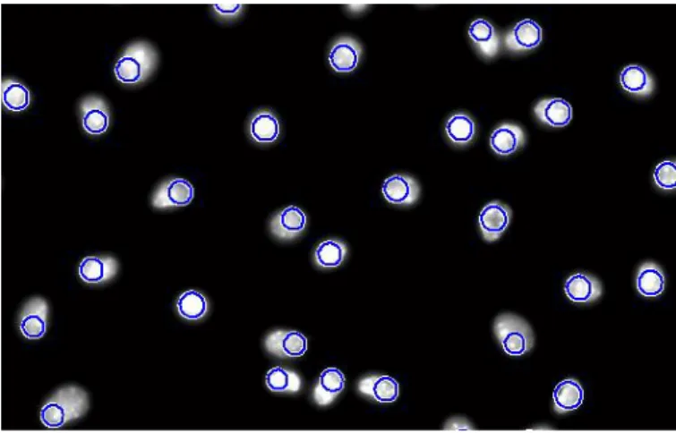
Figure 3.5: Hough Transform detecting circles in a Leishmania infected image.

Over the years, upgrades and derivations of the original transform have been proposed. in 1986, Davies

proposed the adjustment to circles and in 1989 Yuen to ellipses [46], [47]. As the Hough transform is an extremely

general procedure, a generalization of the same has been proposed in order to detect a large number of image

features and this work was mainly due to Farber in 1975 and Barllard in 1987 [48], [49].

In theory, the method works, but in practice it’s very difficult to use, even for line detection, because of the

long processing time, the quantization errors and noise related problems [26].

3.2.2 Thresholding

The most traditional segmentation technique is thresholding, because of its intuitive properties and its

implementation simplicity. In this technique we choose a threshold value and check each pixel whether the

intensity values are above or below, thus dividing the image into two distinct regions.

The threshold selection is crucial to this technique’s success. Unless the object in the image has edges with

high contrast, any variation of the threshold value can significantly affect the object edge position and therefore

the object total size.

An image that contains an object typically has a bimodal histogram of gray levels (see figure 3.1). The peaks

correspond to the object and background, and the dip between them corresponds to a group of pixels near the

object edge. When a threshold value, 𝑇, is selected, the area of the object is given by:

𝑎𝑟𝑒𝑎 = ∫ 𝐻(𝐼) 𝑑𝐼

𝑇 0

(3.13)

where 𝐻(𝐼) is the image histogram.

Figure 3.6: A bimodal histogram. The shaded areas show the effect of threshold variation on the area of the object [9].

Although there isn’t an universal method for threshold selection, a variety of techniques have been developed

for different circumstances [50], [51]. Among others, we have histogram smoothing, the isodata algorithm,

background symmetry, triangle algorithm and gradient-based algorithms.

The most intuitive approach of thresholding is the global thresholding, because it’s the simplest and quickest.

This has a relatively good performance in images with objects of similar intensities, or when the contrast between

the object and the background is high. However, this process cannot be considered automatic and accurate,

because in the same image it can be found different tissues with similar intensities and this process doesn’t

distinguish them, it only divides the image only into two regions. The accuracy of the object edges is also

questionable, because the threshold value can be subject to large statistical fluctuations (image artifacts). With

the increase of noise or low contrast, the threshold selection becomes more and more difficult. Mathematically

we can describe the thresholding operation as:

𝐺(𝑥, 𝑦) = {𝐹 𝑖𝑓 𝐼(𝑥, 𝑦) ≥ 𝑇

𝐵 𝑖𝑓 𝐼(𝑥, 𝑦) < 𝑇 (3.14)

where 𝐼(𝑥, 𝑦) corresponds to the original image, 𝑇 is the threshold value, 𝐹 the foreground and 𝐵 the

background [9].

Besides the global thresholding, there are other thresholding methods such as local thresholding, adaptive

thresholding and Variance-Based Thresholding. These techniques are used when the threshold value cannot be

determined from the histogram analysis, or just a single threshold value cannot get a good image segmentation.

The local thresholding method uses a threshold value calculated for each pixel. This value can be determined

from the average value, the intensities distribution, or by statistics such as average, maximum and minimum

values, amongst others.

Due to uneven lighting and other factors, the contrast between the object and the background varies within

the image. In these cases, global thresholding is unlikely to obtain positive results, since the threshold value only

works well in a portion of image. To cope with this variation, we can used an adaptive or variable threshold value.

Over the years various methods have been proposed by Chow and Kaneko in 1972, and more recently by Liu et

al in 2002 [52], [53].

Previously it was mentioned that the success of any thresholding operation is dictated by the choice of the

threshold value. However, sometimes it becomes impractical when we analyze the histogram and the existing

peaks are tiny and impossible to distinguish from some noise peaks. In this situation it is impossible to extract

the threshold value by traditional algorithms. Over the years, this issue has been addressed by several researchers

[50], [54]–[56].

The variance-based thresholding is characterized by the histogram analysis and extraction of small sections

for further analysis, in order to optimize the threshold selection. The simplest and most robust approach was

proposed by Otsu in 1979, which corresponds to the calculation of the variation between classes [54].

First it is assumed that the image has a resolution of 𝐿 gray levels. The number of pixels with gray levels is

called 𝑛

, and the total number of pixels in the image corresponds to 𝑁 = 𝑛

+ 𝑛

+ ⋯ + 𝑛

.So, the probability

that a pixel having a gray level translates to:

𝑝𝑖=

𝑛𝑖

where

𝑖≥ 0 𝑒 ∑ 𝑝𝑖 𝐿 𝑖=1

= 1

For intervals greater or smaller than the threshold value,𝑘, the variance between classes, 𝜎

, and the total

variance, 𝜎

, can be calculated by the following equations:

𝜎𝐵2= 𝜋0(𝜇0+ 𝜇𝑇)2+ 𝜋1(𝜇1− 𝜇𝑇)2 (3.16) 𝜎𝑇2= ∑(𝑖 − 𝜇𝑇)2𝑝𝑖 𝐿 𝑖=1

Where,

Using equations previously mentioned, the variance between classes can be simplified:

𝜎𝐵2= 𝜋0𝜋1(𝜇1− 𝜇0)2 (3.17)

We can use this technique for two threshold analysis [23].

Figure 3.7: Illustration of the different thresholding implementation in Leishmania Infected images: a) Original Image; b) Global

thresholding implementation; c) Local Thresholding implementation d) Variance-based thresholding.

3.2.3 Clustering Techniques

Clustering is a process that agglomerates data according a feature and thus form one or various clusters. It’s

then natural to think about image segmentation as clustering, i.e., we can represent an image in terms of pixel

clusters. The specific criterion of similarity used depends on the application. It could be the color, texture,

neighborhood, among many others. Each image is characterized by a set of pixels and a feature vector can

represent each of them. This feature vector contains all measures that may be relevant to describe a pixel. Natural

(a) ) (b) ) (c) ) (d) )

feature vectors include: the intensity, localization and color of the pixel, and a vector of an output filter

representative of the local texture.

Each feature vector belongs to exactly one cluster and this is characterized as an image segment. We can

obtain the image segment represented by a cluster by replacing the number of the feature vector at each pixel

with the number of feature vector of the central cluster. This method is extremely general, a choice from the

different feature vectors will generate different types of image segments and consequently different clusters.

Clustering can be characterized by two natural algorithms, agglomerative and divisive. The agglomerative

takes a bottom-up approach, since each pixel is classified as a cluster, these will suffer agglomerations until the

stopping criterion is reached. The divisive has a top-down approach, i.e., the total number of image pixels is

classified as a cluster that suffers successive divisions until a stopping criterion it’s reached [26].

3.2.3.1 Watershed Segmentation

Watershed segmentation method has been greatly developed for a large number of situations in the real world,

and a number of algorithms have been implemented [57], [58]. Watershed algorithm was designed and proposed

by Beucher in 1979, which suffered some adjustments in 1990 [59], [60].

This algorithm calculates the gradient magnitude of the image map 𝐼, ‖𝛻𝐼‖. The zero’s of this map are

intensity values of local extremes that are seeds for each segment. Each seed will have a unique label. Next, each

pixel will be assigned to a seed using a procedure analogous to the filling height map with water (hence the name,

Watershed). That is, the pixel, (𝑖, 𝑗), will only match a single seed, if we backward travel down the gradient of

‖∇𝐼‖

. Hence this method is classified as agglomerative, because initially there are seed clusters and later a number

of pixels are agglomerated to them.

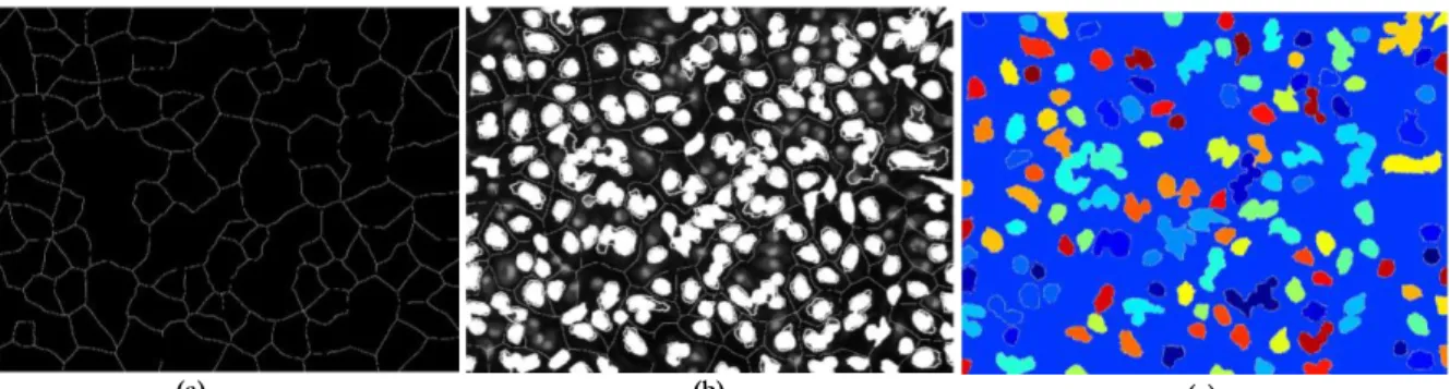
Figure 3.8: Illustration of the watershed segmentation in Leishmania Infected images: a) Watershed ridge lines; b) Markers and

object superimposed on original image; c) Color watershed label matrix.

3.2.3.2 K-means Segmentation

K-Means is an unsupervised clustering algorithm that assigns pixels into different classes based on their

inherent distance from each other. It was proposed by Stuart Lloyd in 1982 and later extended by Pelleg and

Moore in 2000 [61], [62]. This algorithm tries to find natural clustering. The pixels are clustered around centroids

𝜇

∀𝑖 = 1 … 𝑘 which are obtained by minimizing the objective:

∑ ∑ ‖𝑥𝑗− 𝜇𝑖‖ 2 𝑥𝑗∈𝑆𝑖 𝑘 𝑖=1 (3.18)

where there are 𝑘 clusters 𝑆

= 1, 2, … 𝑘 and 𝜇

is the centroid or mean point of all the points 𝑥

∈ 𝑆

[63].

For cluster formation/analysis it’s based in statistical methods. This produces good results of image

segmentation for some particular applications. The main drawback of this method is the fact that the user defines

the number of clusters, which could cause a bias result [26].

(a) ) (c) ) (b) )

Figure 3.9: Illustration of the K-Means segmentation in Leishmania Infected images: a) Cluster of parasites channel; b) Cluster of

nucleus channel; c) Label image of cluster index.

3.2.3.3 Mean Shift Segmentation

Mean shift is a non-parametric technique that was proposed by Hostetler and Fukunaga in 1975 [64]. Consists

in the analysis of a complex multimodal space features and estimate stationary points of the underlying density

function.

In 2002, Comaniciu and Meer proposed a segmentation method using the mean shift algorithm [65]. This

assumes that the clusters correspond to local maximum density (local modes). It’s used a smoothing kernel, in

order to obtain an approximate representation of the image density. Clustering with mean shift algorithm is

simple, in principle. This method will attribute a mode to each pixel. Being this a continuous variable it’s expected

that all modes are different but at the same time, clearly grouped. In order to cluster this pixels, it is applied a

simple agglomerative algorithm. The decisive parameter of clustering is the mode’s mean distance with a

threshold value (that acts like a stop criteria of the agglomerative algorithm) [26].

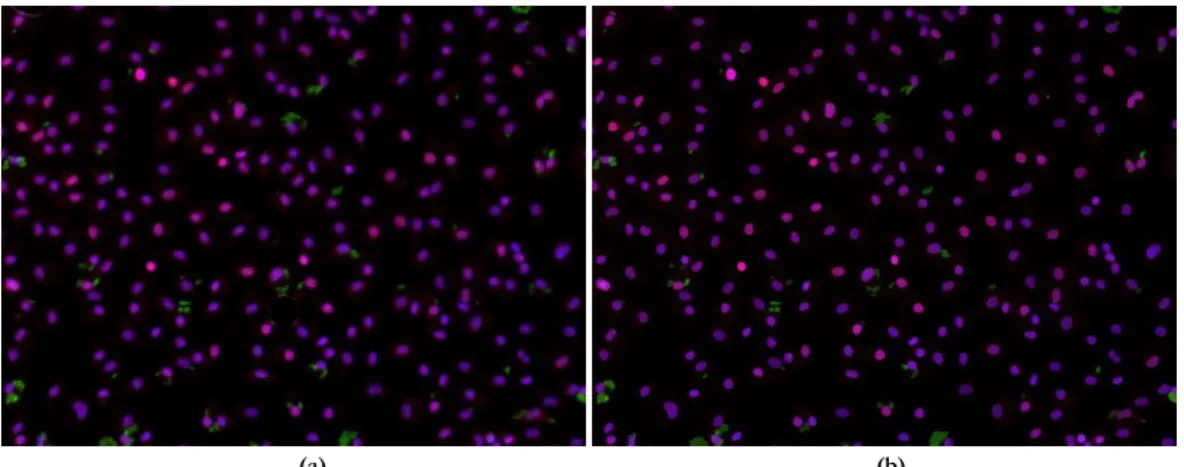
Figure 3.10: Illustration of the Mean-Shift segmentation in Leishmania Infected images: a) Original Image; b) Mean-Shift

implementation.

3.3 Related Work

During the last decade, many efforts have been made on automatic segmentation of cellular structures from

microscopic images, such as simple thresholding [66], [67], region-based segmentation highlighting the watershed

algorithm [65], [68]–[73], contour-based models segmentation [74]–[77] and unsupervised and supervised

machine learning techniques [78]–[86]. One area of particular interest is blood cells segmentation and

subsequently their counting for immunological purposes. In Table 3.2 are the most recent and relevant studies

present in the literature concerning segmentation and classification methods of cell structures in microscopy

images.

To the best of our knowledge, the automatic annotation of Leishmania infections in fluorescence microscopy

was only addressed in three different approaches: Leal et al., Nogueira et al. and Neves et al. [3], [4], [87].

(a) ) (c) ) (b) ) (a) ) (b) )

Figure 3.11: Segmentation output of a cluttered image. a) Original image; b) Adaptive multi-threshold output; c) Visual

representation of the cellular region vector obtained from the connected component analysis (randomly color-coded) [3].

Nogueira et al. in 2012, using computer vision and pattern recognition methodologies, proposed an algorithm

to determine automatically infection indexes of macrophages parasite by Leishmania in microscopy image [3]. This

begins by performing a contrast stretching operation for readjusting illumination conditions. In order to identify

the parasites and the macrophages nuclei, an adaptive multi-threshold (Otsu’s method) it’s applied parameterized

with a different constraints vectors. Regions with multiple nuclei or parasites are processed by a voting system

that employs both a Support Vector Machine and a set of region features for determining the number of objects

present in each region. The previous vote is then taken into account as the number of mixtures to be used in a

Gaussian. The correspondence between each parasite and one or more macrophages is performed using a

minimum Euclidean distance to a cell’s nucleus, quantifying Leishmania infection levels. Nogueira et al. method

was able to count macrophages and parasites with >90% accuracy and de-cluster regions with multiple nuclei

and parasites with a 75-85% accuracy [3].

Leal et al in 2012 used the Difference of Gaussians (DoG) filter to enhance the parasites and macrophages

at the desired scale. An iterative process combined with an adaptive threshold method was used in order to tune

the value of standard deviation of DoG to the scales of macrophages nuclei/parasites present in the image. Next,

the blue and green channel were filtered to obtain the locations of macrophages nuclei and parasites, respectively.

These locations were used not only as the result of automatic annotation but also as seeds to the watershed

algorithm. The watershed algorithm segments the cytoplasm of the macrophages, so that a more accurate

association between macrophages and parasites can be achieved. This approach was successful and has high

Precision, Recall and F-measure scores (see table 3.1) [87].

Figure 3.12: Results obtained with Leal et al.'s approach. The boundaries of the several cellular data present in the image are

depicted with different colors.

Neves et al. in 2013 proposed a method for automatic annotation of Leishmania infections in fluorescence

microscopic images [4]. The method begins by detecting a set of blobs, aiming to coarsely find the locations of

the macrophages. It was used the scale-space theory proposed by Lindberg with slight modifications [88]. A

Laplacian of Gaussian (LoG) filter was employed because it’s able to detect bright circular objects, known as

blobs, which are the region of interest. K-means algorithm is used to map each instance (pixel) to one cluster, by

feeding it with the pixels intensity and the values of a two dimensional Gaussian function centered at the blob

location. Since the parasites and the macrophages cytoplasm are typically brighter than the background, the two

clusters with highest mean luminance were selected. This results in a binary image in which the morphological

erosion and dilation are applied intercalated with the removal of all the connected components that are not linked

to blob location, yielding a binary mask.

Figure 3.13: Results obtained from different phases of Neves et al. method: (a) Blob detection results; (b) K-means output; (c)

Binary Mask (adapted from [4]).

In order to separate the cytoplasm associated with the detected blob from overlapping cytoplasm, the elliptic

Fourier descriptors were used. The authors also proposed a score method to match regions using their concavity.

Due to slight inaccuracies in the first outputs, it was added a refinement process in order to determine if the

cytoplasm segmentation was completed [4].

Table 3.1: Summary results obtained from both Neves et al and Leal et al. methods.

Neves et al. Leal et al.

Precision Recall F-measure Precision Recall F-measure

Macrophages 98,6% 96,5% 97,5% 97,4 99,4% 98,4%