Effect of U.S. Federal Budget on S&P 500 Index

Effect of U.S. Federal Budget

on S&P 500 Index

Diogo Nascimento

January 2015

Abstract

I propose in this paper to understand and explain how the publication and acceptance of the United States federal budget affects the stock market returns of the largest 500 U.S. companies by market capitalization. It is analyzed the impact of each category of expenditure from the U.S. budget in stock market returns. Further, it was also tested if presidential elections years had any effect on stock prices. It is represented in this study the 2002 to 2012 U.S. budget publications and 10 sectors indexes from the S&P 500 index. I verified that the President’s budget publication does not lead to any significant return to the S&P 500 index, but leads to a positive and significant return on the Consumer Discretionary and Materials sectors and negative and significant return to the Technology sector. The budget acceptance and the presidential elections years had no significant effect in stock market returns in this study. The way how U.S. government spends its money in the U.S. federal budget is represented in each category’s expenditures of the budget, which does not affect any sector of the U.S. economy.

Professor Diana Bonfim Supervisor

Dissertation submitted in partial fullfilment of requirements for the degree of Master of Science in Business Administration, at Universidade Católica Portuguesa, January 2015.

i Acknowledgments:

I am very grateful for the opportunity of studying Empirical Corporate Finance. It gave me a new perspective on Finance and inspired me to do this dissertation. It is a subject that I always wanted to study and learn about. Having the chance to do my Master Program and this dissertation related with Finance certainly helped me to achieve these goals.

First, I will start with my parents, Maria José and Fernando Humberto. They were the ones that gave me the chance of being 5 wonderful years at Católica-Lisbon, which culminated with doing this dissertation. They always believed me, were always with me and gave me the strengths and tools to finish it. For my two sisters, an emotive thank you for being my sisters and supporting me during my last 22 years, making me a proud brother.

Second, like my parents and sisters, a special thank you to Ana, not only for being with me and support me all the time, but also for all the help and feedback on my dissertation.

Third, I would like to thank my supervisor Diana Bonfim for her continuous support and guidance. Our constructive discussions led me to do a better dissertation, since it helped me to overcome my doubts and dead-ends that appeared in my path.

Fourth, a necessary thanks to Caixa Geral de Depósitos, bank where I did an internship during my Master’s dissertation semester, which culminated in acquiring more experience. Also an enormous thank you to Mrs. Teresa and Mr. António for their feedback on my dissertation and especially for the data and information they provided me from their data base. Fifth, I would like to thank to my mentor Mrs. Ana, from Católica-Lisbon Mentoring Program. Not only she gave me precious feedback about her work experience, helping me about what I want to do in my career, but also for her gratitude and patience to see my dissertation and give feedback. I am also very grateful that she kept meeting with me in our lunch meetings during my Master Program, even knowing that the Mentoring Program ended in my Bachelor Program. I hope we keep our lunch meetings during my life career as well.

Finally, I must thank to my University best friend Zé. He was not just a friend but more a brother during the 5 years we studied at Católica-Lisbon. He was always by my side in almost every course we did, joined me in our Erasmus Program, helped me in countless times about my inside and outside University problems and gave me precious feedback on my dissertation.

ii

Contents

5.1 All Sample Results ... 13

5.2 Sectors’ Comparison ... 14

5.3 Event-study Results ... 17

1

1

Introduction

The main purpose of this study is to understand and explain how the publication and acceptance of the United States federal budget affect the stock market returns of the largest 500 U.S. companies by market capitalization. Analyze what are the economic sectors most affected by the U.S. federal budget and why each sector is affected. It analyzes the impact of changes in each category expenditure of the U.S. budget in all sectors and it also explains how the U.S. elections years affect the U.S. economic sectors.

The U.S. government is relatively one of the most talked subjects in the U.S. and rest of the World, not only because of its economic internal and external importance, but also because of its political decisions. The government of a country can be seen as the body that takes political decisions and controls the actions of a community of people or state. In other words, is a system of rule which a community or state is governed.

The U.S. government has three different branches: executive, judicial and legislative. The powers of these three branches are vested by the U.S. Constitution in the President, federal courts and Congress, respectively. They are also defined in acts by the Congress. The executive branch is composed by the President itself and those to whom the President delegates its powers. In the U.S., the President is not only the head of the state as in many other countries, but also of the government. The judicial branch explains and applies the laws, once it hears and makes decisions on any legal cases that arise. The last branch, legislative, is represented by the U.S. Congress. Since it comprises the Senate and the House of Representatives, it is considered bicameral. This branch has several powers granted by the Constitution, such as: create federal courts, post offices and roads, collect taxes, manage the army and declare war.

This study will be focus in the U.S. federal budget, which determines the way public funds are allocated to the economy (and also how they are collected). It usually starts with the President’s proposal of the funding levels for the next fiscal year, which begins in October 1 of each year, to the U.S. Congress. Even though it starts with the President, the U.S. Congress is the body in charge to pass annual appropriations and submit funding invoices passed by the Senate and the House of Representatives to the President for signature. During the federal budget process, the Congressional decisions have guidelines defined by rules and legislation. Budget committees define the Senate, House of Representatives and Appropriation

2

subcommittees spending limits. These three bodies will then approve single appropriations bills to be applied in several federal projects.

There have been a lot of discussions about how the government spends its resources in the U.S. economy, which is reflected in the budget through enormous expenses. The dimension of these expenses will have an impact in the U.S. federal deficit, also very discussed between several parties. Due to the specificity of this country, around half of the money spent by the government is in the Defense category expenditure.

In this study I try to understand how influent U.S. government budget is to the S&P 500 index and the sectors within it. This is an important issue for the economy, since the government budget includes future economic decisions for the country, which can affect U.S. companies. It also shows the conditions of the U.S. economy and financial resources of the country, details very important for all markets. I analyze the way the government spends its money through all the category of expenditures presented in the budget, and how each one of them influences the indexes stock returns. Since the President has a great importance to the U.S. market, this study tries to understand the impact of two important issues around the U.S. President, by measuring how the President’s budget publication and final signature influences the indexes stock returns.

The methodologies used in this study are an OLS regression and an event study. The core methodology used in this study will be the regression, where I measure the effect of the government budget publication, government budget approval, legislative elections years, the interest rates U.S. Treasury Bond, Federal Funds rate and Federal Funds Target Rate (overnight money market rate), all the government expenditures (Pensions, Health Care, Energy, Defense, Welfare, Protection, Transportation, General Government, Other Spending, Interest) presented in the government budget every year and the federal deficit on the stock market returns of the S&P 500 index and the sectors within it. Then, I will make an event study to the sectors significantly affected by the President’s publication in the regression. This serves to support the empirical results obtained in the regression, to show better why these sectors are affected and to see which days have statistically significant results.

The remainder of this study will be presented as follows. Section 2 describes the related literature review. Section 3 presents the data collected. Section 4 describes the methodologies used, explaining the arguments behind the regression and event study. Section 5 analyzes the empirical results. Section 6 concludes this dissertation.

3

2

Literature Review

The subject of this study is not so well understood and has not being enough studied to understand how an American government budget affects stocks market prices. After saying this, it is my goal to present something new and learn with a topic that has not been well explored, even though it is very important for the citizens and companies of the United States of America and also for several other countries that are connected with the U.S. economy.

This study wants to understand the effect of annual government budgets on the most important American indexes. When measuring the importance of each state activity, Christ (1968) considers there is one specific topic that has more importance than any other: the decisions around the budget of each state. State budgets contain fiscal policies, which by themselves regulate the market. Chatziantoniou, I., Duffy, D. and Filis, G. (2013) showed that monetary and fiscal policies affect the stock market prices when they interact together, and that this interaction explains the market developments in the future. Afonso and Sousa (2009b) and Darrat (1988) also studied the effects of the monetary and fiscal policies in the economies and state that fiscal policies may be an effective tool to stabilize an economy.

It is important to understand how the state influences its market and how it differs from sector to sector. Somehow, the government controls the environment of the economy, so a question can be made: how far should or can a government go? In accordance with Pastor and Veronesi (2012), among several ways a state can influence its own market, they had an explanation about this problem, stating that states determine the "rules of the game", i.e., they control the environment of the market due to its actions, influencing it through new laws, subsidies, taxes, environmental policies and regulation. A concept mentioned by Belo and Gala (2012) as well, which again support the idea that the state controls the market.

Since all the public sector freezes if the budget is not approved before the fiscal year starts, it advances with continuing resolutions. Here I expect the market to react negatively. By the other hand, after the publication, if there is an agreement within the Congress about the U.S. federal budget, I expect a positive reaction in the market, since companies, investors and families are more confident, so they would tend to invest before these events take place.

There are several studies that address the interests between the politicians and companies. It is important to notice that sometimes they are not the same, and when those interests do not cohabit, problems come out of the box. Coate and Morris (1995) stated that

4

politicians take into consideration the social welfare aims, when thinking where to invest public resources. However, like in any other country, the states target interest groups. There is a win-win situation between government and the interest groups collaboration: by one hand the State provides money to these groups, which will favor them because it will increase their wealth and, by the other hand, they will help in a way to increase the chances of politicians to stay in the government. Just one change or add of policies’ decisions, could help, protect or even give a competitive advantage to a specific firm or industry. This is true but since I am analyzing the U.S. market, the so called lobbying is legal and official in the U.S., which make it difficult to understand if politicians are defending their own interests, which is illegal, or if they are applying normal rules to favor the economy, which is legal.

In this study I will also address the effect of interest rates in stock market prices. According to Ardagna, S. (2004), the markets react to changes in fiscal policies, valuing the fiscal discipline implemented by the countries. When countries improve their fiscal policies, the long-term government bonds decrease, while the stock market prices increase. This also depends on the fiscal conditions and what type of consolidations are countries making. Countries with high government deficit that cut in government spending, leading by itself to a reduction in the money spent by the government, which generates a reduction in government debt also leads to a decrease in the interest rates and an increase in the stock market prices.

The events related to the U.S. federal budget, mainly its publication and acceptance by the President, how the money will be spent in each category expenditures, are very important subjects for the U.S. market. Here, in this paper, I intend to study the effects around this event, since I perceive that the market reacts significantly to this event. As Don Cram states an “event study, in economics/finance/accounting research, is an analysis of whether there

was a statistically significant reaction in financial markets to past occurrences of a given type of event that is hypothesized to affect public firms' market values.”

This type of study was initially developed by Fama, Fisher, Jensen and Roll (FFJR) (1969). According to John J. Binder, this was a revolutionary methodology used by FFJR to measure the behavior of security prices around events such as earnings announcements, money supply announcements, changes in the severity of regulation and accounting rule changes. Nowadays, it is a standard practice to measure a security price reaction to an announcement or event, such as a budget publication. He also stated there are two main reasons to use this type of study: “1) to test the null hypothesis that the market efficiently

5

incorporates information and 2) under the maintained hypothesis of market efficiency, at least with respect to publicly available information, to examine the impact of some event on the wealth of the firm’s security holders”. In this paper I identify what are the U.S. sectors

positively and negatively affected by an event related with the U.S. federal budget, specifically the President’s budget publication.

S.P. Kothari and Jerold B. Warner provide an overview of the event study methodology. They state that when comparing short and long horizon methods, the first one is more reliable. A short horizon event study assumes that prices will react very quickly to the event studied, somehow instantaneously, which reflects the stock market efficiency in terms of information available. That is why researchers build this type of study with a short event window, usually with days, like in this study. The event studies properties can vary because of the time period analyzed and can depend on sectors and firms characteristics.

3

Data

The last few years of decisions related to the U.S. federal budget have been somehow turbulent. This study wants to understand how this turbulence affects American companies, specifically through the S&P 500 index, by analyzing how U.S. federal budget affects this index and the sectors within it, while also seeing if any sector is more or less affected than other by the government budget, because they have very different natures. I will also measure the effect of three important American interest rates in the index and sectors mention above.

Thereby, to analyze the proposed subject of this study, using data from Bloomberg database, I collect the daily stock prices of the S&P 500 index. This American index is based on the market capitalization of the biggest 500 companies in the U.S. After this, to join the sectors analysis, I collect the daily stock prices of ten capitalization-weighted sectors indexes, which together represent the S&P 500 index. These ten sectors defined in Bloomberg are: Consumer Discretionary, Consumer Staples, Energy, Financials, Health Care, Industrials, Information Technology, Materials, Telecommunication Services and Utilities.

The data (indexes prices) is gathered from a Bloomberg terminal. It is composed by daily returns from January 4 2002 up to September 30 2012, with a range of observations depending on the U.S. Market, i.e., for example, if suddenly new companies went public, they will influence not only the number of companies but also the value of the index.

6

In this study, there are eleven U.S. federal budgets analyzed, but there are also continuing resolutions, in some years, that work as temporary budget when the deadline of its delivery is not achieved. This situation generally happens when the President is not from the same party of the Congress (composed by the Senate and House of Representatives political groups). In the 2011 budget, the government passed seven continuing resolutions because the budget was never accepted by the Congress, mainly due to the debt ceiling debate and also because the President Barack Obama signed into law the ObamaCare, in March 23 2010.

Since the American fiscal year goes from October 1 to September 30 of the next year, the government proposals analyzed go from the 2002 government budget, published and approved in 2001, until the 2012 budget, published and approved in 2011. Since this study wants to understand the reaction of each economic sector to a government budget, I use the major government expenditure categories presented in the budget in each year, as variables. The main objective of doing this is to measure how a variation in each category expenses in the budget will influence the U.S. economic sectors and explain why it happens.

All the information related with budget date releases, date approvals and presidential elections years is obtained in U.S. Government, Congress and Senate official web sites, which are all governmental online database. This information is shown in Table 1.

The American federal budget process is very unique and complex. The most significant and decisive moments are: 1) when the President budget proposal is sent to the Congress; 2) Congress approval, since this body is required by law to pass the budget, and to submit funding bills passed by both houses; 3) final President signature, that will finally pass the budget. In this study, to measure the impact of these major events in stock returns, I only use the first and third moments, since the second one is very complex and if it is not passed in the first trial, it is reviewed and several situations happen after it. In this way, I use two dummies to represent an “event window” with twenty one days [-10; 10] (the day when the budget is published by the President and approved will be the day 0). This will include all released public information of the government budget and its effects.

I also look at the presidential elections in a given year. It is interesting to see if this variable affects the stock returns beyond the government budget itself. This is very important because in the United States, when there is a President’s change, the next one reviews the previous budget and rectifies it. This brings uncertainty to the market, creating fluctuation.

7

The interest rates variables used in the regression are the Federal Funds rate, the overnight money market rate and the U.S. Treasury Bond. The Federal Funds rate is very important since it is a reference to the market and the rest of the American interest rates. The U.S. Treasury Bond is the government cost of financing. They are analyzed in this study to see if their movements have a significant effect in the U.S. economic sectors.

I also use the federal deficit budget as a variable, since it is an important subject to the U.S. economy. Very often discussed in the Congress, because it is a great concern to the government, the budget deficit sometimes leads to discussions between the Republicans and Democrats, usually leading to no consensus and delays of government approvals. Normally, taxation, spending, and economic policy debates and proposals are the means to achieve a reduction in the federal budget deficit.

The descriptive statistics are calculated individually for the all sample and for each sector results, with the sample period going from 2002 to 2012. It is computed the average of stock returns, then the maximum and minimum stock return value, followed by the standard deviation of stock returns and finally the skewness and kurtosis, all represented in Table 2.

Besides the Financials sector, on average, all sample results and remaining sectors have positive stock returns. Telecommunication, Consumer Discretionary, Consumer Staples, Technology and Utilities sectors are positively skewed and the remaining sectors - Energy, Financials, Health Care, Industry and Materials - are negatively skewed and they are all leptokurtic (kurtosis level largely positive). Looking at this last characteristic, it is reasonable to be like it, since it goes in accordance with the behaviors of S&P 500 stocks returns. There is significant volatility and there are a lot of positive and negative returns peaks.

4

Methodology

The efficient market hypothesis theory states that it is impossible to “beat the market”, since the stock prices on financial markets incorporate and reflect all the relevant information. So, the government budgets market information is already reflected on stock market prices. If I assume that the market is efficient, investors will not be able to make abnormal returns by their collected information, since the stocks are traded at fair price. Although, when new information is disclosed, there may be abnormal returns and it does not contradict the efficient theory hypothesis.

8

In this study, the data is organized in a balanced Panel Data. This is a panel data where there are an equal number of observations for each cross section unit. In this study, each sector has an equal number of observations over time, Ti = Tj, where the total number of

observations for this balanced panel data is n =

In this study I use the method ordinary least squares (OLS) in order to guide it and understand the short term effects of the federal budget proposal on U.S. equity markets. To apply this method, I initially determine the regression, which is a linear model that estimates returns as function of the market, sectors and federal budget factors. The formula below illustrates the regression:

Yit = α + β1 MRit + β2 GBPit + β3 GBAit + β4 EYit + β5 FDTRit + β6 FDFDit + β7 TBit +

+ β8 PPit + β9 HCPit +β10 EPit + β11 ENit + β12 DPit + β13 DNit + β14 WPit + β15 WNit + β16 PRPit +

+ β17 TPit + β18 TNit + β19 GPit + β20 GNit + β21 OPit + β22 ONit + β23 IPit + β24 INit + β25 FPit +

+ β26 FNit + εit ,

Where Y are the daily returns of each economic sector; MR represents the S&P 500 market returns; GBP (Government Budget Publication) is a dummy representing an event window period [-10, 10], where day 0 will be the day when the President finishes its budget and sends it to the Congress; GBA (Government Budget Approval) is a dummy representing an event window period [-10, 10], where day 0 will be the day when the President signs the budget after this being accepted by the Congress; EY dummy represents an annual variable that will be equal to 1 in legislative elections years and 0 when not; FDTR (Federal Funds Target Rate), FDFD (U.S. Federal Funds Rate) and TB (U.S. Treasury Bonds) are variables representing the daily changes of interest rates.

The remain dummy variables (PP, HCP, EP, EN, DP, DN, WP, WN, PRP, TP, TN, GP, GN, OP, ON, IP, IN) are the government expenditures (Pensions, Health Care, Energy, Defense, Welfare, Protection, Transportation, General Government, Other Spending, Interest) that are presented in the government budget every year, defined in Table 3. The main purpose of these dummies is to study the sectors’ reaction before a variation of the money applied in each government category expenditure. So, each dummy will be equal to 1 when the variation between the current year and the previous one, in each category expense, is higher than 5% or below than -5%. The last ones, FP and FN represent the positive and negative variations of the federal budget deficit.

9

Initially, the regression of this study includes both positive and negative variations of the all government category expenditure. However, due to collinearity, some variables are omitted when computed. εit is the residual term, which in the OLS procedure consists in

choosing the values of the unknown parameters so that the residual sum of squares (∑ ) is as small as possible:

min

∑

∑

∑

While computing the regression applied in this study, the observations are organized together in a balance panel data. To avoid the OLS estimators being biased and inconsistent, the regressor should satisfy the following assumption: exogeneity. The assumption above can be seen in the next expression below, explained by the expected error values conditioned to X value (independent variables) where the error term should not be correlated with each explanatory variable over the all period: E [

ε

The Pooled OLS regression used in this study simply estimates α and βs, ignoring the data in the balance panel data structure:

= (X’X)

X’Y,

With X representing the vector of independent variables and Y representing the vector of dependent variables.

If I want to test if the sample data is influencing the dependent variable, I need to compute a hypothesis test to verify it, which will bring consistency and simple answers to this study. That will help me to develop answers to the results of this study. The following question “Is a given observation compatible with some stated hypothesis or not?”, in some way, may describe this test. Thereby, I will be able to test if independent variables are explanatory variables to companies’ returns variable. The following expression, that has H0 as

the null hypothesis and H1 as the alternative hypothesis, represents the hypothesis test:

H0: β1 = 0, = 1, 2, 3,…, 26

Hp: β1 ≠ 0, = 1, 2, 3,…, 26

10

A way to control and mitigate the risk is through the confidence interval, which is defined by σ (level of significance). When the values of σ are higher, the probability to commit a type I error will be also higher (it occurs when the null hypothesis is true, being rejected). In the other way around, when values of σ are lower, the results of the study will be more trustable. Here in this study it will be limited to 95%.

To support the regression results, I will also use the event-study methodology. In finance research, an event-study analyze if there was a statistically significant reaction in financial markets to an event that already occurred. In this study, the event U.S. President’s budget publication is outside firm’s control and I want to test if it will affect the sectors significantly affected by this same event in the regression. In this way, I use the U.S. federal budget publication as a past event to see how it can affect some S&P 500 sectors, and calculate the abnormal returns, cumulative abnormal returns and its significance related with that event. Even though they are different methodologies, this event study intends to support the results obtained in the regression, to understand if they lead to the same conclusions.

Firstly, for the estimation period I consider the range between day -120 and day -11. I use a larger estimation period with the purpose of having incorporated all the possible outcomes for each sector before the U.S. President’s budget publication event takes place. Positive or negative perspectives for the future of the country, unpredictable events such as natural disasters, extraordinary transfers, among other variables are integrant part of a country like the U.S., and by using a larger estimation period, I expect to incorporate all the important variables to obtain more accurate estimations in this study.

Secondly, regarding the definition of the event window, and since I want to incorporate only the impact of the U.S. federal budget publication, this should be as small as possible. Therefore, I opt to use an event window between days -10 and 10, being moment 0 the day when the President finishes its budget and sends it to the Congress to be reviewed, which in the United States of America is called Budget Publication. This event usually takes place during the first week of February, subsequently making day 0 between Monday and Friday, i.e., between day 1 and 7 of this month. It would be useful to include day -10 in the analysis, to incorporate in the event window the expectations before the budget publication, and then build a stronger comparison with the abnormal returns on the 10 days after the publication. To avoid having the results affected by expectations, for the robustness test, I also use a [-1,10] event window to test the significance of the budget publication and get more accurate results.

11

In terms of calculations for this second methodology, to analyze the impact of the U.S. federal budget in stock returns, the indicated methodology is through the analysis of abnormal returns. For that, I calculate the stock and index returns for each day, already defined as Y.

In the first step I compute the individual alphas and betas, which are the necessary variables to calculate the expected returns, using the estimations periods of the event (Budget Publication). For this, the methodology used is the market model, since I compute these two variables using the regressions.

With alphas and betas computed for each event, then I compute the abnormal returns for each of the days of the event window.

α β

After computing the abnormal returns, the cumulative abnormal returns are calculated.

The abnormal returns are an important object for this study, especially when the event window is small. Since the CAR is the simple sum of abnormal returns, the effect of analyzing this variable with this type of event window is reduced. Nevertheless, it is also calculated the significance for each day.

After the calculation of the abnormal and cumulative abnormal returns for each event, the cross sectional average and standard deviation are computed. This consists on the mean and standard deviation across all events for each day of the event window.

This is an important methodology to use in this study since I am analyzing how a specific event affects the stock market returns. It is also very important to do the robustness test to avoid having the results affected by expectations, as I will mention in the next section. The event window change from 10 days to 1 day before the U.S. federal budget publication will bring new results to this study, confirming the usefulness of running this test.

12

5

Empirical Results

In this section I will present the results of this study. Here I explain the empirical results obtained in this dissertation with the knowledge learned in my University, using contents from several courses of my Master’s program, and research made by myself during the Master’s dissertation semester.

Initially, in the regression, I measure the impact of the U.S. federal budget on the S&P 500 index using the Student’s t-test to see if the null hypothesis is significant or not in my variables, with a 95% confidence level. I measure if the government budget publication, government budget approval, legislative elections years, the interest rates U.S. Treasury Bond, Federal Funds rate and Federal Funds Target Rate (overnight money market rate), all the government expenditures (Pensions, Health Care, Energy, Defense, Welfare, Protection, Transportation, General Government, Other Spending, Interest) presented in the government budget every year and the federal deficit affect the stock market returns of the S&P 500 index and the sectors within it.

After applying the Student’s t-test, to support the regression results, I compute the event-study methodology. As mentioned before, in finance research, an event-study analyze if there was a statistically significant reaction in financial markets to an event that already occurred. The event used in this methodology is the U.S. President’s budget publication, consequently being an event outside firm’s control. I will test if it will affect the sectors significantly affected in the regression by this event. Therefore, I will use the U.S. federal budget publication as a past event, since it seems to be a very important moment to the financial markets. I will see how it can affect the U.S. economic sectors, by calculating the abnormal returns, cumulative abnormal returns and its significance related with that event. Since I am analyzing a specific event, it makes sense to use this type of methodology, since it studies the effects on stock market returns due to past events occurrence. As mentioned before, it is relevant having the results not affected by expectations. So the robustness test will have a shorter event window, changing from 10 days to 1 day before the U.S. federal budget publication.

13 5.1 All Sample Results

Here I analyze the S&P 500 index, which includes the stock market returns of the largest 500 U.S. companies by market capitalization, between 2002 and 2012. Due to its nature, this index incorporates the biggest U.S. companies and some of them are the biggest in the world in their respective industries or even sectors. For sure this fact is determinant in the results obtained in this study, so it has to be understood carefully.

Globally, I can state that the government budget publication, government budget approval, legislative elections years, the interest rates U.S. Treasury Bond, Federal Funds rate and Federal Funds Target Rate (overnight money market rate), all the government expenditures (Pensions, Health Care, Energy, Defense, Welfare, Protection, Transportation, General Government, Other Spending, Interest) presented in the government budget every year and the federal deficit do not have a significant impact on this index. These results are shown in Table 4 and can be explained by 2 main reasons.

Firstly, here I am analyzing an index. Due to its nature, the effect of the U.S. federal budget and the variables chosen in this study can be significant in some industries as I will show in the section 5.2 Sectors’ Comparison, but among the overall index the impact is sufficiently diluted. We can have some positive and significant fluctuation in stock market prices of some companies or industries, but as well as some negative and significant fluctuation in stock market prices of other companies or industries. Joining this both situations, it could lead to a low significant change in stock market prices of the overall index.

Secondly, the market index returns already reflect the impact of my variables. What I mean is that some important decisions and changes in the market are reflected in several days, which will dilute their respective effects in those days. This happens because the market moves according to its expectations. For example, there could be an increase of 5% in value in any the variables used in this study, but if this increase is diluted over several days or even months, the results in the regression could not be enough significant to detect this increase.

After presenting the results of the all sample in the previous paragraphs, I can state that for a 95% confidence level, there is no statistically evidence of any effect of the variables chosen in this study in the S&P 500 index. As I expected this was a predicted result, which will differ from the sectors analyzes, since here I will analyze sector by sector, as I will explain in the next section.

14 5.2 Sectors’ Comparison

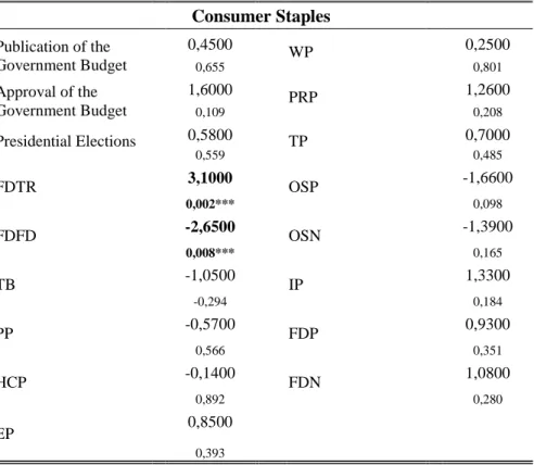
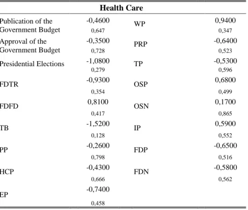
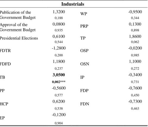
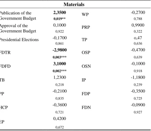
In this section, I perform a second study to further explore the previous results, but now among sectors. I will try to understand if the reactions from sector to sector are different and explain why it happens. The ten sectors which take part of this study are: Consumer Discretionary, Consumer Staples, Energy, Financials, Health Care, Industrials, Information Technology, Materials, Telecommunication Services and Utilities, which results are shown in Tables 5 to 14, respectively.

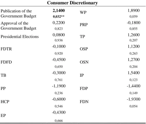
I will begin with the effect of the government budget publication in sector’s returns, since it is the main purpose of this study. Thereby, I can state that only the Consumer Discretionary, Materials and Technology sectors are significantly affected by the President’s budget publication. In the Consumer Discretionary and Materials sectors the budget publication has a positive effect, while in the Technology sector it has a negative effect.

In the Consumer Discretionary sector, which performs better when the economy is doing well, are included retailers, media companies, consumer services companies, consumer durables and apparel companies, and automobiles and components companies. Thereby, there may be a positive reaction of these companies after the budget publication, due to an increase of certainty in the market, which makes it perform better.

The Materials sector is also sensitive to changes in the business cycle. For example, it supplies materials for construction, so it depends on a strong economy. Another factor that influences this sector is the supply and demand fluctuations, where the price of raw materials, such as gold or other metals, is very demand driven. So, the positive effect of a budget publication in this sector is likely due to decisions made by the government in this area, such as gold reserves, which will influence its fluctuation prices. Also decisions like new constructions and projects that will require all kind of raw materials from this area will create a positive effect on this sector, since it is a source of revenues and creation of jobs.

The Technology sector is usually composed by companies that manufacture electronics (computers, stereos, televisions and phones), create software or products, and services related with information technology. In this study, Technology sector is the only negatively affected by the U.S. federal budget publication. This is possibly explained by the way U.S. government spend its money in some sectors, since its investments or disinvestments have a significant impact in the technology sector. Looking at the last few years where the

15

government had considerable cuts, this may be one of the sectors firstly affected, since this is not a primary need for the state.

An expected result in this study is the fact that the budget acceptance does not affect stock market returns, mainly because the market may react in advance to this situation. The market already discounts the effects of this action, so the market returns fluctuations are diluted overtime.

Now I will analyze the effect of the categories expenditures presented in the U.S. federal budget, in each sector. The results are according with what could be expected. There is not a significant impact in sectors’ market returns due to variations in each category expenditure, since it is natural that the way the government spends its money would not affect negatively or positively any sector, because there are no direct expenditures to one specific sector and/or company. In fact, Telecommunication sector was the only one significantly affected by one category of expenditure, Welfare. An increase or decrease over 5% in the Welfare expenditure led to a reduction of stock returns in the Telecommunication sector. It is difficult to explain this result since they are not highly connected with each other. The Telecommunication sector is well known by its high dividend yields and relatively stable cash flows. This sector is usually integrated by telecommunication companies, which commonly are less volatile than the rest of the market and will tend to outperform during an economic crisis.

The main surprise of this study was the fact that the three presidential elections years represented in this study (2004 George W. Bush continued its mandate and 2008 and 2012 Barack Obama was named and continued its mandate as the President of the United States of America, respectively), did not affect the stock returns. This is surprisingly unexpected because the importance of the President by itself is very significant for the U.S. and rest of the World, so the fact of a change in the parties, Bush to Obama, should have had an impact.

The remaining variables to be analyzed are the interest rates. Looking at the variation of U.S. Treasury Bond, which is the fixed-interest U.S. government security with a maturity of ten years, it has a positive effect in the Industrials sector and a negative effect in the Telecommunication and Utilities sectors. The first case, where the Industrials stock returns react well to changes in the U.S. Treasury Bonds, is explained in two different ways. Before the crisis, when the market was performing well, the economy was supporting the results of this sector, since it depends significantly in other companies’ performance, due to its nature.

16

When the crisis started, there was a decrease in the stock prices due to the decrease of economic activity, but there was also a decrease in the Treasury Bonds, since the investors turned to this market due to its low risk. During the crisis, with a low economic growth, the Treasury Bonds rates reduction led the investors to invest in the stocks’ market, increasing its prices, seeking for a return better than a U.S. Treasury Bond. In the second case, the Telecommunications and Utilities sectors’ stocks returns react negatively to changes in the U.S. Treasury Bonds. As explained before, the Telecommunication sector does not suffer like others industries when the economy does not perform well. In the case of the Utilities sector, it is composed by companies that usually carry large amounts of debt, since they have significant infrastructures. With this capital structure, Utilities companies are commonly more sensitive to fluctuations of the interest rates. Logically, this sector will perform better when interest rates are falling or remain low. As interest rates increase or decrease, the debt payments will rise or drop, respectively. Thus, a small increase or an expected increase of the interest rates will negatively affect this sector. Ardagna, S. (2004) stated that when countries improve their fiscal policies, the long-term government bonds decrease and the stock market prices increase, showing that countries with high government deficit like the U.S., that made spending cuts, reduced the interest rates, which led to an increase of the stock market prices.

Now I will analyze the Federal Funds rate, the overnight rate at which the Federal Reserve lends money to financial institutions. This is a reference rate for the market, so its variation is supposed to influence the market and the rest of the interest rates due to its variations or possible variations (expectations). Therefore, it is explained why this rate has a significant impact in 60% of the sectors analyzed in this study. The sectors positively affected are the Telecommunication, Consumer Staples, Technology and Utilities. By the other hand, the sectors negatively affected are the Energy and Materials. Here I am testing the link between monetary policy and stock prices. Makes sense and I can conclude that monetary policy affects stock market prices more than fiscal policy. Afonso and Sousa (2009a) also argued that fiscal policy shocks have a less significant effect in the asset markets of the U.S., being congruent with my previous conclusion above.

Finally, the Financials sector is not influenced by the Federal Funds rate but it is negatively affected by the overnight money market rate. This sector is usually composed by banks, insurance companies and investment funds. It performs better when the interest rates are high, because the margins of mortgages and loans grow.

17 5.3 Event-study Results

In this section I will explore the results of the event-study and robustness test. The past event that I chose in order to apply this methodology is the U.S. President’s budget publication. This is the event surrounding the U.S. federal budget that significantly affected some of the sectors’ stock market returns in the regression. In the event-study, with an event window between [-10, 10], I want to test if this event will affect the sectors significantly affected by this same event in the regression.

In this way, I will use the U.S. federal budget publication as a past event to see how it can affect those sectors, while trying to get a congruent result with the regression. The three sectors studied are: Consumer Discretionary, Materials and Technology. To interpret the impact of U.S. publication on stock returns, I use mainly the abnormal returns on the 10 trading days after and before the budget publication date. The graphs that present the cumulative abnormal returns of these three sectors are represented in Table 15.

Looking at the event-study results for the three sectors analyzed, there are slight differences in the abnormal returns after the budget publication, but not significant enough. This second methodology used does not give the same results as the first methodology did. In some years, and taking into account the graphs from Table 15 and the results in Table 16, there are some budget publications that had a small effect in the returns of these three sectors, but they are not significantly enough to say that there was an effect in stock returns associated with the event U.S. budget publication, possibly explained by an event window too large.

Since in the event window I am including the ten days before the budget publication, I comprise too many expectations in those days, leading to a no significant result in this test. Having this in mind, I decide to run another event study to ensure that I avoid those many expectations in this study, reducing the event window before the event takes place.

The robustness test in the event-study has an event window [-1,10]. Looking at this test, for the three sectors analyzed, only the technology sector is not significantly enough affected by the budget publication. The Consumer Discretionary and Materials sectors are significantly affected by the budget publication. In the Consumer Discretionary, there is evidence in the second and eight days after the budget publication that the results are significantly affected and in the Materials sector, there is evidence in the third day after the budget publication that the results are significantly affected. These results are shown in table 17.

18

6

Conclusion

The main purpose of this study is to answer the following question: how far can the U.S. federal budget affect the stock returns of the S&P 500 sectors indexes? In fact, the relationship between this budget and the stocks returns of the sectors mention above is very important to the U.S. economy. I also state the differences in the results between each sector and why does that happen, since different economic sectors with different characteristics indeed react differently to the same situations.

It is not supposed to see the government budget affecting any specific company, since there is no direct relation between them, i.e., there is no direct spending category that releases money from the government to any specific company. However, the budget publication, acceptance and actions around it should have an impact in some U.S. economic sectors, since this spending shows the directions the government wants to give to its economy, which will influence the environment where companies are operating, thereby affecting its results.

The first and main conclusion is related with the President’s budget publication. This event does not lead to any significant return to S&P 500 index. Looking sector by sector, the President’s budget publication leads to a positive and significant return to the Consumer Discretionary and Materials sectors. On the other hand, it causes a negative and significant return to the Technology sector.

The budget acceptance does not affect stock market returns studied in this study. This is an expected result, since the market may react in advance to this situation. The market already discounts the effects of this action, so its returns fluctuations are diluted overtime. In years of controversial decisions the market is already prepared for them, cushioning its effects on companies. In years of congruent decisions, the market is not significantly affected.

The presidential elections years had no significant effect in stock market returns in this study. The way U.S. government spends its money is represented in each category expenditures of the budget, which also does not affect any sector of the U.S. economy.

Concluding, this dissertation shows how the World’s biggest economy, U.S. economy, is affected by the U.S. federal budget. It states how the President’s budget publication, acceptance and presidential elections years affect stock market returns. It also demonstrates how changes in interest rates have a significant effect in several economic sectors.

19

References

Afonso, A., Sousa, R. M., 2009a. Fiscal policy, Housing and Stock Prices. Working Paper Afonso, A., Sousa, R. M., 2009b. The macroeconomic effects of fiscal policy. Portuguese Economic Journal, 10, 61-82.

Belo, F., Gala, V. D., Li, J., 2011. Government spending, political cycles, and the cross

section of stock returns. Journal of Financial Economics, 107 (2013), 305-324.

Chatziantoniou, I., Duffy, D. and Filis, G. 2013. Stock Market Response to Monetary and

Fiscal Policy Shocks: Multi-Country Evidence. Economic Modelling, 30, 754-769.

Christ, C. F. 1968. A simple macroeconomic model with a government budget restraint. Journal of Political Economy, 76, 53-67.

Coate, S., Morris, S., 1995. On the form of transfers to special interests. Journal of Political Economy, 103, 1210-1235.

Darrat, A. F., 1988. On fiscal policy and the stock market. Journal of Money, Credit and Banking, 20, 353-363.

Don Cram, The Event Study Webpage, Paper

Grenee, W. H., 2008. Econometric analysis. Prentice Hall, 6th edition. Gujarati, D. N., 2004. Basic econometrics. McGraw-Hill, 4th edition. John J. Binder, The Event Study Methodology Since 1969, 111–137 Neves, J. L. C., 2011. Introdução à Economia. Verbo, 9th edition.

Pástor, L., Veronesi, P., 2012. Uncertainty about government policy and stock prices. The Journal of Finance, 67, 1219-1264.

Silvia Ardagna, 2004. Financial Markets’ Behavior Around Episodes Of Large Changes In

The Fiscal Stance. Working Paper, 1-27.

S.P. Kothari, Jerold B. Warner, The Econometrics of Event Studies. Paper Sudi Sudarsanam, Creating Value from Mergers and Acquisitions, Chapter 4

20

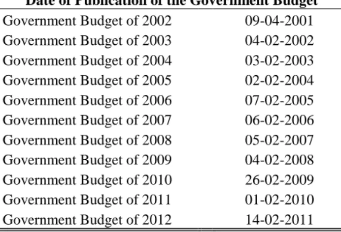
Table 1: Publication and Approval of the Government Budget

Date of Publication of the Government Budget

Government Budget of 2002 09-04-2001 Government Budget of 2003 04-02-2002 Government Budget of 2004 03-02-2003 Government Budget of 2005 02-02-2004 Government Budget of 2006 07-02-2005 Government Budget of 2007 06-02-2006 Government Budget of 2008 05-02-2007 Government Budget of 2009 04-02-2008 Government Budget of 2010 26-02-2009 Government Budget of 2011 01-02-2010 Government Budget of 2012 14-02-2011

Date of Approval of the Government Budget

Government Budget of 2002 24-04-2001 Government Budget of 2003 21-03-2002 Government Budget of 2004 11-04-2003 Government Budget of 2005 20-05-2004 Government Budget of 2006 28-04-2005 Government Budget of 2007 18-05-2006 Government Budget of 2008 13-11-2007 Government Budget of 2009 11-03-2009 Government Budget of 2010 29-04-2009 Government Budget of 2011 09-04-2011 Government Budget of 2012 02-08-2011

21

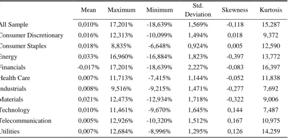
Table 2: Descriptive Statistics of daily returns

This table presents the descriptive statistics results of the all sample study, Consumer Discretionary, Consumer Staples, Energy, Financials, Health Care, Industrials, Materials, technology, telecommunication and utilities sectors. In this test I include descriptive statistics such as mean, maximum and minimum values, standard deviation, skewness and kurtosis on the basis of stock returns. The sample period starts in 2002 and ends in 2012.

Mean Maximum Minimum Std.

Deviation Skewness Kurtosis All Sample 0,010% 17,201% -18,639% 1,569% -0,118 15,287 Consumer Discretionary 0,016% 12,313% -10,099% 1,494% 0,018 9,372 Consumer Staples 0,018% 8,835% -6,648% 0,924% 0,005 12,590 Energy 0,033% 16,960% -16,884% 1,823% -0,397 13,772 Financials -0,017% 17,201% -18,639% 2,227% -0,083 16,397 Health Care 0,007% 11,713% -7,415% 1,144% -0,052 11,838 Industrials 0,008% 9,516% -9,215% 1,471% -0,277 7,692 Materials 0,021% 12,473% -12,934% 1,718% -0,322 9,006 Technology 0,010% 11,461% -9,670% 1,645% 0,144 7,487 Telecommunication 0,005% 12,926% -10,320% 1,512% 0,167 10,975 Utilities 0,007% 12,684% -8,996% 1,295% 0,126 14,259

22

Table 3: Abbreviations

MR Market Return

GBP Government Budget – Publication

GBA Government Budget – Approval

EY Elections Years

FDTR Target Rate - Federal Funds

FDFD Interest Rate - Federal Funds

IRTB Interest Rate - Treasury Bonds

PP Pensions Expenditures

HCP Helath Care Expenditures

EP Energy Expenditures

EN Energy Expenditures (before negative variations)

DP Defense Expenditures

DN Defense Expenditures (before negative variations)

WP Welfare Expenditure

WN Welfare Expenditure (before negative variations)

PRP Protection Expenditures

TP Transportation Expenditures

TN Transportation Expenditures (before negative variations)

GP General Government Expenditures

GN General Government Expenditures (before negative variations)

OP Other Spending Expenditures

ON Other Spending Expenditures (before negative variations)

IP Interest Expenditures

IN Interest Expenditures (before negative variations)

FDP Federal Surplus

FDN Federal Deficit

23

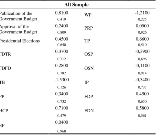
Table 4: All Sample Results

This table presents the all sample results. It includes stock prices of 10 sectors belonging to S&P 500 Index between 2002 and 2012. The Symbols ***, ** and * represent, respectively, the statistical significance at 1%, 5% and 10% significance levels (two-tailed). The sample period starts in October 1 2002 and goes to September 30 2012. The upper number represents the coefficient and the smaller one the p-value, both in the right side of each variable.

All Sample Publication of the Government Budget 0,8100 _WP -1,2100 0,419 0,225 Approval of the Government Budget 0,2400 _PRP 0,0900 0,809 0,926 _{Presidential Elections} 0,4500 _TP 0,6600 0,650 0,510 FDTR 0,3700 OSP -0,3900 0,712 0,696 FDFD 0,2800 OSN -0,1100 0,782 0,914 TB -1,5300 IP -0,3400 0,126 0,737 PP 0,3400 FDP 0,4500 0,732 0,650 HCP 0,7100 FDN 0,5800 0,479 0,561 EP 0,0400 0,968

24

Table 5: Consumer Discretionary

This table presents the consumer discretionary sector. It includes stock prices of 10 sectors belonging to S&P 500 Index between 2002 and 2012. The Symbols ***, ** and * represent, respectively, the statistical significance at 1%, 5% and 10% significance levels (two-tailed). The sample period starts in October 1 2002 and goes to September 30 2012. The upper number represents the coefficient and the smaller one the p-value, both in the right side of each variable. Consumer Discretionary Publication of the Government Budget 2,1400 _WP 1,8900 0,032** 0,059 Approval of the Government Budget 0,2200 PRP -0,1800 0,823 0,855 _{Presidential Elections} 0,0800 _TP 1,2600 0,936 0,207 FDTR -0,1000 OSP 1,1200 0,920 0,263 FDFD -0,4500 OSN 1,2700 0,650 0,204 TB -0,3000 IP 1,5400 0,761 0,123 PP -1,1900 FDP -1,4400 0,236 0,149 HCP -0,6000 FDN -1,9300 0,546 0,054 EP -0,4300 0,666

25

Table 6: Consumer Staples

This table presents the consumer staples sector. It includes stock prices of 10 sectors belonging to S&P 500 Index between 2002 and 2012. The Symbols ***, ** and * represent, respectively, the statistical significance at 1%, 5% and 10% significance levels (two-tailed). The sample period starts in October 1 2002 and goes to September 30 2012. The upper number represents the coefficient and the smaller one the p-value, both in the right side of each variable. Consumer Staples Publication of the Government Budget 0,4500 _WP 0,2500 0,655 0,801 Approval of the Government Budget 1,6000 _PRP 1,2600 0,109 0,208 _{Presidential Elections} 0,5800 _TP 0,7000 0,559 0,485 FDTR 3,1000 OSP -1,6600 0,002*** 0,098 FDFD -2,6500 OSN -1,3900 0,008*** 0,165 TB -1,0500 IP 1,3300 -0,294 0,184 PP -0,5700 FDP 0,9300 0,566 0,351 HCP -0,1400 FDN 1,0800 0,892 0,280 EP 0,8500 0,393

26 Table 7: Energy

This table presents the consumer energy sector. It includes stock prices of 10 sectors belonging to S&P 500 Index between 2002 and 2012. The Symbols ***, ** and * represent, respectively, the statistical significance at 1%, 5% and 10% significance levels (two-tailed). The sample period starts in October 1 2002 and goes to September 30 2012. The upper number represents the coefficient and the smaller one the p-value, both in the right side of each variable. Energy Publication of the Government Budget 1,1600 _WP -1,6300 0,247 0,102 Approval of the Government Budget -1,4000 _PRP 0,8600 0,161 0,387 _{Presidential Elections} 0,5000 _TP -0,3500 0,618 0,725 FDTR -3,1100 OSP -1,0900 0,002*** 0,274 FDFD 3,6000 OSN -0,8900 0,000*** 0,037 TB 1,6800 IP -1,1900 0,093 0,233 PP 0,0800 FDP 1,0600 0,934 0,290 HCP 1,4700 FDN 1,6600 0,140 0,097 EP 0,4500 0,650

27

Table 8: Financials

This table presents the Financials sector. It includes stock prices of 10 sectors belonging to S&P 500 Index between 2002 and 2012. The Symbols ***, ** and * represent, respectively, the statistical significance at 1%, 5% and 10% significance levels (two-tailed). The sample period starts in October 1 2002 and goes to September 30 2012. The upper number represents the coefficient and the smaller one the p-value, both in the right side of each variable.

Financials Publication of the Government Budget 0,7700 _WP 1,0200 0,442 0,306 Approval of the Government Budget 0,8100 _PRP 0,1900 0,418 0,849 _{Presidential Elections} -0,6200 _TP -0,4300 0,534 0,669 FDTR 1,5200 OSP 0,4500 0,128 0,655 FDFD -2,7600 OSN 0,5400 0,006*** 0,591 TB -1,2100 IP -1,3300 0,225 0,185 PP -0,8200 FDP -1,4100 0,410 0,158 HCP -0,5000 FDN -1,2800 0,616 0,199 EP -0,000 0,999

28

Table 9: Health Care

This table presents the Health Care sector. It includes stock prices of 10 sectors belonging to S&P 500 Index between 2002 and 2012. The Symbols ***, ** and * represent, respectively, the statistical significance at 1%, 5% and 10% significance levels (two-tailed). The sample period starts in October 1 2002 and goes to September 30 2012. The upper number represents the coefficient and the smaller one the p-value, both in the right side of each variable.

Health Care Publication of the Government Budget -0,4600 _WP 0,9400 0,647 0,347 Approval of the Government Budget -0,3500 _PRP -0,6400 0,728 0,523 Presidential Elections -1,0800 TP -0,5300 0,279 0,596 FDTR -0,9300 OSP 0,6800 0,354 0,499 FDFD 0,8100 OSN 0,1700 0,417 0,865 TB -1,5200 IP 0,5900 0,128 0,552 PP -0,2600 FDP -0,6500 0,798 0,516 HCP -0,4300 FDN -0,5800 0,666 0,562 EP -0,7400 0,458

29

Table 10: Industrials

This table presents the Industrials sector. It includes stock prices of 10 sectors belonging to S&P 500 Index between 2002 and 2012. The Symbols ***, ** and * represent, respectively, the statistical significance at 1%, 5% and 10% significance levels (two-tailed). The sample period starts in October 1 2002 and goes to September 30 2012. The upper number represents the coefficient and the smaller one the p-value, both in the right side of each variable.

Industrials Publication of the Government Budget 1,3200 _WP -0,9500 0,188 0,344 Approval of the Government Budget 0,0800 _PRP 0,1300 0,935 0,898 _{Presidential Elections} 0,6100 _TP 1,8600 0,544 0,062 FDTR -1,2800 OSP -0,0200 0,200 0,985 FDFD 1,1800 OSN 1,1000 0,237 0,272 TB 3,0500 IP -0,3400 0,002*** 0,731 PP -0,5600 FDP -0,7600 0,577 0,450 HCP 0,6200 FDN -0,7300 0,538 0,463 EP -0,1200 0,904

30

Table 11: Materials

This table presents the Materials sector. It includes stock prices of 10 sectors belonging to S&P 500 Index between 2002 and 2012. The Symbols ***, ** and * represent, respectively, the statistical significance at 1%, 5% and 10% significance levels (two-tailed). The sample period starts in October 1 2002 and goes to September 30 2012. The upper number represents the coefficient and the smaller one the p-value, both in the right side of each variable.

Materials Publication of the Government Budget 2,3500 _WP -0,2700 0,019** 0,788 Approval of the Government Budget 0,1000 _PRP 0,9900 0,922 0,322

_{Presidential Elections} -0,1700 _TP o,47

0,861 0,636 FDTR -2,9800 OSP -0,4700 0,003*** 0,639 FDFD 3,1000 OSN -0,1000 0,002*** 0,918 TB 1,2300 IP -1,1800 0,218 0,239 PP -0,2100 FDP -0,3500 0,835 0,725 HCP -0,3600 FDN -0,0900 0,721 0,927 EP 0,4200 0,672

31

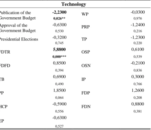
Table 12: Technology

This table presents the Technology sector. It includes stock prices of 10 sectors belonging to S&P 500 Index between 2002 and 2012. The Symbols ***, ** and * represent, respectively, the statistical significance at 1%, 5% and 10% significance levels (two-tailed). The sample period starts in October 1 2002 and goes to September 30 2012. The upper number represents the coefficient and the smaller one the p-value, both in the right side of each variable.

Technology Publication of the Government Budget -2,2300 _WP -0,0300 0,026** 0,976 Approval of the Government Budget -0,6300 _PRP -1,2400 0,530 0,216 _{Presidential Elections} -0,3200 _TP -1,2300 0,745 0,220 FDTR 5,8800 OSP 0,6100 0,000*** 0,539 FDFD 0,8500 OSN -0,2100 0,394 0,836 TB 0,6900 IP 0,3000 0,490 0,766 PP 1,8500 FDP 1,2600 0,064 0,208 HCP -0,5900 FDN 0,8800 0,556 0,381 EP -0,6300 0,527

32

Table 13: Telecommunication

This table presents the Telecommunication sector. It includes stock prices of 10 sectors belonging to S&P 500 Index between 2002 and 2012. The Symbols ***, ** and * represent, respectively, the statistical significance at 1%, 5% and 10% significance levels (two-tailed). The sample period starts in October 1 2002 and goes to September 30 2012. The upper number represents the coefficient and the smaller one the p-value, both in the right side of each variable. Telecommunication Publication of the Government Budget -0,8200 _WP -2,0600 0,411 0,039** Approval of the Government Budget -0,6600 _PRP -0,3000 0,511 0,767 _{Presidential Elections} 1,0200 _TP 1,6000 0,308 0,110 FDTR 2,0700 OSP -0,2700 0,037** 0,785 FDFD -0,6600 OSN -0,0600 0,506 0,956 TB -3,4900 IP 0,8400 0,000*** 0,399 PP 1,7400 FDP 1,2700 0,082 0,203 HCP 0,0800 FDN 0,4900 0,939 0,621 EP 0,3400 0,734