Option pricing under jump-diffusion models

(1)

INSTITUTO SUPERIOR DAS CIÊNCIAS, DO TRABALHO E DA EMPRESA DEPARTAMENTO DE FINANÇAS

UNIVERSIDADE DE LISBOA FACULDADE DE CIÊNCIAS DEPARTAMENTO DE MATEMÁTICA

Option Pricing under jump-diffusion models

Ricardo Filipe Machado Venâncio

!

Mestrado em Matemática Financeira

Dissertação orientada por:

João Pedro Vidal Nunes

(2)

Acknowledgments

This thesis is the final result after enrolling in the Master of Mathematics applied to Finance. It lead me to achieve great knowledge about Finance, particularly on how to approach the question of computing a fair value for financial contracts.

In first place, I thank to all the students and professors I had contact with in FCT-UNL, where I got my bachelor’s degree in Mathematics. Long were the hours I spent in teachers’ offices clarifying my doubts which were promptly and enthusiastically answered. Their patience and dedication on my and my colleagues formation was crucial to become the person I am today.

In second place, I thank my supervisor, João Nunes, who patiently taught me the main topics related to the Pricing theory and who helped me with many questions I had, without any hesitation. He gave me important tools so that I could design the work I am presenting here and without which I could not develop this dissertation.

I also appreciate the help of all the people who I worked with in BNP Paribas, who encouraged me during my learning process while I was working as an intern. They pro-posed me challenges and pro-posed questions who helped me to better understand how Fi-nancial markets work and contributed to my professional and personal growth. Thanks to this working experience, I was able to establish a link between what is developed in theory and relate it to the practice.

Finally, I thank my family for all the support, specially in the moments I was absent living and working abroad.

I hope the work I developed is useful for who studies matters related to Option Pricing and the reader find it interesting to explore.

(3)

Resumo

Nesta tese, apresentam-se métodos para resolver numericamente equações diferen-ciais por forma a obter preços de contractos financeiros. Em particular, dá-se ênfase a opções vanilla de estilo europeu e americano cujo activo subjacente segue um modelo de difusão com saltos. Quanto à distribuição destes útltimos, destacam-se o modelo de Merton, que considera que eles têm uma distribuição Normal, e o de Kou, onde é assum-ida uma dupla distribuição exponencial. Este tipo de modelos representa uma extensão dos clássicos modelos de difusão, como o famoso modelo de Black-Scholes-Merton, e tem como objectivo superar algumas das falhas inerentes a este último, tal como cau-das muito curtas e picos baixos da distribuição do logaritmo dos retornos do activo, que não reflectem, em geral, o sentimento dos investores nos mercados financeiros, aliando, ao mesmo tempo, a simplicidade e eficiência dos modelos de difusão.

Para alcançar o nosso objectivo, estabelece-se inicialmente qual é a equação que de-screve a dinâmica do valor dos preços das opções referidas em relação a vários parâmet-ros, tal como o valor do preço do activo subjacente e o tempo até à maturidade. Em seguida, constróem-se partições para a resolução numérica do problema, através da dis-cretização da função que descreve o preço do contracto financeiro por diferenças finitas. Esta abordagem é útil visto que permite obter preços de contractos cujo "payoff" não é tão simples quanto o de opções vanilla e para os quais não existem fórmulas fechadas ou semi-fechadas para o seu valor em cada momento do tempo até à sua maturidade.

No final, expõem-se os resultados encontrados para diferentes resoluções das par-tições, comparados com referências da literatura, e apresentam-se algumas conclusões.

(4)

Abstract

In this dissertation, methods to solve numerically partial differential equations in order to obtain prices for contingent claims are presented. In particular, we highlight European and American style vanilla options, whose underlying asset follows a jump-diffusion model. For the distribution of the jumps, the Merton and Kou models are studied. The former considers these have a Normal distribution, whereas the latter assumes a double-exponential. These type of models represent an extension of the classic diffusion models, such as the famous Black-Scholes-Merton, and has the goal of overcoming its flaws, such as thin tails and low peaks in the distribution of the logarithm of the asset returns, that do not reflect the general investors sentiment in the financial markets, while maintaining the simplicity and tractability inherent to diffusion models. To accomplish our goal, an equation describing the relation of the value of the referred options on several parameters, such as the time-to-maturity and the spot value of the underlying asset is suggested. We then build partitions in order to numerically solve our problem using finite differences, discretizing the function which provides the price of our contingent claim. This approach is useful, since it allows to obtain prices of contracts whose payoff is not as simple as the vanilla options’ and for which it does not exist closed or semi-closed formulae for its value at each point in time until maturity.

Finally, we expose results found for each one of partitions considered, comparing them with values in the literature, and some conclusions are presented.

(5)

Keywords

Option Pricing Lévy processes Diffusion models Jump-diffusion models European Options American Options LU decomposition Tridiagonal matrices Numerical discretization Finite differences

(6)

1

Introduction

Although options were created a long time ago, it was only on the 26th April 1973 that the Chicago Board Options Exchange (CBOE) traded the first listed option. Since then, interest in options has excessively grown from only 911 contracts on 16 underlying stocks to millions of contracts with total notional value of several trillion dollars in CBOE and in other stock exchanges around the world.

An option, as the name itself indicates, gives to its holder the right to buy or sell an asset, but not the obligation to do so, unlike other contracts such as futures or forwards. To compensate for this benefit, the holder of the option must pay an up-front fee, called the "premium". The most basic existing options are vanilla calls and puts. Call options give the entity that hold them the right to buy a determined amount of an asset at or until a specified time in the future, defined as the "expiration date" or "maturity date", for a pre-specified price, which we name as the "strike price". Puts, on the other hand, permit the entity to sell the asset. The asset in question, in this instance, can be a simple stock, index, bond or a basket composed of several securities.

Based on the time at which options can be exercised, they can be divided into two categories: European or American options. The former gives the right to its owner to exercise the option at the maturity date T , whereas the latter can be exercised at any time until T .

Let us assume the underlying asset is a stock with price S, using St as notation for

its value at time t, prior to T . In the case of a call option, at maturity, it will only be exercised if ST > K, with K being the strike price, whereas otherwise it will expire

(10)

valuing zero. In the case of a put option, the logic is similar, but this contract will only have non-null value if ST < K.

Like any other contingent claim, options are attractive, because they are highly useful in hedging and for speculation. Hedging refers to the act of using financial instruments to cover the position a market agent has in its portfolio in order to avoid big losses, in other words, reducing risk. As a simple example, a put option may be a good instrument to acquire if one is afraid that the price of a certain stock will fall. This way, a minimum selling price is guaranteed (the strike) and the risk of a loss is minimized.

These kinds of financial products obviously require a price to be quoted in the market. And since nobody has a crystal ball, that reveals what happens to an asset’s future price, mathematical models are needed to compute their fair-value. To this end, the work carried out by Robert Merton, Fisher Black and Myron Scholes is of greater importance. They developed a set of formulae based on the Brownian motion which allow us to price many financial derivatives such as calls, puts and barrier options [10]. The Black-Scholes-Merton (BSM) model tries to replicate the dynamics of a financial asset through a geometric Brownian motion, i.e., for a given moment in time t, the expression that gives an asset’s price is St= S0eµt+‡Wt and the continuous compounded

return, ln(St/S0), has a normal distribution. Here, {Wt, t Ø 0} is a Brownian motion,

which has a normal distribution with mean 0 and variance t, µ is called the drift, which measures the annualized average return, ‡ is called the volatility, which corresponds to the annualized standard deviation of the underlying asset price return, S0 is the initial

stock price and "ln" represents the Neperian logarithm.

However, take a look at Figure A.1, in the Appendix. In this figure, you can visualize Standard & Poor’s 500 (S&P500 for short) prices through the year of 2015. This is a very liquid American stock market index based on the market capitalization of 500 large companies that have their common stock listed on the NYSE (New York Stock Exchange) or NASDAQ (National Association of Securities Dealer Automated Quotation system). As you can see by the first chart, there seems to be a large fall in the

(11)

S&P index price towards the end of August 2015. This is highlighted by the computation of log returns (defined as the continuously compounded returns) and represented in Figure A.2. A.2 also reveals a peak at the end of August. This was due to a fall in China’s stock market, which at that time affected the U.S.’ markets. On the other hand, Figure A.5, which represents a histogram of the log returns of the S&P, reveals some interesting characteristics: an asymmetric feature, a higher peak and two heavier tails than those of the normal distribution. To illustrate this idea, in this same figure, a normal distribution with the same mean and standard deviation as the price series is plotted in red to compare.

As another example, in January 2015, the Swiss National Bank (SNB) discontinued the minimum EUR/CHF exchange rate, which was fixed with a floor of 1.20 since 2011. This measure taken by the SNB, provoked a huge fluctuation of this rate which is illustrated by Figures A.3 and A.4. These charts, such as in the previous example, stand respectively for the values of the EUR/CHF in 2015 and the corresponding log returns. Looking into the histogram A.6, it is also evident that the log-returns of the underlying are not normally distributed. To sustain this idea, we first present two definitions:

Definition 1.1. Given a random variable X, the kurtosis and skewness of X are

re-spectively defined as E[(X≠µ

‡ )3] and E[( X≠µ

‡ )4], where E(·) is the expected value of the

random variable X.

The price series corresponding to the S&P500 presents a skewness equal to -1.2752 and kurtosis equal to 4.1427. The EUR/CHF log returns have these values respectively equal to 1.8168 and 8.5888. Comparing to the normal distribution, which has a skewness of zero and kurtosis equal to 3, we see that for both series, the values are far from normal. Moreover, we see that these series are "leptokurtic", meaning their kurtosis is above 3. A Jarque-Bera (see [7] for more details) test was performed to evaluate the normality of the presented series. This test has as null hypothesis that the sample data of a random variable comes from a normal distribution. The alternative hypothesis is that it does not. With a confidence level of 95%, the null hypothesis was rejected, which means the

(12)

assumption of a normal distribution for the log-returns of these assets is not plausible. This is even more evident if we look into the histogram of S&P500 because it displays a high peak and asymmetric heavy tails. These characteristics are not exclusive for this index and are also present for almost all financial asset prices like individual stocks, foreign exchange rates and interest rates.

Therefore, as you can observe, the normal distribution does not fit very well with empirical data, since the empirical distribution of asset returns exhibits fat tails and skewness, a behaviour that deviates from normality and is inconsistent with the BSM model. Besides, as also evident in the images referred before, asset price processes have jumps or spikes and must be taken into account when pricing financial contingent claims. This is crucial for the estimation of current market values of portfolios held by companies that deal on a daily basis with products that depend on financial assets, such as banks and hedge funds. More importantly, it is essential to provide prices of contingent claims to clients who take into account these events.

It is then evident that under the geometric Brownian motion variations of great amplitude are not likely to happen as it assumes the log-returns have a normal distri-bution. This is documented with empirical evidence in [30]. Besides, Brownian motion is almost surely continuous by definition, a feature that is inconsistent with the exis-tence of referred variations, which are commonly called "jumps" in literature. One way to try to get around the problem is to consider Lévy processes in which non-marginal variations are more likely to happen as a consequence of fat-tailed distributions based processes. Lévy based models are therefore much more realistic.

On the other hand an essential requirement for using a pricing model, independently of the considered distribution for the asset returns, is that it should ensure that the prices of actively traded instruments such as Europeans options coincide as much as possible with their market price. However, despite its excellent analytical tractability, this condition is not fulfilled in the case of the BSM model. The BSM model does not track the market’s implied volatility well enough. In fact, by inverting the BSM formula with respect to the volatility for a series of options with different strikes and

(13)

with the same maturity, one should obtain approximately the same (constant) implied volatility. However, it is an empirical fact that the graph of the implied volatility is not a horizontal line as a function of strike or as a function of time to maturity, but resembles a "smile" instead, as reported by Hull [29]. Thus, using a single value for the volatility in order to price options with different strikes and maturities leads us to get prices that are not in accordance with the ones displayed in the financial markets.

It then makes sense to consider an alternative for the BSM model. Jump-diffusion models and Lévy based models, proposed in the late 1980s and early 1990s, are attrac-tive because they explain the jump patterns exhibited by some stocks. Studies reveal that Lévy models are realistic when pricing options close to maturity [14]. However, they are more difficult to handle numerically. And in contrast to the basic BSM model, Lévy models do not immediately make obvious which hedging strategy leads to an instantaneous risk-free portfolio.

The aim of this thesis is then to introduce the Lévy processes and models based on these in order to incorporate the features discussed above and try to overcome some of the flaws in the BSM model. It is important to come up with a pricing model that traders and other market agents can utilize that captures the behavior of implied volatility smiles more accurately and considers the occurrence of jumps in order to handle the risks of trading. Lévy processes provide us with appropriate tools to adequately and consistently describe all these observations, both in the ‘real’ and in the ‘risk-neutral’ world as we shall see through the rest of this thesis.

The main idea is to replace the Normal distribution of the increments by a more general distribution that is able to better reflect the stylized facts such as the skewness and excess kurtosis present in the financial markets. Examples of distributions that attempt to achieve this are the Variance Gamma [40], the Normal Inverse Gaussian [4], the CGMY [11] and the Hyperbolic Model [18]. These admit the possible existence of an infinite number of jumps in any interval and so are called "infinite activity models". Here, the price behavior on small time intervals is modeled by jumps and the Brownian motion is no longer needed. We will, however, deal only with jump diffusions. For a

(14)

more interested reader in infinite activity models, we suggest the consultation of [14], [42] or [44]. Pure jump models with finite activity are also possible but, according to [14], they do not lead to a realistic description of price dynamics.

In defiance of the analytical tractability offered by the Lévy processes, the con-straints of independence and stationarity of their increments bring some drawbacks. Mandelbrot and Hudson [30] advocate Lévy processes lead to rigid scaling properties for marginal distributions of returns which are not observed in empirical time series. On the other hand, in spite of being able to calibrate the implied volatility patterns for a single maturity under the risk neutral measure, they fail to reproduce correct option prices over a range of different maturities. Both issues are owed to the fact that expo-nential Lévy models do not allow for time inhomogeneity. It has been observed that the estimated volatilities change stochastically over time and are clustered as reported in [14] or [30].

Local volatility models were proposed as an alternative. For example, Cox [16] intro-duced the Constant Elasticity Variance (CEV) model which attempted to introduce the leverage effect. It tries to incorporate the fact that in equity markets volatility increases when prices decrease due to investors fear sentiment. The opposite effect occurs in com-modity markets. Heston [28] considered a diffusion-based stochastic volatility model in which the price and volatility are correlated and the latter follows a squared-root process.

A jump-diffusion stochastic volatility model was proposed by Bates in [5], which deals with this problem by adding proportional log-normal jumps to the Heston stochas-tic volatility model.

Despite the flaws inherent in Lévy processes, they are very useful for pricing purposes and provide an analytical tractability that more sophisticated models do not. In this thesis we start by presenting some theory on the important concepts related to Lévy processes in Chapter 2 and then introduce two models in Chapter 3, one which dates back to Merton [41] and considers that the logarithm of the asset price returns follows a diffusion with jumps that have a normal distribution and a more recent one, developed

(15)

by Kou [33] where it is assumed that jump sizes have a double exponential distribution. Presented these two jump-diffusion models, we explain, in Chapter 4, the rationale behind the fact that assuming assets are driven by Lévy processes leads to the existence of markets which are not complete. We establish the existence of a partial integro-differential equation (PIDE) using a risk-free measure in Chapter 5, that describes the dynamics of the price of a European put option under the jump-diffusion model. Chapter 6, provides a localization error estimate using the asymptotic behavior of the European put option and Chapter 7 explains how to construct the implicit method by using three time levels.

One can apply several numerical tools to calculate option prices such as Monte Carlo simulation and finite-difference methods or use numerical integration techniques when the closed-form solution of the characteristic function of the log returns is known.

Monte Carlo simulation in its most basic form is probably the simplest numerical method one can implement (see [26] for more details). As long as American features are not required and great accuracy is not necessary, Monte Carlo is a very good method for pricing options. However, these methods may take considerable time to simulate.

The purpose of this dissertation is to develop a finite difference method which avoids iteration at each time step and has a second-order convergence rate to solve the PIDE under the jump-diffusion model. Almendral and Oosterlee [1] suggested finite difference and element methods with the second-order backward differentiation formula (BDF2) in the time variable for pricing European options under the jump-diffusion model. These implicit methods with the BDF2 use iterative techniques to solve linear systems in-volving dense matrices and implement the FFT for the integral term to reduce the computational complexity. The numerical method in [15] uses two time levels but only has a first-order convergence rate without iteration at each time step. Another numer-ical method in [22] also uses two time levels according to the Crank-Nicolson scheme and has the second-order convergence rate. However, it must carry out iterations at each time step. For this reason, it is necessary to use three time levels. We particularly focus on the construction of linear systems whose coefficient matrices are not dense but

(16)

tridiagonal matrices instead. So the implicit method can be solved easily by using LU decomposition.

Regarding American-style options, Forsyth-Labahn [23] and d’Halluin-Forsyth-Vetzal [22] proposed an implicit method of the Crank–Nicolson type combined with a penalty method for pricing American options under the Merton model. In [23] the authors showed that the fixed point iteration at each time step converges to the solution of a linear system of discrete penalized equations. In the case of American options under the Kou model, Toivanen [51] developed numerical methods coupled with two alternative ways to solve the LCPs. One is the operator splitting method introduced by Ikonen and Toivanen [31], and the other is the penalty method proposed by d’Halluin, Forsyth, and Labahn [23]. These numerical methods use iterative techniques to solve linear systems involving dense coefficient matrices.

We provide results in Chapter 8 that show our method is stable and consistent with respect to the discrete l2_{-norm in the sense of the Von Neumann analysis and prove it}

has second-order convergence rate.

Chapter 9, presents the numerical results we obtain for vanilla European options for the implicit method with three time levels under the Merton and Kou models. Chapters 10, 11 and 12 represent an extension of the European options to options with American-style features where theory related to this kind of contracts is described as along with the results for the numerical tests performed.

(17)

2

Lévy processes

Before defining a Lévy process, a few concepts are introduced which are useful to comprehend what follows next. For a better understanding or a more detailed study, the reading of [32] or [39] is suggested.

Definition 2.1. A stochastic process is a mathematical model for the occurrence, at

each moment after an initial time, of a random phenomenon. The randomness is captured by the introduction of a measurable space called the sample space, on which probability measures can be placed. From now on, we define as the probability space, the set which contains all the possible events. Thus, a stochastic process is a collec-tion of random variables (Xt)_t_œR+ on ( , F), which take values in a second measurable space ( Õ_,_FÕ), called the state space. F and FÕ represent sigma-algebras and in this

framework, the state space will be the d-dimensional Euclidean space equipped with the sigma-field of the Borel sets. The index t œ [0, +Œ) of the random variables X is interpreted as the time.

Definition 2.2. A filtration in a measurable space ( , F) is a family of sub-‡-algebras

of F, (Ft)_t_œI, with I being a set of indexes, such that if 0 Æ s Æ sÕ then Fs µ FsÕ.

The ‡-algebra Ft represents the information we have at time t. When, for each

t _{Ø 0, the random variable X}t is Ft-measurable, we say that the process (Xt)_t_œR+₀ is

adapted to (Ft)tœI.

Within all the results that will be presented from now on, the following hypotheses shall be implicitly assumed:

(18)

• It is possible for short-sales to take place, i.e., we can sell an asset which we do not possess;

• The asset’s quantities we are trading may not be integer values, they may be any real number;

• The price for selling a security is the same as the price for buying the same security;

• There are no transacting costs;

• The market is completely liquid, meaning that it is always possible to buy or sell any asset we want.

These hypothesis are not precisely verified in real life, but they allow for a conve-nient simplification of our models. Moreover, we shall also suppose that no arbitrage opportunities exist. This will be important for pricing derivative products using a "risk-neutral measure". In a nutshell, an arbitrage opportunity is a way to obtain profits, without an initial investment and without any risk. In general, when those appear in the market, they quickly vanish, returning the assets’ prices to their "equilibrium value" and that is why they are assumed to be nonexistent.

Definition 2.3. Suppose ( , F, P) is a probability space, where is the set containing

all the possible events, F a ‡ ≠ algebra and P a probability measure, often mentioned as the "physical measure" in the literature.

A one-dimensional stochastic process {Lt}tØ0 on a probability space ( , F, P) is a

Lévy process if (see [43]): (1) L0 = 0 almost surely (a.s.);

(2) It has independent increments, that is, for any 0 Æ s < t < s’< t’ the random variables Lt - Ls and LtÕ - L_sÕ are independent;

(3) It has stationary increments, that is, for any 0 Æ s Æ t Æ Œ the law of Lt - Ls

(19)

(4) It is stochastically continuous, that is, lim

tæ0P(|Ls+t ≠ Ls| Ø ‘) = 0, ’‘ Ø 0;

(5) The sample paths are right continuous with left limits a.s.

Examples of Lévy processes are the Brownian motion, the Poisson processes and also its extension to a Compound Poisson Process. These processes are defined and some of their properties are described in the Appendix.

From the definition, we can deduce that the value of a Lévy process in a certain point in time does not depend on its past values, i.e., it evolves independently of what happened before that time instant. Besides, if we look into a specific time interval, that is, to an increment from one point to another with a determined length, the distribution of the difference between the variable in the last point and the one at the first point is the same as the distribution of an increment with the same length, but considering other two moments in time. This may be a flaw when applying to reality, but from an application point of view, it is a simplification which will make the pricing model we are introducing in the next chapters much simpler to analyse. To illustrate this idea, imagine, for instance, that we are modelling the number of cars who cross a certain bridge in one day. Usually, the number of cars who cross it between 2 and 3 pm is much less than the number who pass between 8 am and 9 am or between 6 pm and 7 pm, because the latter usually is the rush hour. Therefore, it might not be suitable that the distribution in the rush hour is the same as the one between 2 and 3 pm.

2.1 Geometric Lévy processes

Once we define a Lévy process, we can model the asset value by what we call the geometric Lévy process, St = S0eLt, on the filtered probability space ( , F, Ft,P),

where Ftis the filtration generated by the Lévy process {Lt}tØ0. This process somehow

represents an extension to the geometric Brownian motion (GBM). The GBM is the solution of the stochastic differential equation

dSt

St

(20)

and, as we shall see, the geometric Lévy process (GLP) follows a similar dynamic, but with an added jump component. Here, µ stands for the mean of the asset’s return and

‡ its annualised volatility.

The GBM is a case of a diffusion process, which assumes no jumps take place, contrasting with jump-diffusion processes.

Definition 2.4. A pure jump process (Jt)tØ0 is constant between jumps and is adapted

and right-continuous.

As an example, Figure (A.7) in Appendix illustrates a simulation of a Poisson pro-cess, which is a particular case of a pure jump process. The expected number of events per unit time was set to 0.1. The horizontal axis represents time and the vertical the value of the random variable, denoted by N(t).

When we combine diffusion processes with pure jump ones, we create what is defined as a jump-diffusion process:

Definition 2.5. A jump-diffusion or jump process is a process of the form

Xt= X0+ ⁄ t 0 “sdWs+ ⁄ t 0 ◊sds+ Jt := XC t + Jt,

where (Jt)tØ0 is a pure jump process and XtC is the continuous part of Xt. (“s)sØ0 and

(◊s)sØ0 are adapted processes and (Ws)sØ0 is a Brownian motion.

As with most of density distributions, it is often useful to know what is the respec-tive characteristic function. The next very useful theorem, commonly referred as the Lévy–Khintchine representation, allows the description of the characteristic function of the large family of Lévy-process and despite being very technical, its proof can be found in [49].

(21)

2.2 Lévy–Khintchine representation

Theorem 2.6. Let (Lt)tØ0 be a Lévy process. For all z œ R and t Ø 0,

E(eizLt) = exp

S Ut Q a_≠a 2z2+ ibz + ⁄ R (eizx_{≠ 1 ≠ izx11} |x|Æ1)d‹(x) R b T V, (2.2)

where a is a non-negative real number, b is a real number and ‹ is a measure on R satisfying ‹{0} = 0 and ⁄

R

min(1, x2_{) d‹(x) < Œ.}

The set of three parameters (a, b, ‹) is commonly known as the generating Lévy triplet. The first parameter a is called Gaussian variance, since it is associated with the Brownian part of the Lévy process and the third quantity ‹ is called Lévy measure. If

‹ = 0 then Lt is a drifted Brownian motion and if a = 0 then Lt is said to be purely

non-Gaussian.

From the definition of a Lévy process, we know that the sample paths are càdlag ("continue à droite, limité à gauche"), over finite intervals [0, t], t Æ T, i.e., they are right-continuous and have left limits almost surely. Thus, any path has only a finite number of jumps with absolute jump size larger than ‘ for any ‘ > 0. As a consequence, the sum of jumps along [0, t] with absolute jump size bigger than 1 is a finite sum for each path. Of course instead of the threshold 1, one could use any number ‘ > 0 here. Contrary to the sum of the big jumps, the sum of the small jumps does not converge in general. There might be too many small jumps to get convergence. This is the reason why we need the term izx11|x|Æ1 in equation (2.2) in general, so that the

integral converges. However, according to Sato [49], it is necessary a Lévy measure satisfies⁄

R

(|x| · 1)‹(dx) < Œ, (this means that the jump part of the Lévy process is of finite variation), in order for the truncation of small jumps not to be needed in (2.2). The symbol · stands for the minimum between two quantities (in this case, |x| and 1). Furthermore, if the Lévy density decays fast enough as x æ ±Œ, we can replace

izx11_|x|Æ1 by izx. If the process is of finite variation, then we do not need this term at

all.

(22)

activity. In the former case, the aggregate jump arrival rate is finite, whereas in the latter case, an infinite number of jumps can occur in any finite time interval. Within the infinite activity category, the sample path of the jump process can either exhibit finite variation or infinite variation. In the former case, the aggregate absolute distance travelled by the process is finite, while in the latter case, the aggregate absolute distance travelled by the process is infinite over any finite time interval.

‹(dx) is interpreted as the expected number of jumps per unit of time whose size

belongs to the set dx. Therefore, we formally summarize the last paragraphs in the following two results, found in [49]:

Theorem 2.7. Let Lt be a Lévy process with triplet (a, b, ‹).

(1) If ‹(R) < Œ, then almost all paths of Lt have a finite number of jumps on every

compact interval. The Lévy process has finite activity.

(2) If ‹(R) = Œ, then almost all paths of Lt have an infinite number of jumps on

every compact interval. The Lévy process has infinite activity.

Theorem 2.8. Let Lt be a Lévy process with triplet (a, b, ‹).

(1) If ‡2 _{= 0 and} ⁄ R

(|x| · 1)‹(dx) < Œ, then almost all paths of Lt have finite

variation.

(2) If ‡2 _{”= 0 or} ⁄ R

(|x| · 1)‹(dx) = Œ, then almost all paths of Lt have infinite

variation.

For the particular case of a compound Poisson process, only a finite number of jumps in any finite time interval take place, meaning the truncation function in (2.2) can be omitted when deriving the characteristic function of this process.

(23)

2.3 Drifted Brownian motion with a finite number

of jumps

Consider the following process, corresponding to the drifted Brownian motion with a finite number of jumps:

Lt= A µ_≠ ‡ 2 2 B t+ ‡Wt+ Nt ÿ i=0 Yi. (2.3)

Yi, i œ {0, . . . , Nt}, is a sequence of independent, identically distributed random

variables with a common probability density function p; Nt, t Ø 0, is a Poisson process

with intensity ⁄ and Nt, Yi and Wt are mutually independent.

Yi is a function of the jump absolute size, defined from now on by ÷t. Suppose that

in an infinitesimal time frame dt, St jumps to ÷tSt. The relative jump size is then:

dSt = ÷tS_St≠S_t t = ÷t≠ 1. The latter represents the infinitesimal change in St per unit of

time, after a jump occurred.

2.4 The SDE

As found in [9] or [39], in order to guarantee no "free lunch" takes place (remember that one of our hypothesis is that no arbitrage exists), it is required and sufficient that there exists an equivalent martingale measure Q. By definition, this means the following:

• ’A œ F, Q(A) > 0 ≈∆ P(A) > 0 and

• The discounted process, ( ˜St)tœ[0,T ] = (e≠(r≠q)tSt)tœ[0,T ]is a martingale in the

prob-ability space ( , F, Q).

The definition of a martingale can, for instance, be found in [9].

As a consequence of the existence of this measure in our arbitrage-free context, the value of a contingent claim at time t œ [0, T] is the discounted value of its expected value under the risk neutral measure. Given we are assuming our asset follows a GLP

(24)

and that St is Ft-measurable and non-negative, this is equivalent to:

E(ST|Ft) = Ste(r≠q)(T ≠t)

≈∆ E(SteLT|Ft) = Ste(r≠q)(T ≠t)

≈∆ E(eLT_|F

t) = e(r≠q)(T ≠t) (2.4)

Now, let us compute the characteristic function of (2.3), implicitly assuming it is con-ditional to Ft: ’z œ C, E(eizLt) = = E C exp A iz A (µ ≠ ‡₂2)t + ‡Wt+ Nt ÿ i=0 Yi BB D = eiz(µ≠‡2 2 )t_{◊ E} C eiz‡Wt_{◊ exp} A iz Nt ÿ i=0 Yi B D = eiz(µ≠‡2₂ )t_{◊ E[e}iz‡Wt] ◊ E C exp A iz Nt ÿ i=0 Yi B D

Here we used the fact that the compound Poisson process and the Brownian motion are independent. Since the exponential function is continuous, then the random variables

eiz‡Wt and e iz Nt ÿ i=0 Yi

are independent. Consequently, the expected value of their product is equal to the product of the respective expected values. Now, recalling that the Brownian motion follows a normal distribution with mean zero and variance t, E(eiz‡Wt) can be easily computed:

E(eiz‡Wt) = eiz‡◊0≠t(z‡)2₂ = e≠t(z‡)2₂

On the other hand, the generating moment function of the compound Poisson pro-cess Xt =

Nt

ÿ

i=0

Yi is given by (see Theorem A.5 in the Appendix):

’z œ C, E(eizXt) = exp

Q at⁄ ⁄ R (eizx ≠ 1)p(x) dx R b, (2.5)

where p represents the probability density function of the random variables Yi,

(25)

The moment generating function (mgf for short) of our Lévy-process (2.3) can be finally written as:

’ z œ C, E(eizLt) = exp

I t Q aiz1µ_≠‡ 2 2 2 ≠(z‡) 2 2 + ⁄ ⁄ R (eizx ≠ 1)p(x) dx R b J (2.6) Under the equivalent martingale measure (EMM from now on) Q, using the fact that the exponential function is injective and evaluating the mgf at the point z = ≠i and (2.4) at t = 0, we get: E(eLT) = e(r≠q)T ≈∆ r ≠ q = i A µ_≠‡ 2 2 B ◊ (≠i) ≠ ‡ 2_(≠i)2 2 + ⁄ ⁄ R (ex ≠ 1)p(x) dx ≈∆ r ≠ q = A µ_≠‡ 2 2 B +‡₂2 + ⁄⁄ R (ex ≠ 1)p(x) dx ≈∆ r ≠ q = µ + ⁄’

where ’ is defined by: ’ :=⁄

R

(ex

≠ 1)p(x) dx.

Summing and subtracting the exponential of iz⁄t⁄

R

xp(x) dx to the moment

gener-ating function we got, it becomes: ’z œ C, E(eizLt) = exp

Y ] [t Q aiz1µ_≠‡ 2 2 2 ≠(z‡) 2 2 + ⁄ ⁄ R (eizx ≠ 1)p(x) dx R b + iz⁄t⁄ R xp(x)dx ≠ iz⁄t ⁄ R xp(x)dx Z ^ \. (2.7) ⁄ R

xp(x)dx is the expected value of each of the variables Yi, (E(Y ) for short, since

they follow the same distribution), so the last equation is equivalent to: ’z œ C, E(eizLt) = exp

Y ] [t A iz[r ≠ q ≠ ⁄’ ≠ ‡ 2 2 + ⁄E(Y )] ≠ ‡ 2 2 z2+ ⁄ ⁄ R [eizx ≠ 1 ≠ izx]p(x)dx BZ_^ \ (2.8)

(26)

We can now identify the Lévy triplet of this process as being equal to (‡, r ≠ q ≠ ⁄˜’ ≠ ‡₂2, ⁄P)

where ˜’ := ’ ≠ E(Y ) and P(x) = p(x)dx.

In Chapter 3 of [42], the author proves that the exponential of the Lévy process (2.3) is the solution of the stochastic differential equation (SDE):

dSt

St = (µ ≠ ⁄˜’)dt + ‡Wt

+ (÷t≠ 1)dNt. (2.9)

Combining a Brownian motion with drift and a compound Poisson process, we obtain the simplest case of a jump-diffusion — a process which sometimes jumps and has a continuous but random evolution between the jump times and that is why we are trying to model our asset dynamics using (2.3). Intuitively speaking, the diffusion part takes into account the normal fluctuations in the risky asset’s price caused by economic factors such as changes in capitalization rates or a temporary imbalance between supply and demand. These are considered not to be very significant, since they only cause marginal fluctuations in the price. The jump component is added to the diffusion process to reflect the fact that non-marginal variations happen in discrete points in time. These appear as a consequence of certain events such as a new product which is going to be launched and is expected to generate significant profits to the company or the expectation of a significant change in the political and economic regime like the Brexit referendum which took place the last 23rd June 2016.

Nonetheless, it is now necessary to choose the density function for the jumps. Two of the most common jump distributions are the Normal density, which is the one intro-duced by Merton in [41] and the double-exponential, presented by Kou in [33]. These are described in the next chapter and we shall then see how we can apply them in option pricing.

(27)

3

Jump-diffusion models

In this thesis, we confine ourselves to just two models: the Merton’s and the Kou’s model.

A problem with jump diffusion models is that, in general, they do not yield a closed-form solution for option prices; instead one has to solve them numerically. This will be done in the next chapters, where we describe a numerical method in order to price vanilla options. However, in the specific cases of the Merton’s and Kou’s model, it is possible to express the solution in terms of an infinite series. This enables us, in particular, to compare the numerical results to the analytical solution, in order to get an idea of the error in our method.

3.1 Merton’s model

As the first to explore jump diffusion models, Merton in [41] assumes the Neperian logarithm of the sequence of jumps Yi, i œ {0, . . . , Nt} in (2.3) follows a normal

dis-tribution with mean µJ and variance ‡J2, i.e., a distribution with following associated

density function: p(x) := 1 ‡JÔ2ﬁ exp C ≠(x ≠ µJ) 2 2‡2 J D , _{’x œ R.} (3.1)

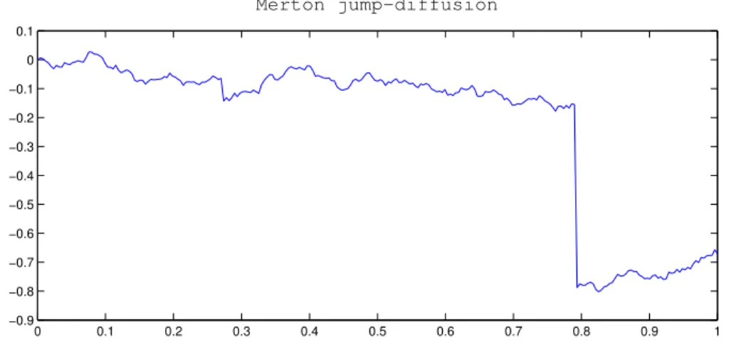
Figure 3.1 represents an example of a simulation of the Merton’s model for illustra-tion purposes.

(28)

0 0.1 0.2 0.3 0.4 0.5 0.6 0.7 0.8 0.9 1 −0.9 −0.8 −0.7 −0.6 −0.5 −0.4 −0.3 −0.2 −0.1 0 0.1 Merton jump−diffusion

Figure 3.1: Simulation of a jump-diffusion path of the Merton’s model

In the horizontal axis, we represent the time in years, ranging from 0 (today) and 1. The values in the vertical axis correspond to the log-returns.

Some of the properties of this model are for example studied in [42] and we are summarizing some of them here.

Let H(ST) be the value of a contingent claim at its maturity (H(ST) = (ST ≠ K)+

in the case of a European call and H(ST) = (K ≠ ST)+ for a European put), H(St) its

intrinsic value at time t œ [0, T] and

HBS(St, ‡, ·, r≠ q) := e≠r·EQ[H(Ste(r≠q≠

‡2

2 )·+ ‡WQ

· )]. (3.2)

The latter corresponds to the pricing formula developed by Black-Scholes-Merton in [10] for a European-style plain vanilla option, where it is supposed that the underlying follows a GBM. Here, St, ‡, r and q represent, respectively, the price of the underlying

asset at time t, the diffusion part associated to the Brownian motion in (2.3), the risk-free rate and the continuous dividend yield inherent to the underlying asset. · := T ≠ t is the time until the maturity.

Let j stand for the number of jumps occurring during the time-period ·, which follows a Poisson distribution. According to [42], the pricing formula for the Merton model is: HM(S) = ÿe ≠⁄·(⁄·)j HBS(S © SejµJ+ j‡2_J 2 ≠⁄(eµJ + ‡2_J 2 _≠1)· , Û ‡2+ j‡ 2 J_{, ·, r}_{≠ q) (3.3)}

(29)

As we can see, it is possible for the jump-diffusion to represent the price of a vanilla call or a put as a weighted average of the standard Black-Scholes-Merton prices.

Define d1 and d2 as:

d1 = ln(St/K) + (r ≠ q + ‡

2_/_{2)(T ≠ t)}

‡ÔT _{≠ t} and d2 = d1≠ ‡ÔT ≠ t.

The prices of a call and put options at time t, under the BSM model, are respectively equal to:

Call_tBSM = e≠q(T ≠t)StN (d1) ≠ Ke≠r(T ≠t)N (d2), (3.4)

P utBSM_t = Ke≠r(T ≠t)N (≠d2) ≠ e≠q(T ≠t)StN (≠d1), (3.5)

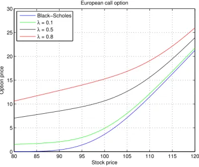
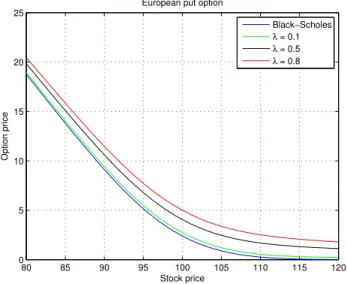
where N represents the cumulative distribution function of the standard normal law. Using the equations above, we plot the Figures 3.2 and 3.3 for illustrative purposes. They represent the price of vanilla options with strike equal to 100, for each spot price, in a range from 80 to 120.

As we can observe, the value of the options under the Merton’s model in comparison with the value under the Black-Scholes model is larger as the rate arrival of jumps increases. It is also possible to show that this also happens when the variance of the jump distribution increases. This was expected, since more jumps with greater variance represent more uncertainty in the expected final payoff and lead to more potential earnings for the option’s owner.

(30)

80 85 90 95 100 105 110 115 120 0 5 10 15 20 25 30

European call option

Stock price Option price Black−Scholes λ = 0.1 λ = 0.5 λ = 0.8

Figure 3.2: Call option prices with

r= 0.05, ‡ = 0.15, q = 0, µJ = ≠0.9, ‡J = 0.45, T = 0.25. 80 85 90 95 100 105 110 115 120 0 5 10 15 20 25 30

European put option

Figure 3.3: Put option prices with

(31)

3.2 Kou’s model

In [33], Kou suggests a jump-diffusion model based in a simple double exponential jump-diffusion. This means the jumps Yi, i œ {0, . . . , Nt} in (2.3) follow a distribution

described as follows:

p(x) := p÷1e≠÷1x11{xØ0}+ (1 ≠ p)÷2e÷2x11{x<0}, ’x œ R, (3.6)

with p, ÷1, ÷2 Ø 0.

For x Ø 0, the expected value of a variable with distribution (3.6) is p ◊ 1

÷1 and for x <0, it is equal to (1 ≠ p) ◊_÷1₂ (when the respective denominators are not null). From

this observation, we interpret p as the probability of occurring an upward jump and (1 ≠ p) the probability of occurring a downward one. Remark that the computation of the first expected value is only possible if ÷1 Ø 1, so that its value is finite. In practical

terms, this means that 1

÷1 <1, i.e, the average jump size cannot exceed 100%, which is

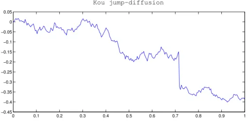
quite an acceptable hypothesis that we shall take in consideration from now on. Figure 3.4 represents a simulation of the path of the log returns of an underlying, following the dynamics described by (2.3), but this time the measure of the jumps is given by (3.6). 0 0.1 0.2 0.3 0.4 0.5 0.6 0.7 0.8 0.9 1 −0.45 −0.4 −0.35 −0.3 −0.25 −0.2 −0.15 −0.1 −0.05 0 0.05 Kou jump−diffusion

(32)

3.2.1 Incremental returns

Quoting [33], "the empirical tests performed in Ramezani and Zeng (2002) suggest that the double exponential jump-diffusion model fits stock data better than the normal jump-diffusion model, and both of them fit the data better than the classical geometric Brownian motion model.". This statement corroborates the fact that the Kou model is suitable for our purpose and one of the reasons it was chosen to price financial derivatives. To better understand why is this true, let us first compute the incremental return of an underlying whose price at time t is St. As stated in the previous chapter,

we are assuming St is the exponential of the Lévy process (2.3). Denoting by an

incremental variation, the incremental return becomes:

St St = St+ t St ≠ 1 = exp IA µ≠1₂‡2 B ( t + t) + ‡Wt+ t+ N_ÿt+ t i=0 Yi J exp IA µ_≠ 1₂‡2 B t+ ‡Wt+ Nt ÿ i=0 Yi J ≠ 1 = exp IA µ_≠1 2‡2 B t+ ‡(Wt+ t≠ Wt) + N_ÿt+ t i=Nt+1 Yi J ≠ 1. (3.7)

If t is sufficiently small (for instance, as when we consider daily observations), the return can be approximated in distribution, ignoring the terms with orders higher than t. Considering the second order approximation in a MacLaurin series of the exponential function (ex _{¥ 1 + x +} 1

2x2), the return of the asset is approximately equal

to: St St ¥ 1 µ_≠ ‡ 2 2 2 t+ ‡(Wt+ t≠ Wt) + N_ÿt+ t i=Nt+1 Yi+ 1₂ A_Ë1 µ_≠‡ 2 2 2 tÈ2 +21µ_≠ ‡ 2 2 2 t_◊Ë‡(Wt+ t≠ Wt) + N_ÿt+ t i=Nt+1 Yi È +Ë‡(Wt+ t≠ Wt) + N_ÿt+ t i=Nt+1 Yi È2B (3.8)

(33)

Now, to simplify the last equation, note the following facts:

• The random variable (Wt+ t≠ Wt) has expected value equal to 0 and variance

t. Concerning the compound Poisson process

N_ÿt+ t

i=Nt+1

Yi, its mean is ⁄ tE(Yi)

and variance ⁄ tE(Y2

i ), as proven in Theorem A.11, found in the Appendix;

• The Brownian motion and the Compound Poisson process are assumed to be independent, so the variance of its sum is equal to sum of the respective variances. Using the last statements, we can imply the following:

• Ë‡(Wt+ t≠Wt)+ N_ÿt+ t

i=Nt

Yi

È

is a random variable with mean ⁄ tE(Yi) and variance

⁄ tE(Y_i2) + ‡2 t. The multiplication of this variable with 21µ_≠ ‡2

2

t makes

this term of order ( t)3 2;

• The expected value of the product of ‡(Wt+ t ≠ Wt) and N_ÿt+ t

i=Nt

Yi is 0 and its

variance is of order ( t)2 _{(it is equal to ‡}2 _t_{◊ ⁄ tE(Y}2

i )); • Ë N_ÿt+ t i=Nt Yi È2

has expected value and variance of at least order o(( t)2_{). The calculus}

involved is not so straightforward as the previous ones, but using the independence of the variables Yi, i œ {Nt+ 1, ..., Nt+ t}, this fact can be proven.

Gathering all this information together, the increment returns become:

St St ¥ µ t + ‡ Ô tZ+ N_ÿt+ t i=Nt+1 Yi (3.9) with Z ≥ N (0, 1).

Appealing to Theorem A.8, found in the Appendix, for ⁄ t small, the probability the Poisson process Nthaving one jump is approximately ⁄ t, having none is 1 ≠ ⁄ t

and more or equal to two is 0. So, we can approximate the summation in the previous SDE as: N_ÿt+ t i=Nt+1 Yi ¥ Y _ ] _ [ Yi, with probability ⁄ t 0, with probability 1 ≠ ⁄ t

(34)

Incorporating this approximation into (3.9), we can write:

St

St ¥ µ t + ‡

Ô

tZ + BY, (3.10)

where B is a Bernoulli random variable with P (B = 1) = ⁄ t and P (B = 0) = 1≠⁄ t and the distribution of Y is given by (3.6).

Notice that without the last part, BY , the last equation corresponds to the GBM, where the incremental return of the underlying follows a normal distribution.

3.2.2 Incremental returns distribution

We are now computing the density distribution of (3.10). In first place, assume

N_ÿt+ t

i=Nt+1

Yi ¥ Yi.

The distribution of the sum of two independent variables is equal to the convolution of the respective density functions (see Theorem A.2) and from that fact, it follows that for any z œ R, the density function of the sum of normal and double-exponential random variables present in (3.10) is equal to:

+Œ_⁄ ≠Œ 1 Ô2fi‡2 _te≠ (z≠x≠µ t)2 2‡2 t ◊ [p÷₁_e≠÷1x11_{xØ0}+ (1 ≠ p)÷₂_e÷2x11_{x<0}]dx = +Œ_⁄ 0 1 Ô2fi‡2 _tp÷1e ≠x2+2x(z≠µ t)≠(z≠µ t)2≠2÷1x‡2 t 2‡2 t _dx + 0 ⁄ ≠Œ 1 Ô2fi‡2 _t(1 ≠ p)÷2e ≠x2+2x(z≠µ t)≠(z≠µ t)2+2÷2x‡2 t 2‡2 t _dx =p÷1e≠ (z≠µ t)2 2‡2 t +Œ_⁄ 0 1 Ô2fi‡2 _te ≠x2+2x(z≠µ t≠÷1‡2 t) 2‡2 t _dx +(1 ≠ p)÷2e≠(z≠µ t)22‡2 t 0 ⁄ ≠Œ 1 Ô2fi‡2 _te ≠x2+2x(z≠µ t+÷2‡2 t) 2‡2 t _dx =p÷1e≠ (z≠µ t)2 2‡2 t _e(z≠µ t≠÷1‡2 t)22‡2 t +Œ ⁄ 0 1 Ô2fi‡2 _te≠ [x≠(z≠µ t≠÷1‡2 t)]2 2‡2 t _dx

(35)

+(1 ≠ p)÷2e≠ (z≠µ t)2 2‡2 t _e(z≠µ t+÷2‡2 t)22‡2 t 0 ⁄ ≠Œ 1 Ô2fi‡2 _te ≠[x≠(z≠µ t+÷2‡2 t)]2_{2‡2 t} _dx =p÷1e≠ (z≠µ t)2 2‡2 t _e(z≠µ t)22‡2 t _e≠2(z≠µ t)÷1‡2 t2‡2 t _e(‡2)2÷21( t)22‡2 t Œ ⁄ 0 1 Ô2fi‡2 _te≠ [x≠(z≠µ t≠÷1‡2 t)]2 2‡2 t _dx +(1 ≠ p)÷2e≠ (z≠µ t)2 2‡2 t _e(z≠µ t)22‡2 t _e2(z≠µ t)÷2‡2 t2‡2 t _e(‡2)2÷22( t)22‡2 t 0 ⁄ ≠Œ 1 Ô2fi‡2 _te≠ [x≠(z≠µ t+÷2‡2 t)]2 2‡2 t _dx =p÷1e≠(z≠µ t)÷1e ‡2÷2_{1 t} 2 Ëz≠ µ t ≠ ÷1‡ 2 _t ‡Ô t È + (1 ≠ p)÷2e(z≠µ t)÷2e ‡2÷2_{2 t} 2 Ë_≠ z≠ µ t + ÷2‡ 2 _t ‡Ô t È ,

where (·) represents the cumulative normal distribution function.

On the other hand, µ t+‡Ô tZ, with Z ≥ N (0, 1), has distribution N (µ t, ‡2 t),

so, its density function is given by: 1 ‡Ô t„ 1_x_{≠ µ t} ‡Ô t 2 ,’x œ R, where „(y) := e≠ 12 y2

Ô2ﬁ ,_{’y œ R is the standard normal density function.}

Thus, for the case

N_ÿt+ t

i=Nt+1

Yi ¥ 0,

the density of (3.10) corresponds to 1

‡Ô t„( x≠µ t

‡Ô t).

Summarizing the previous results, the density function of the approximation for the returns as described in (3.10), denominated by g, can now be written as:

g(x) = 1 ≠ ⁄ t ‡Ô t „ 1_x_{≠ µ t} ‡Ô t 2 + ⁄ t I p÷1e ‡2÷2_{1 t} 2 _e≠(x≠µ t)÷1 A x_{≠ µ t ≠ ‡}2÷1 t ‡Ô t B +(1 ≠ p)÷2e ‡2÷2_{2 t} 2 _e(x≠µ t)÷2 A ≠ x≠ µ t + ‡ 2_÷ 2 t ‡Ô t BJ .

Looking at (3.10) and using expected value’s linearity, we can affirm that the mean of the a random variable with distribution g is µ t + ⁄

A p ÷1 ≠ (1≠p) ÷2 B

t, since the mean

of the normal distribution in (3.10) is µ t and the one of the product of the Binomial random variable and the variable Y is ⁄ t◊

A p ÷1≠ (1≠p) ÷2 B

(36)

variance of the normal distribution, corresponding to ‡2 _t_{, and the one of BY , because}

they are independent. Assuming also that the outcome of the Bernoulli’s variable is in nothing correlated to the outcome of Y, the variance of BY is then:

V ar(BY ) = E[(BY )2] ≠ E2[BY ]

= E[B2_]E[Y2_{] ≠ E}2_[B]E2_{[Y ]}

= E[B2_{](V ar[Y ] + E}2_{[Y ]) + (V ar[B] ≠ E[B}2_])E2_{[Y ]}

= E[B2_{]V ar[Y ] + V ar[B]E}2_{[Y ]}

= E[B]V ar[Y ] + V ar[B]E2_{[Y ]}

= ⁄ t I p(1 ≠ p) A 1 ÷1 + 1 ÷2 B2 + A p ÷21 + (1 ≠ p) ÷22 BJ + t(1 ≠ t) A p ÷1 ≠ (1 ≠ p) ÷2 B2 .

Therefore, the variance of the density function g is given by:

‡2 t+ ⁄ t I p(1 ≠ p) A 1 ÷1 + 1 ÷2 B2 + A p ÷2₁ + (1 ≠ p) ÷2₂ BJ + t(1 ≠ t) A p ÷1 ≠ (1 ≠ p) ÷2 B2 .

3.2.3 Empirical evidence

Figure 3.5 is a plot of the density function g, along with the one corresponding to the normal distribution, both with the same mean and variance.

Figures 3.6, 3.7 and 3.8 represent "zoom-in" plots of the graph of g, respectively evidencing the contrast between the peaks, left and right side tails of the normal law and g. As we can observe, the double-exponential distribution has an asymmetric lep-tokurtic feature for the asset returns as well as fatter tails than the normal distribution with the same mean and variance. The parameters used were the same as in [33].

Kou’s model fits a commonly observed behaviour in the markets: an overreaction and under-reaction to various good or bad news. More precisely, in the absence of outside news, the asset price simply follows a GBM. Good or bad news arrive according to a Poisson process, and the asset price changes in response, depending on the jump size distribution. Because the double exponential distribution has both a high peak

(37)

-0.2 -0.1 0.1 0.2 5 10 15 20 25 30

Kou jump diffusion

Normal distribution with same mean and variance

Figure 3.5: Plot of the density function g and the normal distribution. The parameters used were:

µ= 0.15, ‡ = 0.20, ⁄ = 10, ÷1 = 50, ÷2 = 25, p = 0.3. -0.010 -0.005 0.000 0.005 0.010 22 24 26 28

30 Kou jump diffusion

Figure 3.6: Peak

and heavy tails, it can be used to model both the overreaction (attributed to the heavy tails) and under-reaction (attributed to the high peak) to outside news. Therefore, the

(38)

-0.10 -0.08 -0.06 -0.04 -0.02 0.00 0.2 0.4 0.6 0.8 1.0

Kou jump diffusion

Figure 3.7: Left side tail

0.00 0.02 0.04 0.06 0.08 0.10 0.2 0.4 0.6 0.8 1.0

Kou jump diffusion

Figure 3.8: Right side tail

double exponential jump-diffusion model can be interpreted as an attempt to build a simple model, within the traditional random walk and efficient market framework to incorporate investors’ sentiment. Besides, it also allows for a simple pricing of more complicated and exotic options like path-dependent options as Kou states in [33]. This simplicity makes this model quite popular in the literature, representing an improve-ment in comparison to the BSM model, while it maintains its analytical tractability.

(39)

3.2.4 Option pricing

In order to obtain prices for vanilla options and other financial securities, [33] uses semi-closed formulas which are also used in [42]. However, we are presenting a different approach, based on the framework of Bakshi, Madan, Green and Heston. On page 218 of [3], these authors suggest pricing European vanilla options based on the characteristic function of the random process we consider. This way, the reader has an alternative way for obtaining vanilla option prices which only requires the numerical valuation of integrals. For the Kou’s model case, using (2.2), we can compute the characteristic function of a Lévy process Lt, denoted by „Lt, with a double exponential jump size distribution (3.6) in the following way (for more details, see [44]):

„Lt(u) := E[e

iuLt] = et

Ë

iuµ≠‡2u22 +iu⁄

1 p ÷1≠iu≠ (1≠p) ÷2+iu 2È , (3.11) where µ =1r_{≠ q ≠} ‡2 2 2 .

Using equation (3.11), we can get the characteristic function of the random variable ln(St) which we denote by „ln(St).

The prices of European-style options are then computed as:

Call_tEur = Ste≠q(T ≠t) 1≠ Ke≠r(T ≠t) 2, (3.12) P utEur_t = Ke≠r(T ≠t)(1 ≠ 2) ≠ Ste≠q(T ≠t)(1 ≠ 1), (3.13) where 1 = 1₂+ 1 ﬁ +Œ_⁄ 0 Re1e ≠iuln(K)_„ ln(ST)(u ≠ i) iu„ln(ST)(≠i) 2 du, (3.14) 2 = 1₂+ 1 ﬁ +Œ_⁄ 0 Re1e≠iuln(K)„ln(ST)(u) iu 2 du. (3.15)

The integrals above can be calculated using, for example, a Gauss-Legendre quadra-ture, as done in [21].

The same way we did for Merton, we plot the price of vanilla options, for each spot price, in a range from 80 to 120, with strike equal to 100, using the formulas above (see Figures 3.9 and 3.10 below). The same conclusions are reached as for Merton’s model:

(40)

an increase on the jump intensity leads to an option price increase and for any case, an option price under Kou’s model is more expensive than one priced with BSM model.

80 85 90 95 100 105 110 115 120 0 5 10 15 20 25

European call option

Figure 3.9: Call option prices with

r= 0.05, ‡ = 0.15, T = 0.25, K = 100, q = 0, ⁄ = 0.10, ÷1 = 3.0465, ÷2 = 3.0775, p = 0.3445. 80 85 90 95 100 105 110 115 120 0 5 10 15 20 25

European put option

Figure 3.10: Put option prices with

r= 0.05, ‡ = 0.15, T = 0.25, K = 100,

(41)

4

Incomplete markets

As mentioned in Chapter 2, the assumption that the trading of assets takes place without arbitrage opportunities leads to the existence of a martingale measure Q and the discounted process, ( ˜St)tØ0, is a martingale in the probability space ( , F, Q).

Now, a fundamental question naturally arises: is this measure unique? The answer is: No. In the Lévy models context, there might be several measures that turn the discounted process ( ˜St)tØ0 a martingale. As a consequence of the Second Fundamental

Theorem of Asset Pricing, the market is not complete. This means that it is not possible to construct a self-financing trading portfolio that eliminates the risk of an existing position. In other words, if we acquire a certain financial product, such as a vanilla option, it will not be possible to trade other assets at inception of its acquisition, in such a way we guarantee a perfect hedging. For a better understading of these concepts, we suggest the reading of [9].

We are now giving some insight on why are markets incomplete when assets are driven by Lévy processes, based on [45]. The goal is not at all to present an exhausting prove of this claim, but to provide some results which give an idea of its veracity. Accomplished this goal, we then suggest a measure from among the infinite number of possible choices.

(42)

4.1 The Lévy measure

A convenient tool for analyzing the jumps of a Lévy process is the random measure of jumps of the process. Consider a set A œ B(R \ {0}), where B(R \ {0}) is the Borel

‡-algebra on R \ {0}, such that 0 /œ ¯A. Letting 0 Æ t Æ T, the random measure of the

jumps of the process L is defined by:

’Ê œ , µL(Ê; t, A) := #{0 Æ s Æ t : Ls(Ê) œ A} =

ÿ

sÆt

11A( Ls(Ê)). (4.1)

Hence, the measure µL(Ê; t, A) counts the jumps of the process L of size A up to

time t. It is possible to prove that µLis a Poisson random measure and that its intensity,

defined by

‹(A) = E[µL(1, A)] = E[ÿ

sÆ1

( Ls(Ê))] (4.2)

is a ‡-finite measure on R \ {0}, In (4.2), the first argument Ê was suppressed for simplification purposes.

µL(1, A) measures the number of jumps of size A until t = 1. Thus, the indicator

function in (4.1) equals 1, when the jump is of size A and 0 otherwise. This is how we obtain the last equality in (4.2).

4.2 Incompleteness evidence

Let Q be a probability measure on F, equivalent to P. Its Radon-Nikodym deriva-tive dQ

dP is a non-negative integrable random variable, so, using tower’s law, it is not

difficult to see that the process Zt = EP

Ë

dQ

dP|Ft

È

,’ 0 Æ t Æ T , is a martingale under the probability P and its expected value under this measure equals 1.

To formalize the result in last paragraph, we present the following theorem, found in [45].

Theorem 4.1. Given two equivalent measures P and Q, there exists a unique, positive, P-martingale Z = (Zt)0ÆtÆT such that Zt = EP

Ë

dQ

dP|Ft

È

(43)

Let L = (Lt)0ÆtÆT be a Lévy process with triplet (a, b, ‹) under P, with finite first

moment. Then, L has the canonical decomposition:

Lt= bt + ÔaWt+ ⁄ t 0 ⁄ Rx(µ L ≠ ‹L)(ds, dx).

As referred in [47], in the last stochastic integral of the previous expression, ‹L

represents the compensator of the Poisson random measure µL and it is a product

measure of the Lévy with the Lebesgue measures, letting us therefore write ‹L(ds, dx)

as ‹L(dx)ds.

This author also proves that if P ≥ Q with density process Z, there exists a deter-ministic process — and a measurable non-negative deterdeter-ministic process Y , satisfying

⁄ t 0 ⁄ R|x(Y (s, x) ≠ 1)|‹(dx)ds < Œ and ⁄ t 0 (a— 2 s)ds < Œ, Q-a.s. for 0 Æ t Æ T .

Under the new measure, ˜Wt= Wt≠

⁄ t

0 (Ôa—s)ds is a Brownian motion, ˜‹

L(ds, dx) =

Y(s, x)‹L(ds, dx) is the Q-compensator of µLand L has the following canonical

decom-position under Q: Lt= ˜bt + Ôa ˜Wt+ ⁄ t 0 ⁄ Rx(µ L_{≠ ‹}L)(ds, dx), where ˜bt = bt +⁄ t 0 a—sds+ ⁄ t 0 ⁄ Rx(Y (s, x) ≠ 1)‹ L(ds, dx).

For what we purposed to show, we can suppose, without loss of generality, that — and Y previously mentioned are deterministic and independent of time. Then, in this case:

˜b = b + a— +⁄

Rx(Y ≠ 1)‹

L(dx).

Under the risk neutral measure Q, the asset price has mean rate of return µ = r ≠ q and the discounted process ( ˜St)0ÆtÆT is a martingale under Q. Therefore, according to