Bol. Ciênc. Geod. vol.20 número4

(1)

BCG - Boletim de Ciências Geodésicas - On-Line version, ISSN 1982-2170 http://dx.doi.org/10.1590/S1982-21702014000400054

STUDY ON CYCLE-SLIP DETECTION AND REPAIR

METHODS FOR A SINGLE DUAL-FREQUENCY GLOBAL

POSITIONING SYSTEM (GPS) RECEIVER

Estudo sobre detecção e correção de perdas de ciclos para posicionamento por ponto preciso com receptor GPS de dupla frequência

LA VAN HIEU 1,2 VAGNER G. FERREIRA 1,

XIUFENG HE 1 XU TANG 1,3

1_{School of Earth Sciences and Engineering} Hohai University, Nanjing, China vagnergf@hhu.edu.cn; xfhe@hhu.edu.cn

2_{Centre of Geomatics}

Water Resources University, Hanoi, Vietnam lavanhieu@wru.edu.vn

3_{Faculty of Science and Engineering} University of Nottingham, Ningbo Campus, China

Xu.Tang@nottingham.edu.cn

ABSTRACT

In this work, we assessed the performance of the cycle-slip detection methods: Turbo Edit (TE), Melbourne-Wübbena wide-lane ambiguity (MWWL) and forward and backward moving window averaging (FBMWA). The TE and MWWL methods were combined with ionospheric total electron content rate (TECR), and the FBMWA with second-order time-difference phase ionosphere residual (STPIR) and TECR. Under different scenarios, 10 Global Positioning System (GPS) datasets were used to assess the performance of the methods for cycle-slip detection. The MWWL-TECR delivered the best performance in detecting cycle-slips for 1 s data. The relative comparisons show that the FBMWA-TECR method performed slightly

(2)

Hieu, V. L. et al. 9 8 5 better than its original version, FBMWA-STPIR, detecting 100% and 73%, respectively. For data with a sample rate of 5 s, the FBMWA-TECR performed better than MWWL-TECR. However, the FBMWA is suitable only for post-processing, which refers to applications where the data are processed after the fact. Key words: Cycle-Slip; FBMWA; GPS; MWWL; STPIR; TEC.

RESUMO

Este trabalho apresenta uma investigação do desempenho dos métodos de detecção e correção de perdas de ciclos: Turbo Edit (TE), Melbourne-Wübbena banda larga (MWWL) e forward and backward moving window averaging (FBMWA). Os métodos TE e MWWL foram combinados com a taxa de variação do conteúdo total de elétrons presentes na ionosfera (TECR) e o FBMWA com Second-order Time-difference Phase Ionosphere Residual (STPIR) e TECR. Sob diferentes cenários, dados GPS de 10 estações são utilizados para avaliar o desempenho dos métodos para detecção de perdas de ciclos. O MWWL-TECR apresentou o melhor desempenho na detecção das perdas de ciclo para dados com taxa de observação de 1 s. As comparações relativas mostram que o método FBMWA-TECR apresenta melhores resultados em relação com a versão original FBMWA-STPIR em que a taxa de detecção foi de 100% e 73%, respectivamente. Para dados com taxa de amostragem de 5 s, o FBMWA-TECR apresentou melhor desempenho do que MWWL-TECR. No entanto, o FBMWA é adequado apenas para pós-processamento, que se refere a aplicações em que os dados GPS são processados após o rastreio.

Palavras chave: Perda de Ciclo; FBMWA; GPS; MWWL; STPIR; TEC.

1. INTRODUCTION

Cycle-slip detection and correction is an important aspect when using global navigation satellite systems (GNSSs), e.g., the Global Positioning System (GPS), in any application that needs carrier phase data (BANVILLE and LANGLEY, 2013). Nowadays, single dual-frequency receivers (i.e., only one GPS receiver) are used in many applications, such as the precise point positioning (PPP) technique for geohazard monitoring, crustal-deformation monitoring, ocean tide measuring and, atmosphere water vapour sensing among others, in GNSS-remote sensing (see, e.g., KHANDU et al., 2011; AWANGE, 2008; GENG et al., 2011; JIN et al., 2011). In these examples, the GPS signal could be temporarily lost due to the obstruction of the signal between the GPS satellite and the receiver antenna. Under such conditions, the GPS data are subject to a cycle-slip. A cycle-slip causes a discontinuity in the carrier phase, observable by an integer number of cycles (LEICK, 2004). Thus, when processing GPS carrier phase data, the detection and reparation of cycle-slips is mandatory (DAI, 2012).

(3)

Study on cycle-slip detection and repair methods for a... 9 8 6

1999; BISNATH, 2000; COLOMBO et al., 1999; KIM and LANGLEY, 2001; LEE et al., 2003). However, they are not suitable for PPP or other applications that require single GPS receiver data. Moreover, some methods are based on the integration of the GPS and inertial navigation system (INS) data (see, e.g., COLOMBO et al., 1999; ALTMAYER, 2000; LEE et al., 2003; DU and GAO, 2012). These methods, therefore, significantly constrain their feasibility in many applications due to the cost of the INS system as well as the complexity of adding an INS system to GPS.

General cycle-slip detection methods, such as code comparison, phase-phase ionospheric residual, Doppler integration, and differential phase-phase of time, have their own limitations. The phase-code comparison method, for instance, is not effective in repairing small cycle-slips due to the low accuracy of the code measurements. The phase-phase ionospheric residual method, which is essentially the geometry-free linear combination, has a shortcoming of being insensitive to special cycle-slip pairs and unable to check on which frequency the cycle-slip happens (XU, 2007). The differential phase of time method requires polynomial fittings to interpolate or extrapolate the data at the check epoch (XU, 2007). However, tests performed by Liu (2010) indicate that the polynomial cannot guarantee success all the time, particularly, when the size of the cycle-slip is small. Further, the Doppler integration method, like phase-code comparison, fails to detect small cycle-slips (LIU, 2010).

The research on cycle-slip detection using single GPS receiver data is less than the research based on double-differencing GPS data. The work of Blewitt (1990) was the first effort in cycle-slip detection and repair for single GPS data. It introduced an automatic editing algorithm (Turbo Edit – TE) which proposed using simultaneously the wide-lane combination and ionospheric combination to detect the cycle-slip. The wide-lane combination used in Blewitt (1990) is essentially the same as the Melbourne-Wübbena linear combination. This combination is very effective for cycle-slip detection because of its low level of noise and its insensitivity to ionospheric changes. Incorrect cycle-slip determination may be caused when there are rapid ionospheric variations (BLEWITT, 1990). De Lacy et al. (2008) proposed a Bayesian approach to detect cycle-slip for single GPS receivers. The basic assumption of this method is that the original signal is smooth and discontinuities (i.e., the cycle-slip) can be reasonably modelled by a multiple polynomial regression (DE LACY et al., 2008). However, Liu (2010) pointed out that this assumption may be valid in most cases; however, it is not valid when the GPS data are observed under high level ionospheric activities. Additionally, Zhang et al. (2012) proposed a new approach for single frequent cycle-slip detection based on an autoregressive model by exploiting modern Bayesian statistical theory.

(4)

Hieu, V. L. et al. 9 8 7 undergoes rapid variations (e.g., LIU, 2010). Wu et al. (2010) also proposed a method based on the use of multi-frequency GPS carrier phase observations. Liu (2010) introduced a new automated cycle-slip detection and repair method for a single dual-frequency GPS receiver. This method jointly uses the ionospheric total electron content (TEC) rates (TECR) and Melbourne-Wübbena wide-lane linear combination to uniquely determine the cycle-slip on both L1and L2 frequencies (LIU, 2010). However, this approach is effective for high sampling rate data such as 1 s. As a matter of fact, many geodetic applications require data with 1s sampling data, for example, the Gravity Recovery and Climate Experiment (GRACE) satellite mission.

However, in applications with low sampling data (e.g., 30 s), the above mentioned method does not deliver satisfactory results. To overcome this shortcoming, Cai et al. (2012) proposed a new cycle-slip detection method that is effective for low sampling rate data such as 30 s. This is an important aspect since many receivers have a limitation on the storage capacity and, for example, many continuously operating reference stations (CORS) use the 30-s sample rate. In this approach, a forward and backward moving window averaging (FBMWA) algorithm and a second-order time-difference phase ionospheric residual (STPIR) algorithm are integrated to jointly detect and repair cycle-slips. The FBMWA algorithm is proposed to detect cycle-slips from the wide-lane ambiguity of the Melbourne-Wübbena linear combination observable. The FBMWA algorithm has the advantage of reducing the noise level of wide-lane ambiguities, even if the GPS data are observed under rapid ionospheric variations.

Nevertheless, few comparisons of the algorithms used to detect and repair cycle-slips for non-differentiated GPS observations have been made so far. Further, we combined the TE and Melbourne-Wübbena wide-lane ambiguity (MWWL) with TECR (i.e., TE-TECR and MWWL-TECR) and FBMWA with TECR and with STPIR (i.e., FBMWA-TECR and FBMWA-STPIR). Additionally, a slightly modified version of the FBMWA by adding the TECR is also proposed.

2. DATA SET AND METHODS

2.1 Data Description

(5)

Study on cycle-slip detection and rep 9 8 8

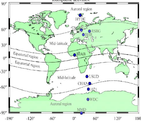
example, BJAB is under a region where the scintillation effects ar approximately ±10° of magnetic latitude). It is well known that s sufficiently intense, cause GPS receivers to stop tracking the sign satellites in the so-called “loss of loc” process (e.g., KINTNER et particular choice of these points is due to the fact that they are regions subject to ionospheric effects, such as the polar cap, auroral, a (Figure 1). In the auroral region, scintillation effects occur mainly w geomagnetic storms, while in the equatorial region their occurr common due to the intensity of the TEC and equatorial anomalies.

Figure 1 – Distribution of GPS stations used for assessing the perfor cycle-slip detection and repair methods. Additionally, regions of the w

ionospheric activities.

Table 1 summarizes the information on these 10 GPS data se sets give 24-hour observations (two data sets with 5-s intervals, five 30-s intervals). Three other data sets give 1-hour observations with 1s

repair methods for a... are strongest (at t scintillations, if ignals from GPS et al., 2007). The re located within l, and sub-auroral y when there are urrence is more

formance of the e world with high

(6)

Hieu, V. L. et al.

Table 1 – Summary of GPS data used in this st Date Station Sample Receiv 2012/05/29 1021

1 s

ASHTECH

2011/03/11 USUD ASHTECH

2014/01/01 MMD NOV WA

2014/01/01 RSBG _{5 s} LEICA GRX12

2012/11/30 TN02 DL-V3-L

2011/03/11 BJAB

30 s

TRIMBLE 2014/04/10 CHAN _HYDE _{LEICA GRX12}ASHTECH

2001/03/31 _WDCBHR ZY12_ZY12

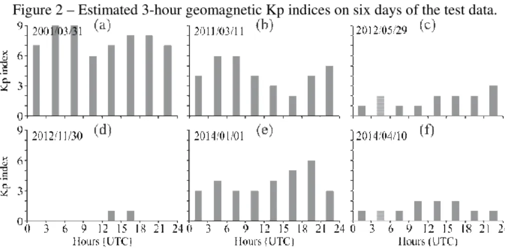
Figure 2 shows the geomagnetic Kp indices on six days values of the Kp indices (an integer in the range 0–9) chan 2012/11/30) to geomagnetic storm (Kp 5; e.g., 2001/03/31).

Figure 2 – Estimated 3-hour geomagnetic Kp indices on six d

In Figure 2 (a) and (b), we can identify two especial d 2011/03/11, respectively. On the first day (2001/03/31, Figure Kp index reached 9 as a strong interplanetary shock wave s produced one of the largest geomagnetic storms (BAKER, 20 was very active on 31st_{March 2001, and its daily Kp indices (s} minimum values in Figure 2 (a)) are the highest in the past 2 and the 6th_{highest in the past 80 years (1932–2011). The io} observed to increase to 100 TECU during the 31st March 200 al., 2002). The second day with a high Kp index is 2011/03/11

9 8 9

study. eiver

H UZ-12 H UZ-12 AASGII 1200+GNSS L1/L2S E NETR5

H UZ-12 1200GGPRO

12 12

ys of the test data. The hange from calm (e.g.,

x days of the test data.

(7)

four years without any X-flares, the Sun produced two powerful blasts in less than one month, i.e., 15th _{February and 9}th _{March. On 11}th _{March, the Earth’s magnetic} field was still reverberating from a coronal mass ejection (CME) strike on 10th March.

2.2 Cycle-slip Detection

2.2.1 TE Algorithm and TECR

The TE algorithm provided by Blewitt (1990) is an algorithm for cycle-slip detection and repair as well as for outlier removal using non-differentiated dual-frequency GPS data. The TE algorithm is based on Melbourne-Wübbena (MW) and the geometry-free combinations. The well-known MW wide-lane linear combination at a given epoch,

1 1 1 2 2 2 1 1 2 2

MW WL WL

1 2 1 2

f f f P f P

L N

f f f f

λ

Φ −

λ

Φ −

_λ

= − =

− + , (1)

can be estimated by considering that at the epoch (k−1) there was no cycle-slip or that it has been repaired already. However, at the epoch k there are cycle-slips on both theL₁ and L₂ carrier phase measurements Φ₁( )k and Φ₂( )k . The variables in Equation (1) are, f1 and f2 the carrier frequencies; λ1 and λ2 the wavelengths of theL₁ and L₂ signals; P₁ and P₂ the pseudo-ranges on the L₁ and L₂ frequencies.

The wide-lane ambiguity, NWL, is

MW 1 1 2 2

WL 1 2

WL WL( 1 2)

L f P f P

N

f f

λ

+

= = Φ − Φ −

+ . (2)

As long as the phase observations are free of cycle-slips, the wide-lane ambiguity remains quite stable over time (CAI et al., 2012).

In utilizing the MW combination to detect cycle-slips, a recursive averaging filter can be used as follows (BLEWITT, 1990):

[

WL

]

WL WL WL WL

1

E N ( )k N ( )k N (k 1) N ( )k N (k 1) k

 

= = − +  − −  (3)

with the standard deviation of NWL( )k as:

(

)

WL WL WL

2

2 2 2

( ) ( 1) WL WL ( 1) 1

( ) ( 1)

N k N k N k N k N k

k

σ

₌

σ

₋ ₊  ₋ ₋ ₋

σ

₋ 

 

(8)

Hieu, V. L. et al. 9 9 1 whereNWL( )k is the mean value of NW L( )k , k and (k-1) are the present and previous epochs, respectively. The calculation of the mean is exact and the standard deviation has the diminishing error term ₍₁ 2₎

k

O ; however, an initial value of 0.5 cycles is necessary for the standard deviation at the first epoch (LIU, 2010).

When a cycle-slip occurs, the conditions are satisfied as follows:

WL( ) ( 1) 4 ( )

N k −N k− ≥

σ

k

(5) and

WL( 1) ( ) 1

N k+ −N k ≤ . (6)

Additionally, the method can be complemented with the TEC and its rate (TECR, mathematically defined by TEC′) as proposed by Liu (2010). If the TEC estimated at epoch (k) is differentiated with that of epoch (k−1), the TECR can be computed using the backward difference operator as:

TEC( ) TEC( 1)

TEC ( )k k k

t

− −

′ =

∆ , (7)

where∆t is the time interval between epochs (k) and (k−1).

From a practical point of view, the TEC ( )′ k is estimated based on the measurements of the previous epochs in relation to epoch k as:

TEC ( ) TEC (

′

k

=

′

k

− −

1) TEC (

′′

k

− ⋅∆

1)

t

₍₈₎

where the TEC acceleration (TEC′′; i.e., the second derivative of TEC) at epoch (k – 1)is estimated as:

TEC ( 1) TEC ( 2)

TEC (k 1) k k

t

′ − − ′ −

′′ − =

∆ ₍₉₎

(9)

[

]

[

]

[

1 1 2 2

]

6

1 1 2 2 2

1

1 1 2

1 1

2 2

40.3 10 ( 1) TEC ( )

( ) ( )

[ ( ) ( 1)]

[ ( ) ( 1)

( ) ( )

( ) ( ) ]

N k N k

t k

N k N k

f

k k

k

N k N k k

γ λ λ λ λ λ λ λ λ ∆ − ∆ = ∆ − ′ × − ∆ ⋅ ∆ − ∆ = −

Φ − Φ − +

Φ − Φ

= −

∆

⋯

⋯ . (10)

where 2 2

1 2

f f

γ

= is the ratio of the squared frequencies of the GPS L1 and L2 signals.

2.2.2 Melbourne-Wübbena Wide-Lane and TECR Combination

The Melbourne-Wübbena wide-lane (MWWL) algorithm for cycle-slip detection was first proposed by Blewitt (1990) as mentioned in sub-section 2.2.1. However, Liu (2010) proposed a joint combination of MWWL and the TECR, i.e., MWWL-TECR for detecting and repairing the cycle-slips. Therefore, Liu (2010) proposed an improved variance estimation as:

(

)

(

)

WL

2 2

2

( ) E WL( ) WL( )

N k N k N k

σ

₌  ₋

  ₍₁₁₎

where the variance in TE is provided by (4) and in MWWL-TECR by (11). The

(

)

2

WL

E_ N ( )k _in Equation (10) is the mean squared value of NWL( )k , and it can be calculated recursively as (LIU, 2010):

(

)

2

(

)

2

{

(

)

2

(

)

2

}

WL WL WL WL

1

E N ( )k E N (k 1) N ( )k E N (k 1)

k

 ₌  ₋ ₊ ₋  ₋ 

     

(12) The mean and variance, at epoch (k), of the wide-lane ambiguity can be estimated based on all the data prior to epoch (k). Moreover, Equations (11) and (12) do not require initial value to be given at the first epoch as in (4).

If the cycle-slip term,

[

∆N k1( )− ∆N k2( )

]

=NWL(k− −1) NWL( )k , (13)

(10)

Hieu, V. L. et al. 9 9 3 2.2.3 FBMWA Algorithm

The FBMWA filter algorithm was proposed by Cai et al. (2012). In FBMWA, the wide-lane ambiguity is smoothed in both forward and backward directions with a specified size of smoothing window in each direction. This differs from the regular TE algorithm where only backward smoothing is performed and the window size continuously grows with the number of epochs. Note that the use of a forward smoothing algorithm implies that the FBMWA method is only suitable for post-processing GPS data while TE and MWWL can be used for real time applications.

The FBMWA algorithm is described as follow (CAI et al., 2012):

B WL WL 1 1 F WL WL 1

( 1) ( )

1 ( ) ( ) k m i k k n i k

N k N i

m

N k N i

n − = − + − = − = =

∑

, (14)

where B WL( 1)

N k− is the backward smoothing wide-lane ambiguity over m epochs prior to epoch k and NWLF ( )k is the forward smoothing wide-lane ambiguity over

n epochs at and after epoch k . The difference between F

WL( )

N k _andNWLB (k−1), which provides:

F B

WL( ) WL( ) WL( 1)

N k N k N k

∆ = − − , (15)

can be used to detect the cycle-slip in the wide-lane observation (CAI et al., 2012). The standard deviation,

σ

_FBMWA

( )

k

, of the FBMWA algorithm can be estimated as:

2 2 2

FBMWA( )k F( )k B(k 1)

σ

=

σ

+

σ

− , (16)

Where the terms 2 F

σ

and 2 B

σ

can be computed by using Equation (4). When a cycle-slip occurs, the conditions are satisfied as follows:

WL( 1) WL( ) 4 FBMWA( )

N k− −N k ≥

σ

k . (17)

Based on the FBMWA algorithm (14) and the method to calculate the value of the standard deviation in the MWWL equation, a modified FBMWA is proposed. The variance 2

F

σ

and 2 B

(11)

(

)

( )

(

)

( )

2 2 2 F F WL 2 2 2 B B WL ( ) ( 1)

E N k N

σ

 

= _ _−

 

= _ − _− . (18)

2.2.4 The Second-Order Time-difference Phase Ionospheric Residual Algorithm In the FBMWA algorithm, the cycle-slip in the wide-lane observation can be determined from (15). However, Cai et al. (2012) pointed out that how large the cycle-slips are and in which frequency they occur are still unknown. Hence, Cai et al. (2012) recommend the use of an additional equation for cycle-slip detection, for example, by using the STPIR method.

The phase ionospheric residual (PIR) method is essentially a scaled geometry-free combination, which is defined as follows (CAI et al., 2012):

1 1 2 2 1 1 2 2

(

1)

GF

λ

N

λ

N

γ

I

Φ = Φ − Φ =

−

+ −

₍₁₉₎

where

I

is the ionospheric range delay in metres on

L

₁. The PIR combination is defined as follows (CAI et al., 2012):

GF 2

PIR 1 2 res

1 1

N λ N I

λ λ

Φ

Φ = = − +

(20)

where

I

res is the residual ionospheric error in cycles calculated as

(

γ

−

1)

I

λ

1. The cycle-slip at epoch (k), if any, can be estimated by differentiating the PIR combinations at epochs k and k−1 as (CAI et al., 2012):

[

] [

]

2

1 2 PIR PIR res res 1

( ) ( 1) ( ) ( 1)

N λ N k k I k I k

λ

 

∆ − ∆ = Φ − Φ − − − −

 

  . (21)

Equation (21) is called the first-order time difference of the PIR combination. To minimize the impact of ionospheric disturbances, the STPIR algorithm is proposed. The STPIR algorithm is defined as (CAI et al., 2012):

[

]

[

]

[

]

2

1 2 PIR PIR PIR 1

res e r

1 2 rs es

( ) 2 ( 1) ( 2)

N N k k k

I k I k

ddN I

N d k

λ λ

 

− = Φ − Φ − + Φ − −

 

 

− − +

− = −

⋯

(12)

Hieu, V. L. et al. 9 9 5 In the STPIR (22), the ionospheric residual is significantly smaller than in the first-order time-difference PIR (21).

To detect the cycle-slip at epoch (k), however, the mean variance of ΦPIR data prior to epoch (k) are recursively calculated using a similar approach as shown in Equations (3), (11) and (5).

2.3 Combination of Algorithms to Detect Cycle-slips

If we use any cycle-slip detection algorithm alone, in some cases it cannot detect cycle-slips. For example, the MWWL cannot detect cycle-slip pairs when

1 2

N

∆ = ∆

, e.g., (1,1) and (2,2), where the first number within the brackets is the number of cycles on the L1and the second number the cycles on the L2carrier phase measurements. The STPIR algorithm cannot detect cycle-slip pairs where

1 2

/

1 2

N

λ λ

N

∆ =

∆

, e.g., (77,60) and (18,14). Further, when cycle-slips are detected it is impossible to tell whether

L

1or

L

2or both frequencies have the cycle-slips. That is why the combination of two algorithms is needed.

The cycle-slip pairs

(

∆

N

₁

,

∆

N

₂

)

can be uniquely determined by combining:

1 2

N

a

∆ −∆ =

₍₂₃₎

and

1

N

1 2

N

2

b

λ

∆ − ∆ =

λ

₍₂₄₎

or

2

1 2

1

N λ N b

λ

∆ − ∆ =

(25) That is, combing Equations (23) and (24) or combing (23) and (25).

3. RESULTS AND DISCUSSIONS

3.1 Detection Cycle-slip for 1-second Data

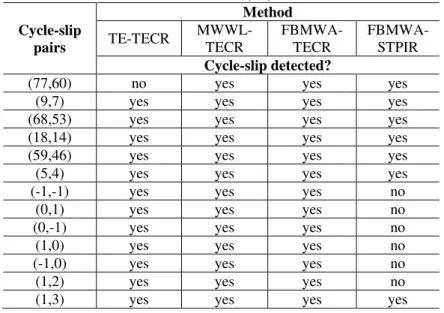
Table 2 shows the results of the comparisons by using the methods TE-TECR, MWWL-TECR, FBMWA-TECR, and FBMWA-STPIR for satellite pseudo range noise (PRN) 9 tracked at station 1021 with a data rate of 1 s.

(13)

ionospheric activity from quiet to active. From columns 2 and 4, it can be seen that TE-TECR cannot detect almost all cycle-slip pairs, while FBMWA-TECR cannot detect small cycle-slip pairs, i.e., (-1,-1), (0,1), (0,-1), (1,0), and (-1,0). It is also noted that the TE-TECR fails to detect the cycle-slip pair (77,60). Thus, it is clear that FBMWA-TEC performs better than TE-TECR under this particular condition.

Table 2 –Results of cycle-slip detection for PRN 9 observed at station 1021 (1 s).

Cycle-slip pairs

Method

TE-TECR MWWL-_TECR FBMWA-_TECR FBMWA-_STPIR Cycle-slip detected?

(77,60) no yes yes yes

(9,7) no no yes yes

(18,14) yes no yes yes

(5,4) yes yes yes yes

(-1,-1) yes yes yes no

(0,1) no yes no no

(0,-1) no no no no

(1,0) no no no no

(-1,0) no no no no

(1,2) no yes yes no

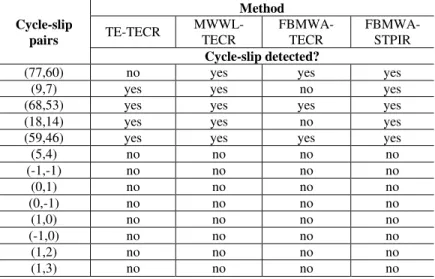
Table 3 shows exactly the same results as Table 2 for station 1021, but for the satellites PRN 12, 18, 22, 25, and 31 while Table 2 shows only PRN 9. For these particular satellites, one can see that only the combination of MWWL-TECR and FBMWA-TECR detected 100% of the cycle-slip pairs. The TE-TECR presents a better performance in comparison with Table 2, however, it could not detect the pair (77,60). Furthermore, as shown in Tables 2 and 3, the TECR detects all small cycle-slip pairs while STPIR failed to detect them. Thus, in this particular experiment, TECR was better than STPIR in detecting small cycle-slip pairs.

(14)

Hieu, V. L. et al.

Table 3 – Results of cycle-slip detection for PRNs 12, 18, 22, 2 station 1021 (1 s).

Method TE-TECR MWWL-_TECR FBMWA-_TECR

Cycle-slip detected?

(77,60) no yes yes

(9,7) yes yes yes

(68,53) yes yes yes

(18,14) yes yes yes

(59,46) yes yes yes

(5,4) yes yes yes

(-1,-1) yes yes yes

(0,1) yes yes yes

(0,-1) yes yes yes

(1,0) yes yes yes

(-1,0) yes yes yes

(1,2) yes yes yes

(1,3) yes yes yes

Figure 3 – Elevation angle of the satellites observed at station 2012/05/29.

Table 4 shows the comparisons for station USUD for all P It can be seen that all combinations failed to detect the small reason is the effect of the strong geomagnetic storm on 2011/ thus the cycle-slip detection ability of the TECR method is redu the worse for STPIR and better for MWWL-TECR, and FBMW the pair (1,2) while FBMWA-TECR failed.

9 9 7

, 25 and 31 observed at

FBMWA-STPIR

yes yes yes yes yes yes no no no no no no yes

n 1021 over 1 hour on

(15)

Table 4 – Results of cycle-slip detection for all PRNs observed at station USUD (1 s).

Method

TE-TECR MWWL-_TECR FBMWA-_TECR FBMWA-_STPIR

(-1,-1) no yes no no

(0,1) no no no no

(0,-1) no no no no

(1,0) no no no no

(-1,0) no no no no

(1,2) yes yes no yes

Table 5 shows the comparison results of cycle-slip detection for all PRNs of station MMD (1 s). Although the Kp value is medium (see Figure 2 (e)), station MMD (geomagnetic latitude 80.26°) is located near to the centre of the polar cap region. Hence, not all small cycle-slip pairs could be detected.

Table 5 – Results of cycle-slip detection for all PRNs observed at station MMD (1 s).

Method

TE-TECR MWWL-_TECR FBMWA-_TECR FBMWA-_STPIR

(5,4) no no no no

(-1,-1) no no no no

(0,1) no no no no

(0,-1) no no no no

(1,0) no no no no

(-1,0) no no no no

(1,2) no no no no

(16)

Hieu, V. L. et al. 9 9 9 3.2 Detection Cycle-slip for 5-second Data

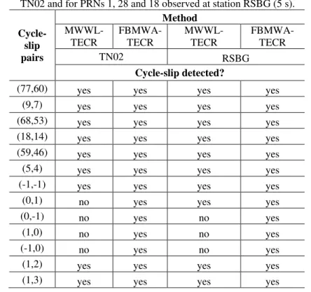
In Table 6 the comparisons of the cycle-slip detection methods are presented for stations TN02 and RSBG. Both stations are located in the sub-aurora region and the data sets were collected on 2012/11/30 and 2014/01/01 for RSBG and TN02, respectively. The value of the Kp index at the time of each data set was medium (mean value of 4.0), the stations stayed in the sub-aurora region, and had no solar flare when the data sets were collected. Thus, although the rate of the data (5 s) is not small, all cycle-slip can be easily detected in such situations. The combination of FBMWA-TECR detected all cycle-slip pairs for both stations while the combination MWWL-TECR could not detect the small cycle-slip. Thus, it can be seen that the combination FBMWA-TECR is better than combination MWWL-TECR for these two stations under their environmental conditions. Additionally, the calculated cycle-slip values are exactly the same for both methods and there are no cycle-slip noises.

Table 6 – Results of cycle-slip detection for PRNs 17, 21 and 32 observed at station TN02 and for PRNs 1, 28 and 18 observed at station RSBG (5 s).

Cycle- slip pairs

Method

MWWL-TECR FBMWA-TECR MWWL-TECR FBMWA-TECR

TN02 RSBG

(77,60) _yes _yes _yes _yes

(-1,-1) yes yes yes yes

(0,1) _no _yes _yes _yes

(0,-1) no yes no yes

(1,0) no yes no yes

(-1,0) no yes no yes

(17)

Study on cycle-slip detection and repair methods for a... 1 0 0 0

3.2 Detection Cycle-slip for 30-second Data

Table 7 shows that the same size of cycle-slip has more prominent impact on the TECR when the data interval is smaller. When one cycle-slip occurs on data

with an interval of 30 s for example, it causes a TECR change of only -0.017TECU/s. This magnitude is very close to the nominal TECR value in the quiet

ionosphere period and is even smaller than the value under active ionosphere conditions, which implies that detecting small cycles with a low data rate is a challenge (LIU, 2010).

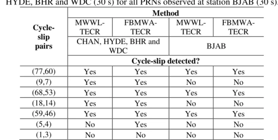
To demonstrate the results in Table 7, stations CHAN and BHR located in the mid-latitude region, stations HYDE and WDC located at the polar cap and station BJAB located at the equator were analysed with 30-s data. The Kp indices for these five stations range from medium to very high (Figure 2). The data sets of stations BHR and WDC were collected during a strong geomagnetic storm and station BJAB during a strong solar flare. The results of cycle-slip detection for stations CHAN, HYDE, BHR and WDC are presented in Table 8. It can be seen that the results for all data sets are the same and the differences in the Kp index values only affect the small cycle-slip detection ability.

Table 7 – The effect of cycle-slip on TEC and TECR.

1( ) 2( )

N k N k

∆ = ∆ Effect on TEC _(TECU) Effect on TECR (TECU/s) Data sample rate 1.0 s 5.0 s 30.0 s

1 -0.506 -0.506 -0.101 -0.017

2 -1.017 -1.017 -0.203 -0.034

3 -1.518 -1.530 -0.306 -0.051

4 -2.024 -2.043 -0.409 -0.068

5 -2.530 -2.556 -0.511 -0.085

Table 8 – Statistical results of cycle-slip detection for all PRNs for stations: CHAN, HYDE, BHR and WDC (30 s) for all PRNs observed at station BJAB (30 s).

Cycle- slip pairs

Method

MWWL-TECR FBMWA-TECR MWWL-TECR FBMWA-TECR CHAN, HYDE, BHR and

WDC BJAB

(77,60) Yes Yes Yes Yes

(9,7) Yes Yes No No

(18,14) Yes Yes No No

(5,4) No Yes No No

(18)

Hieu, V. L. et al. 1 0 0 1

In Table 5, for station MMD, located in the polar cap region and observed with a high data rate (1 s), the cycle-slip pair (5,4) was not detected. In Table 8, however, stations HYDE and WDC, far from the centre of the polar cap region (in terms of geomagnetic coordinates), were observed with the low data rate (30 s) and cycle-slip pair (5,4) was detected. Thus, the station’s location plays a crucial role in cycle-slip detection rather than the level of the data rate (the values of the interval). However, the results of the FBMWA-TECR combination show many small cycle-slip noises which are not present in the results of the MWWL-TECR. Thus, the MWWL-TECR combination is still the best method of cycle-slip detection. Despite the properties of the data sets being different, Tables 6 and 8 show that not all small cycle-slips were detected.

4. SUMMARY AND CONCLUSIONS

In this work we assessed the performance of the cycle-slip detection methods TE; MWWL; and FBMA and the combination of the first two methods (i.e., TE and MWWL) with ionospheric TECR, and the FBMWA with STPIR and TECR. Additionally, we modified the estimation of the variance in the original FBMWA method. Overall, the results showed that the algorithm worked well even in the case of intensive cycle-slips and it seems that the intensity of the cycle-slips did not affect the performance of the methods. However, accuracy was slip-size dependent since different cycle-slip sizes, i.e., (77,60), (9,7), (68,53), (18,14), (59,46), (5,4), (-1,-1), (1,1), (0,1), (0,-1), (1,0), (-1,0), (1,2), (1,3), and (1,5) were tested. The MWWL-TECR delivered the best performance in detecting cycle-slips for 1s data. However, the method failed in detecting small cycle-slip pairs for a station located in the mid-latitude region under a strong geomagnetic storm occurring on11th _March 2011. Furthermore, it is worth mentioning that the type of event that occurred on 11th_{March 2011 is rare. Overall, the method showed a very high detection ratio,} with higher accuracy in the case of large cycle-slips, achieving approximately a 67% detection ratio. The almost 43% of undetected cycles slips is due to the combinations of small cycle-slips with station MMD located in a very active region in terms of ionosphere and USUD under a geomagnetic storm.

(19)

while STPIR is effective when

λ

1

∆ − ∆ ≠

N

1

λ

2

N

2

0

. In all conditions, all cycle-slip pairs were detected, except pair (1,1) when the value of the second time difference noise was over 0.287 cycles. The errors in the calculated cycle-slips are region dependence, data rate sample, sensitivity to solar flares and geomagnetic storm activity. The error from the low-rate data is about 0.64 cycles while for the high ionospheric activity it is about 1.42 cycles. The error from the polar cap (or equator) region is over one cycle. In many cases, the neighbouring cycle-slips affected the cycle-slips; hence, in such a situation it is recommended to run the algorithm again.

ACKNOWLEDGEMENTS

Vagner G. Ferreira acknowledges the National Natural Science Foundation of China (Grant No. 51208311). Xiufeng He acknowledges the National Natural Science Foundation of China (Grant No. 41274017).We acknowledge the Associate Editor and the two reviewers for their remarks which helped to improve the manuscript.

REFERENCES

ALTMAYER, C. Enhancing the integrity of integrated GPS/INS systems by cycle slip detection and correction. In: Proceedings of the IEEE Intelligent Vehicles Symposium 2000 (Cat. No.00TH8511). p.174–179, 2000. Dearborn, MI: IEEE. AWANGE, J. Environmental Monitoring Using GNSS: Global Navigation Satellite

Systems. Springer, 2008. 382 p.

BAKER, D. N. A telescopic and microscopic view of a magnetospheric substorm on 31 March 2001. Geophysical Research Letters, v. 29, n. 18, p. 1862, 2002. BANVILLE, S.; LANGLEY, R. B. Mitigating the impact of ionospheric cycle slips

in GNSS observations. Journal of Geodesy, v. 87, n. 2, p. 179–193, 2013. BASTOS, L.; LANDAU, H. Fixing cycle slips in dual-frequency kinematic

GPS-applications using Kalman filtering. Manuscripta Geodetica, v. 13, n. 4, p. 249–256, 1998.

BISNATH, S. B.Efficient, automated cycle-slip correction of dual-frequency kinematic GPS data. In: Proceedings of the 13th International Technical Meeting of the Satellite Division of The Institute of Navigation (ION GPS 2000), p. 145–154, 2000. Salt Lake City, UT.

BLEWITT, G. An Automatic Editing Algorithm for GPS data. Geophysical Research Letters, v. 17, n. 3, p. 199–202, 1990.

CAI, C.; LIU, Z.; XIA, P.; DAI, W. Cycle slip detection and repair for undifferenced GPS observations under high ionospheric activity. GPS Solutions, v. 17, n. 2, p. 247–260, 2012.

(20)

Hieu, V. L. et al. 1 0 0 3 Institute of Navigation (ION GPS 1999). p.1915–1922, 1999. Nashville, TN: ION.

DAI, Z. MATLAB software for GPS cycle-slip processing. GPS Solutions, v. 16, n. 2, p. 267–272, 2012.

DAI, Z.; KNEDLIK, S.; LOFFELD, O. Instantaneous triple-frequency GPS cycle-slip detection and repair. International Journal of Navigation and Observation, v. 2009, p. 1–15, 2009.

DU, S.; GAO, Y. Inertial aided cycle slip detection and identification for integrated PPP GPS and INS. Sensors, v. 12, n. 11, p. 14344–14362, 2012.

FOSTER, J. C.; ERICKSON, P. J.; GOLDSTEIN, J.; RICH, F. J. Ionospheric signatures of plasmaspheric tails. Geophysical Research Letters, v. 29, n. 13, p. 1–4, 2002.

GENG, J.; TEFERLE, F. N.; MENG, X.; DODSON, A. H. Towards PPP-RTK Ambiguity resolution in real-time precise point positioning. Advances in Space Research, v. 47, n. 10, p. 1664–1673, 2011.

JIN, S.; FENG, G. P.; GLEASON, S. Remote sensing using GNSS signals: Current status and future directions. Advances in Space Research, v. 47, n. 10, p. 1645–1653, 2011.

KHANDU; AWANGE, J. L.; WICKERT, J.; SCHMIDT, T.; SHARIF, M. A.; HECK, B.; FLEMING, K. GNSS remote sensing of the Australian tropopause. Climate Change, v. 115, n. 3–4, p. 597–618, 2011.

KIM, D.; LANGLEY, R. Instantaneous real-time cycle-slip correction of dual frequency GPS data. In: Proceedings of the International Symposium on Kinematic Systems in Geodesy, Geomatics and Navigation. p.255–264, 2001. KINTNER, P. M.; LEDVINA, B. M.; DE PAULA, E. R. GPS and ionospheric

scintillations. Space Weather, v. 5, n. 9, p. S09003, 2007.

DE LACY, M. C.; REGUZZONI, M.; SANSÒ, F.; VENUTI, G. The Bayesian detection of discontinuities in a polynomial regression and its application to the cycle-slip problem. Journal of Geodesy, v. 82, n. 9, p. 527–542, 2008. LEE, H.-K.; WANG, J.; RIZOS, C. Effective cycle slip detection and identification

for high precision GPS/INS integrated systems. The Journal of Navigation, v. 56, n. 3, p. 475–486, 2003.

LEICK, A. GPS Satellite Surveying. 3rd ed. John Wiley & Sons, 2004.

LI, Y.; GAO, Z. Cycle slip detection and ambiguity resolution algorithms for dual-frequency GPS data processing. Marine Geodesy, v. 22, n. 3, p. 169–181, 1999.

LIU, Z. A new automated cycle slip detection and repair method for a single dual-frequency GPS receiver. Journal of Geodesy, v. 85, n. 3, p. 171–183, 2010. WU, Y.; JIN, S. G.; WANG, Z. M.; LIU, J. B. Cycle slip detection using

multi-frequency GPS carrier phase observations: A simulation study. Advances in Space Research, v. 46, n. 2, p. 144–149, 2010.

(21)

ZHANG, Q.; GUI, Q.; LI, J.; GONG, Y.; HAN, S. Bayesian methods for cycle slips detection based on autoregressive model. In: J. Sun; J. Liu; Y. Yang; Shiwei Fan (Eds.); China Satellite Navigation Conference (CSNC) 2012 Proceedings. p.317–335, 2012. Springer Berlin Heidelberg.