GFEM STABILIZATION TECHNIQUES APPLIED TO DYNAMIC
ANALYSIS OF NON-UNIFORM SECTION BARS
Abstract
The Finite Element Method FEM , although widely used as an approximate solution method, has some limitations when applied in dynamic analysis. As the loads excite the high frequency and modes, the method may lose precision and accuracy. To improve the representation of these high-frequency modes, we can use the Generalized Finite Element Method GFEM to enrich the approach space with appropriate functions according to the problem under study. However, there are still some aspects that limit the GFEM applicability in problems of dynamics of structures, as numerical instability associated with the process of enrichment. Due to numerical instability, the GFEM may lose precision and even result in numerically singular matrices. In this context, this paper presents the application of two proposals to minimize the problem of sensitivity of the GFEM: an adaptation of the Stable Generalized Finite Element Method for dynamic analysis and a stabilization strategy based on preconditioning of enrichment. Examples of one-dimensional modal and transient analysis are presented as bars with cross section area variation. Numerical results obtained are discussed analyzing the effects of the adoption of preconditioning techniques on the approximation and the stability of GFEM in dynamic analysis.
Keywords
GFEM; Dynamic Analysis; Numerical Stability
1 INTRODUCTION
The Finite Element Method FEM is the numerical method commonly used in vibration analysis. The free vibration analysis by the FEM gives good results for the lowest frequencies but demands great computational cost to work up the accuracy for the higher frequencies. Thus, the improvement of Finite Element models applied to the structural dynamics is part of a vast field of dynamic analysis of structures, constituting an area of current research and industrial applications.
Using particular information to improve the approximation characteristics is the core of the enriched methods, such as the Generalized Finite Element Method GFEM , where enriching functions are used to improve the approximation space Babuška et al., 1994; Melenk, 1995; Duarte and Oden, 1996a; Duarte and Oden, 1996b; Oden and Duarte, 1997; Babuška and Melenk, 1997; Babuška et al., 2004; Belytschko and Black, 1999; Möes et al., 1999 . In this context, the GFEM has applications in several areas, such as fracture mechanics Yazid et al., 2009; Gupta et al., 2015 , flow of biphasic fluids Sauerland and Fries, 2013 , electromagnetism Lu and Shanker, 2007 , heat transfer with high gradients O’Hara et al., 2009; Aragon et al., 2010 and, as approached in this work, in dynamics of structures Arndt, 2009; Torii, 2012; Torii and Machado 2012; Shang, 2014; Torii et al., 2016; Hsu, 2016; Weinhardt et al., 2016; Piedade Neto and Proença, 2016 . Despite the excellent properties of the GFEM, there are aspects that still limit its practical applicability and its efficiency.
One of these limiting factors is the numerical instability associated with the present enrichment process even in well-defined boundary value problems. Several studies have been directed to the treatment of this problem in recent years, mainly in the context of fracture mechanics.
Menk and Bordas 2011 proposed a preconditioning strategy based on the FETI Finite Element Tearing and Interconnecting domain decomposition technique considering that linear dependency problems tend to worsen
Paulo de O. Weinhardta* Leticia B. Col Debellab Marcos Arndtb
Roberto Dalledone Machadoa
a Programa de Pós-Graduação em Métodos
Numéricos em Engenharia, Universidade Federal do Paraná UFPR , Curitiba, Paraná, Brasil. E-mail: [email protected], [email protected]
b Programa de Pós-Graduação em Engenharia
de Construção Civil, Universidade Federal do Paraná UFPR , Curitiba, Paraná, Brasil. E-mail: [email protected],
[email protected] *Corresponding author
http://dx.doi.org/10.1590/1679-78254265
Received: July 15, 2017
in domains with many enriched elements. The idea is to divide the domain so as to limit the rate of enriched elements and avoid conditions where enrichment is ineffective and results in poor conditioning. The method involves the application of Cholesky and LQ decomposition in the stiffness matrices of the subdomains and presents conditioning close to MEF systems. However, the computational effort is heavily dependent on how the domain is partitioned Menk and Bordas, 2011 .
Sauerland and Fries 2013 have pioneered the ideas of Stable-XFEM for modeling fluid interface problems. Since the iterative solvers have their performance intrinsically related to the conditioning of the matrices, the application of Stable-XFEM presented a significant advantage over the classical XFEM approach.
Despite the positive results, the Stable-XFEM was not able to capture with high accuracy the jump in the pressure gradient, leaving a topic open on the issue of reproducibility of a priori known effects in the enrichment functions.
In this context, Shibanuma et al. 2014 observed that stabilized XFEM’s accuracy problems could result from its untying of PUFEM. In this way, they proposed a reconceptualization taking into account the basis of the unit partition, naming the PU-XFEM proposal.
The PU-XFEM was applied to two-dimensional linear fracture mechanics in numerical examples in infinite plates. The results of the PU-XFEM are relatively better than those of the classical XFEM see Belytschko and Black, 1999 and the weighted XFEM see Fries, 2008 , although the results of the weighted XFEM are effective for actual use. In particular, the numerical results showed that a priori knowledge of the solution can be reproduced exactly in the PU-XFEM. This feature practically solves the stability issue of the blending elements.
While Stable-XFEM approaches seek to provoke a quasi-orthogonality of enriched functions, Sillem et al. 2015 present Orthonormalized Generalized Finite Element Method OGFEM , which explicitly uses a process of orthonormalization in the basis of approximation functions.
The OGFEM can be seen as a process of constructing an enriched orthonormal basis whose stiffness matrix is optimally well conditioned. The examples presented in Sillem's work 2015 show an increase in the convergence rate for the one-dimensional cases of the modified Helmholtz and Poisson equations.
Despite the consistent analytical approach of OGFEM, Sillem et al. 2015 do not present a study of the numerical sensitivity associated with the orthonormalization process itself. That is, the gain of conditioning, which improves the conditions of resolution of the system of equations, appears to come at the cost of adopting a numerical process of orthonormalization with its own numerical instabilities. In addition, it should be emphasized that the method becomes prohibitively costly for two-dimensional and three-dimensional cases.
In the context of GFEM, the Stable Generalized Finite Element Method SGFEM was firstly proposed to address numeric conditioning issues of GFEM Babuška and Banerjee, 2012 . This promising methodology has been object of study in several works in recent years, due to its generality and versatility. The stabilization strategy is well grounded in the concept of partition of unity and has a good theoretical foundation.
Addressing numerical sensitivity problems that arise in the application of enrichment proposals, two alternatives are adopted to stabilize the method: application of the concepts of the Stable Generalized Finite Element Method and application of preconditioning changes in enrichment functions, called Heuristic Modification Stabilization, such as presented in Weinhardt et al. 2015 , Weinhardt et al. 2016 and Weinhardt et al. 2017 .
Following the idea that small changes in enrichment functions can change the numerical conditioning of the problem without significant loss of accuracy properties of the GFEM, this article presents the effects of a subtle change in the functions used for one-dimensional dynamic analysis such as presented by Arndt 2009 . The stabilization methods are applied in two examples of bar with cross section area variation, and this proposal has been proved to be very effective in improving the stability for the modal and transient analysis.
The strategies of stabilization of the enriched methods are based on the most varied assumptions, from the most analytical to the more empirical ones. However, most approaches to the assessment of conditioning are focused only on the stiffness matrix. Nevertheless, in problems of dynamic analysis the mass matrix is also used and its characteristics are closely related to the nature of the problem and its numerical sensitivity.
Thus, it is noted that there is a need for stabilization proposals that take into account the inherent characteristics of the field of application of the dynamic analysis and the specific types of enrichment used for this purpose. Thus, it is important to note that there is a wide-open field of research, especially regarding applications to dynamic analysis, both modal and transient. Therefore, it is in this context of innovation that the present work is inserted, seeking to address issues raised by previous studies about the stability and sensitivity of the application of GFEM in the dynamic analysis, as well as aiming to motivate correlated studies.
section variation. Finally, in Section 4, some considerations about the results obtained, contributions of the work and directions of new researches are presented.
2 METHODOLOGY 2.1 Bar model formulation
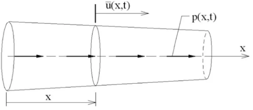
Consider straight bar of length L and variable cross-sectional area A, according to Fig. 1. For simplicity, it is considered that the cross section does not vary abruptly and maintains a constant shape, only by varying its area as a function of the horizontal relative position x. No damping effects are incorporated into this model and the constituent material is considered of linear behavior with modulus of elasticity E being able to vary as a function of x and has specific mass ρ Craig, 1981; Arndt et al., 2010 .
Figure 1: Bar model.
The vibration of the bar is a time dependent problem, and the equation of motion governing this problem is a partial differential equation. The problem is to find the axial displacement u satisfying:
²
( , ) ²
u u
A EA p x t
t x x
r ¶¶ -¶¶ æèççç ¶ ÷¶ ÷÷÷øö= 1
where p is the externally applied axial force per unit length and t is the time. The solution uu x t( , ) must satisfy the boundary and initial conditions defined in the problem.
According to Carey and Oden 1984 , in order to obtain the variational form of a time dependent problem, test functions w w x , independent of t are selected, and the weighted residual method is applied. Then, this procedure results in the following system of differential equations:
Mu+Ku =F 2
where K is the stiffness matrix, u is the vector of displacements, M is the mass matrix, ü is the vector of accelerations and F is the vector of applied forces. The response of the system of equations can be given through the modal coordinates, natural frequencies and vibration modes, or through transient analysis, applying a direct integration method.
To obtain the fundamental vibration modes and frequencies of the problem it is solved the generalized eigenvalues problem given by Bathe, 1996; Hughes, 1987; Zienkiewicz and Taylor, 2000 :
²
KF =wMF 3
where ω are the vibration frequencies andF are the vibration modes of the problem. The stiffness and the mass matrices can be assembled as:
0
i, 1,2, 3... L
j i ij
K EA dx j N
x x f f ¶ ¶ = = ¶ 
0
i, 1,2, 3... L
ij i j
M =
ò
r f fA dx j = N 5where ( )x are the basis functions of the approximation subspace, the indices “i” and “j” respectively refer to the “i-th” and “j-th” basis function relative to the calculation of the element i, j of the corresponding matrix and “N” is the dimension of the approximation space. Different subspaces of approximation are proposed for different methods, such as the Finite Element Method, and the Generalized Finite Element Method.
2.2 Finite Element Method
The standard Finite Element Method uses polynomials shape functions in the approximated solution which can be expressed generally in matrix form as Bathe, 1996; Hughes, 1987 :
e( ) T h
u x =N q 6
where N is the matrix of shape functions and q is the displacement vector. The polynomial functions may be of any order, the simplest being the linear ones. Taking the uniform bar element Figure 1 with one degree of freedom per node, the terms of the approximated solution Equation 6 using linear Lagrangian polynomials as local shape functions are defined in the master element domain[0,1] as
[1 ], T
N = -x x 7
1 2 [u u ],
T
q = 8
, e x L
x = 9
where Le is the element length, and u1 and u2 are the nodal displacements.
2.3 Generalized Finite Element Method
The GFEM is an enriched method of which the main goal is the construction of a finite dimensional subspace of approximating functions using local knowledge about the solution that ensures accurate local and global results. The local enrichment in the approximation subspace is incorporated by the partition of unity approach, which is shown below Melenk and Babuška, 1996; Babuška et al., 2004; Duarte et al., 2000; Piedade Neto and Proença, 2016 .
The approximated solution proposed by the GFEM in the master element domain may be written as the sum of two components:
( )
e e e
h FEM ENRICHED
u x =u +u 10
where e FEM
u is the Finite Element Method component based on nodal degrees of freedom and ueENRICHED is the enriched component by the partition of unity approach based on field degrees of freedom. In this sense, the bar approximated solution on a master element is:
2 2
1 1 1
( ) ( ) ( ) ( ) ( )
l n e
h i i i ij ij ij ij
i i j
u x h xu h x g xa j xb
= = =
é ù
ê ú
= + ê + ú
ê ú
ë û
å
å
å
11 where hiare the partition of unity functions,gij and jij are the enrichment functions, nl is the number of
enrichment layers, ui are the nodal displacements and, aij and bij are the field degrees of freedom related to the
enrichment functions gij and jij, respectively. The term “layer” is adopted herein as a reference to the use of sets
of enrichment functions which must be applied together. Thus, each new level of enrichment works as a new enrichment layer applied at once. For the linear bar element Figure 1 , the partition of unity functions are those given by Equation 7 .
master element. These clouds are written in the element domain as two pairs of sine and cosine functions. The element domain is considered as [0,1].
Sine cloud:
1
2
sin( ) sin( ( 1))
j j
j j
g b x
g b x
=
= - 12
Cosine cloud:
1
2
cos( ) 1 cos( ( 1)) 1
j j
j j
j b x
j b x
=
-= - - 13
where Le is the element length and j jis a hierarchical enrichment parameter proposed by Arndt 2009
with α 1 and with j varying from 1 to the number of enrichment layers nl , such as j 1, 2, … nl.
2.4 Stabilization Strategies 2.4.1 SGFEM-based Stabilization
Stable Generalized Finite Element Method SGFEM was firstly proposed to address numeric conditioning issues of GFEM Babuška and Banerjee, 2012 . This method consists in the application of a subtle modification of enrichment function prior to its inclusion in GFEM approximation space Gupta et al., 2013; Li, 2014; Lins et al. 2015 .
In the SGFEM, the enrichment functions are modified as described in Equation 14 , as presented by Babuška and Banerjee 2012 :
( ) ( ) ( ( )) i x i x Im i x
j =j - j 14
wherei as the i-th stabilized enrichment function,ias the i-th enrichment function andI( ( ))i x as the linear
interpolant of the i-th enrichment function subordinated to supportm.
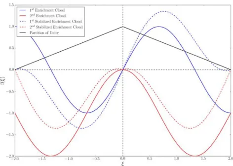
The proposed stabilization of the first layer of enrichment is shown in Figure 2.
2.4.2 Heuristic Modification Stabilization
Note that the variation in the enrichment parameter j implies different characteristics of approaching, as
already pointed out by Arndt 2009 and Torii 2012 . However, the gain in accuracy for certain frequencies does not appear to be associated with numerical stability gain. In fact, apparently there is a certain trade-off between accuracy and numerical stability, regarding the choice of the parameterj.
Since the enrichment parameters jare intrinsically related to the properties of the generated approximation
space, another aspect to be considered relative to these parameters is their construction rule. Thus, a search for better numerical approximation properties, such as stability, should contemplate a study of this aspect. In this context, the proposed modification presented in this paper simply consists of the change in the formation rule of this enrichment parameter.
The choice of this new rule follows an extensive sequence of tests performed for several enrichment parameters and growth rates of these parameters, where it was possible to empirically observe a pattern of minimization of stability problems while maintaining accuracy. This part of the development of the methodology did not result in a general form of representation and therefore the proposal converged to an empirical and heuristic approach that will be explained below.
Recalling that parameter j is calculated by j j, it was proposed a modification, creating new stabilized
parametersj given by:
1
2( 1) 1, 2, 3..., nl
j j j
b
b p
p
é ù
ê ú
= ê - + ú =
ë û 15
It is interesting to note that 11, since:
1 1
1 2(1 1) 0 1
b b
b p p b
p p
é ù é ù
ê ú ê ú
=ê - + ú =ê + ú =
ë û ë û 16
This implies that there is no difference between approximation taken by this approach and the standard trigonometric one for the first layer of enrichment.
3 NUMERICAL RESULTS
In this section modal and transient analysis of bars with polynomial and sinusoidal cross area section variation are presented.
In order to clarify the results presentation, it is necessary to explain some preliminary points.
Firstly, the condition numbers of the matrices are calculated in a classical manner see Wilkinson, 1965 multiplying the norm of the matrix by the norm of its inverse, that is, ( )M M1 M . It is equivalent to divide the greatest eigenvalue by the smallest eigenvalue of the matrix. Conditioning results for stiffness matrices are analogous and mass matrices are adopted for such analysis for its dominant behavior in sensitivity analysis, as highlighted by Petroli et al. 2017 .
As for the enrichment parameter, the 134 value was adopted based on the experience of other works. This value was first used in the Torii’s thesis 2012 . Later, already in the stabilization context, the value of the parameter was again tested in Weinhardt's dissertation Weinhardt, 2016 according to accuracy parameters, resulting in the choice of the 134 value for the following tests. Thus, this enrichment parameter value is adopted for every test result presented in this paper.
3.1 Bar with polynomial cross section area variation
One of the examples of this paper is a bar with polynomial cross area variation modeled as: 4
( ) ( )
A x abx 17
The results for a bar with sinusoidal cross section area variation are presented in the items 3.1.1 and 3.1.2. 3.1.1 Modal Analysis
In order to validate the numerical results, we present the comparison of the numerical values obtained through the exposed methods. Kumar and Sujith 1997 verified that the lower natural frequencies are more affected by the variation of the cross section, and the highest ones are very close to the frequencies of the equivalent uniform bar. Therefore, the results obtained for the first six frequencies of a double-clamped bar with chosen area variation are exposed in the Table 1.
Table 1: Prior Modal Results - Dimensionless Eigenvalues
Vibratio
n mode Analytical Solution
FEM - 100 elements
99 dofs Error
GFEM - 20 elements 1 enrichment
layer 99 dofs
Error
GFEM - 20 elements 2 enrichment
layers 179 dofs
Error
1 3.286007 3.286175 1.680000E-04 3.286008 1.000000E-06 3.286007 0.000000E 00
2 6.360678 6.361800 1.122000E-03 6.360690 1.200000E-05 6.360678 0.000000E 00
3 9.477196 9.480820 3.624000E-03 9.477233 3.700000E-05 9.477196 0.000000E 00
4 12.605890 12.614341 8.451000E-03 12.605973 8.300000E-05 12.605890 0.000000E 00
5 15.739656 15.756038 1.638200E-02 15.739809 1.530000E-04 15.739656 0.000000E 00
6 18.876001 18.904194 2.819300E-02 18.876251 2.500000E-04 18.876001 0.000000E 00
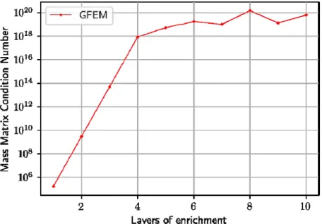
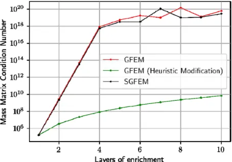
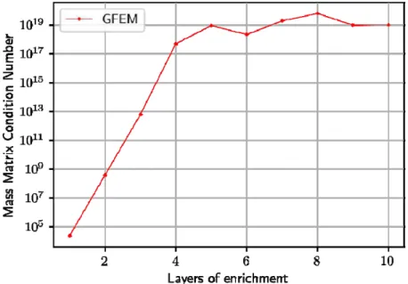
As one may observe in the Table 1, GFEM solution achieve better approximation than FEM using less elements and only one enrichment layer. Applying the second enrichment layer improves even more the accuracy, as shown in the last column of the Table 1. However, the approximation of higher frequencies may require more enrichment layers, as discussed in Weinhardt et al. 2015 and Weinhardt et al. 2017 . This enrichment process may result in numerical instabilities arising from ill-conditioned matrices. The Figure 3 presents the evolution of the condition number of the mass matrix related to a 20-element uniform mesh successively enriched.
Figure 3: Evolution of Mass Matrix Condition Number Numerically Calculated – First example.
3.1.2 Transient Analysis
For the following examples, transient analysis arises in the application of the Newmark Method, as described in Bathe 1996 , using mass and stiffness matrices generated by the application of GFEM with different approaches. Parameters were set such as E c 1
, neglecting damping, and adopting an uniform mesh of 20 finite elements. For the time discretization, the 20 seconds analysis interval was divided in 2000 steps of 10-2 seconds.
The model considered for the examples consists of a bar with a clamped end and the other free end, where the load is applied. Trigonometric enrichment was adopted using 134 due to its performance in modal analysis as presented by Weinhardt et al. 2015 .
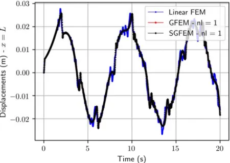
Firstly it is compared an approximation performed using 20-element uniform mesh with: no enrichment FEM ; standard one-layer trigonometric enrichment GFEM ; and Stable one-layer trigonometric enrichment SGFEM . The results are presented in the Figs. 4 and 5, and the external load is applied with a value of 1N in the time range from 0 to 10-2 seconds. It should be noted that, for the first level of enrichment, the Heuristic Modification coincides with the standard GFEM.
Figure 4: Displacements over time.
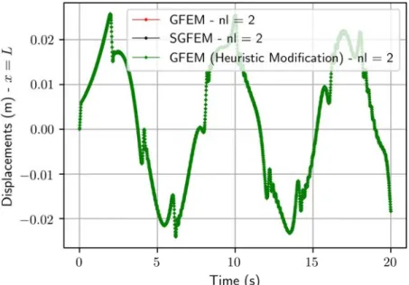
Raising enrichment layer, the results obtained are presented in Figs. 6 and 7 for: GFEM; SGFEM; and Heuristically Modified GFEM.
Figure 6: Displacements over time.
Figure 7: Velocities over time.
Figure 8: Displacements over time.
Figure 9: Velocities over time.
Figure 10: Displacements over time
Figure 11: Velocities over time.
Figure 12: Displacements over time
Figure 13: Velocities over time.
Figure 14: Evolution of Mass Matrix Condition Number Numerically Calculated – First example.
3.2 Bar with sinusoidal cross section area variation
This paper also studied a bar with sinusoidal cross area variation modeled as:
0
( ) sin ²( )
A x =A ax+b 18
where A0,a and b are parameters that describe the sinusoidal variation.
The results for a bar with sinusoidal cross section area variation are presented in the items 3.2.1 and 3.2.2. 3.2.1 Modal Analysis
As in the example 3.1, in order to validate the numerical results, we present the comparison of the numerical solutions obtained through the exposed methods. The results obtained for the first six frequencies of a double-clamped bar with area variation as chosen are exposed in Table 2.
Table 2: Prior Modal Results - Dimensionless Eigenvalues
Vibration
mode Analytical Solution
FEM - 100 elements
99 dofs Error
GFEM - 20 elements 1 enrichment
layer 99 dofs
Error
GFEM - 20 elements 2 enrichment
layers 179 dofs
Error
1 2.978189 2.978330 1.410000E-04 2.978190 1.000000E-06 2.978188 -1.000000E-06
2 6.203097 6.204151 1.054000E-03 6.203108 1.100000E-05 6.203097 0.000000E 00
3 9.371576 9.375094 3.518000E-03 9.371612 3.600000E-05 9.371576 0.000000E 00
4 12.526519 12.534827 8.308000E-03 12.526600 8.100000E-05 12.526519 0.000000E 00
5 15.676100 15.692301 1.620100E-02 15.676252 1.520000E-04 15.676100 0.000000E 00
6 18.823011 18.850986 2.797500E-02 18.823259 2.480000E-04 18.823011 0.000000E 00
Figure 15: Evolution of Mass Matrix Condition Number Numerically Calculated – Second example.
3.2.2 Transient Analysis
As in the previous example, transient analysis arises in the application of the Newmark Method, as described in Bathe 1996 , using mass and stiffness matrices generated by the application of GFEM with different approaches. Parameters were set such as E c 1
, neglecting damping, and adopting a uniform mesh of 20 finite elements. For the time discretization, the 20 seconds analysis interval was divided in 2000 steps of 10-2 seconds.
The model considered for the example consists of a bar with a clamped end and the other free end, where the load is applied. Trigonometric enrichment was adopted using 134 due to its performance in modal analysis as presented by Weinhardt et al. 2015 .
Figure 16: Displacements over time.
Figure 17: Velocities over time.
Figure 18: Displacements over time.
Figure 19: Velocities over time.
Figure 20: Displacements over time.
Figure 21: Velocities over time.
Figure 22: Displacements over time
Figure 23: Velocities over time.
Figure 24: Displacements over time
Figure 25: Velocities over time.
Figure 26: Evolution of Mass Matrix Condition Number Numerically Calculated – Second example.
3.3 Behavior Analysis
The same methodology of numerical experimentation was adopted for both bar examples with variation of polynomial and sinusoidal cross section and the results analysis were described. A central point of this analysis is the observation that although the two examples have different responses and characteristics, the results in terms of the stabilization procedure were similar, which highlights the technique’s robustness in this family of problems. The impulse loading case was studied and responses were presented for displacements and velocities. Acceleration was omitted since it is poorly approximated using continuous functions. Firstly, the approximation was made by one layer of enrichment, concerning GFEM, SGFEM, and FEM. As shown in Figs. 4, 5, 16 and 17, displacements response has large oscillations for Linear FEM and a more accurate behavior for all enriched approaches. On the other hand, the answer in terms of velocities presents great disturbance for the three alternative approaches.
Results for displacements and velocities tend to present more accurate behavior as analytical refinement is performed, as shown in Figs. 6, 7, 18 and 19 for 2 layers and Figs. 8, 9, 20 and 21 for 3 layers of enrichment.
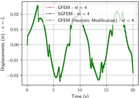
Applying 4 layers of enrichment, GFEM, SGFEM and the Heuristic Modification were compared, as shown in Figs. 10, 11, 22 and 23. The corresponding approximations for displacements are considerably close and more accurate than the previous results, and the Heuristic Modification resulted in a fairly accurate approximation for the first time steps. However, the velocities response for SGFEM presented a pretty deteriorated behavior over time.
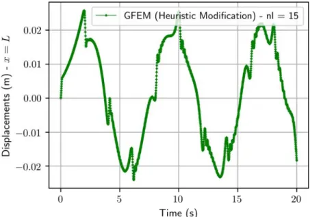
Testing the stability of the proposed Heuristic Modification, Figs. 12, 13, 24 and 25 show the results of application of 15 layers of enrichment. In these examples the high order refinement did not result in significant gains in accuracy for both displacements and velocities. However, it is worth noting that the application of many enrichment layers did not compromised the stability of the Heuristic Modification numerical approach, following the trend shown previously in modal analysis as presented by Weinhardt et al. 2015 , Weinhardt et al. 2016 and Weinhardt et al. 2017 .
4. CONCLUDING REMARKS
This paper discussed issues which are relevant to the stability of the Generalized Finite Element Method applied to dynamic analysis. One-dimensional bars with non-uniform cross area were presented contemplating modal and transient analysis. GFEM formulation with trigonometric enrichment was based on proposals of Arndt
2009 and Torii 2012 .
solution of equation systems by Babuška and Banerjee 2012 . The second proposal was the modification of the parameter βj present in GFEM trigonometric functions enrichment proposed by Arndt 2009 and Torii 2012 .
For transient analysis it was used the Newmark method reusing the already calculated mass and stiffness matrices generated by GFEM. Although the results presented inherent disturbances of Newmark method, it was possible to compare the proposals for approximation among each other, and the second proposal stabilization stood out in most examples. The possibility of making high-order return fines with consequent improvement in response without affecting the CFL stability condition Courant-Friedrichs-Lewy, De Moura and Kubrusly 2012 was presented.
The results of this work point out that there are ways to overcome instability problems in GFEM applied to dynamic analysis, since simple proposals were able to positively impact the approaches.
Additionally, it was possible to observe that the Heuristic Modification stood out in stabilizing the problem, despite the non-uniform cross section. Therefore, it is possible to suppose that stabilization strategies similar to those presented in this paper may be extended to other applications.
References
Aragon, A. M., Duarte, C. A., Gaubelle, P. H. 2010 . Generalized finite element enrichment functions for discontinuous gradient fields. International Journal for Numerical Methods in Engineering 82: 242–268.
Arndt, M. 2009 . The Generalized Finite Element Method applied to free vibration analysis of framed structures. Thesis in Portuguese , Federal University of Paraná, Brazil.
Arndt, M., Machado, R. D., Scremin, A. 2011 . The Generalized Finite Element Method applied to free vibration of framed structures. Advances in Vibration Analysis Research. 187-212.
Arndt, M., Machado, R., and Scremin, A. 2010 . An adaptive Generalized Finite Element Method applied to free vibration analysis of straight bars and trusses. Journal of Sound and Vibration 329 6 : 659–672.
Babuška, I., Banerjee, U., Osborn, J.E. 2004 . Generalized finite element methods: main ideas, results, and perspective. Technical Report No. 04-08, TICAM, University of Texas at Austin, Austin.
Babuška, I.; Caloz, G.; Osborn, J. E. 1994 . Special finite element methods for a class of second order elliptic problems with rough coefficients. SIAM Journal on Numerical Analysis 31 4 : 945-981.
Babuška, I.; Melenk, J. M. 1997 . The partition of unity method. International Journal for Numerical Methods in Engineering 40 4 : 727–758.
Babuška, I. Banerjee, U. 2012 . Stable Generalized Finite Element Method SGFEM . Computer Methods in Applied Mechanics and Engineering 201-204: 91–111.
Bathe, K.-J. 1996 . Finite element procedures. Prentice-Hall.
Belytschko, T.; Black, T. 1999 . Elastic crack growth in finite elements with minimal remeshing. International Journal for Numerical Methods in Engineering 45 5 : 601– 620.
Carey, G. F. and Oden, J. T. 1984 . Finite elements: computational aspects. Prentice Hall.
Craig, R. R. 1981 . Structural dynamics: an introduction to computer methods. John Wiley & Sons Inc.
De Moura, C. A. and Kubrusly, C. S. 2012 . The Courant–Friedrichs–Lewy CFL Condition: 80 years after Its discovery. Springer Science & Business Media.
Duarte, C. A.; Oden, J. T. 1996b . Hp clouds and hp meshless method. Numerical Methods for Partial Differential Equations 12 6 : 673–706.
Duarte, C.A., Babuška, I., Oden, J. T. 2000 . Generalized Finite Element Methods for three dimensional structural mechanics problems. Computers and Structures 77 2 : 215-232.
Fries, T. P. 2008 . A corrected XFEM approximation without problems in blending elements. International Journal for Numerical Methods in Engineering 75 5 :503
Gupta, V., Duarte, C. A., Babuška, I., Banerjee, U. 2013 . A stable and optimally convergent generalized FEM SGFEM for linear elastic fracture mechanics. Computer Methods in Applied Mechanics and Engineering, 266:23– 39
Gupta, V., Duarte, C. A., Babuška, I., Banerjee, U. 2015 . Stable GFEM SGFEM : Improved conditioning and accuracy of GFEM/XFEM for three-dimensional fracture mechanics. Computer Methods in Applied Mechanics and Engineering 289: 355–386.
Hsu, Y. S. 2016 . Enriched Finite Element Methods for Timoshenko beam free vibration analysis. Applied Mathematical Modelling 40 15 : 7012-7033.
Hsu, Y. S.; Machado, R. D.; Abdalla Filho, J. E. . Dynamic analysis of Euler-Bernoulli beam problems using the Generalized Finite Element Method. Computers & Structures, v. 173, p. 109-122, 2016.
Hughes, T.J.R. 1987 . The Finite Element Method: Linear Static and Dynamic Finite Element Analysis. Prentice Hall.
Kumar, B.M. Sujith, R. I. 1997 . Exact solutions for the longitudinal vibration of nonuniform rods. Journal of Sound and Vibration 207 5 : 721-729.
Li, H. 2014 . Investigation of stability and accuracy of high order generalized finite element methods. Thesis, University of Illinois at Urbana-Champaign.
Lins, R., M., Ferreira, M. D. C., Proença, S. P. B., Duarte, C. A. 2015 . An a-posteriori error estimator for linear elastic fracture mechanics using the stable generalized/extended finite element method. Computational Mechanics 56:947-965.
Lu, C., Shanker, B. 2007 . Generalized Finite Element Method for vector electromagnetic problems. Antennas and Propagation, IEEE Transactions 55 5 : 1369–1381.
Melenk, J. M. 1995 . On generalized finite element methods. PhD Dissertation. The University of Maryland.
Melenk, J.M. and Babuška, I. 1996 . The Partition of Unity finite element method: basic theory and applications. Computer Methods in Applied Mechanics and Engineering 139 1-4 : 289-314.
Menk, A., Bordas, S. P. A. 2011 . A robust preconditioning technique for the extended finite element method. International Journal for Numerical Methods in Engineering 85: 1609–1632.
Möes, N.; Dolbow, J.; Belytschko, T. 1999 . A Finite Element Method for crack growth without remeshing. International Journal for Numerical Methods in Engineering 46 1 :131-150.
O’Hara, P., Duarte, C., Eason, T 2009 . Generalized finite element analysis of three-dimensional heat transfer problems exhibiting sharp thermal gradients. Computer Methods in Applied Mechanics and Engineering 198 21 :1857–1871.
Petroli, T., Arndt, M., Machado, R. D., Weinhardt, P. O. 2017 . Numerical stability of GFEM evaluation for free vibration analysis in trussed structures. Proceedings of the 6th International Symposium on Solid Mechanics. Joinville, Brazil 1: 761-775.
Piedade Neto, D., Proença, S. P. B. 2016 . Generalized Finite Element Method in linear and nonlinear structural dynamic analyses. Engineering Computations 33 3 : 806-830.
Sauerland, H., Fries, T. P. 2013 . The stable XFEM for two-phase flows. Computers & Fluids 87: 41–49.
Shang, Y. H. 2014 . Dynamic elastoplastic analysis of solids mechanics problems via enriched finite element methods. Thesis in Portuguese , Pontifical Catholic University of Paraná.
Shibanuma, K., Utsunomiya, T., Aihara, S. 2014 . An explicit application of partition of unity approach to XFEM approximation for precise reproduction of a priori knowledge of solution. International Journal for Numerical Methods in Engineering 97 8 : 551-581.
Sillem, A., Simone, A., Sluys, L. 2015 . The Orthonormalized Generalized Finite Element Method: OGFEM: Efficient and stable reduction of approximation errors through multiple orthonormalized enriched basis functions. Computer Methods in Applied Mechanics and Engineering 287: 112–149.
Torii, A. J. 2012 . Dynamic analysis of structures with the Generalized Finite Element Method. Thesis in Portuguese , Federal University of Paraná.
Torii, A. J.; Machado, R. D. 2012 . Structural dynamic analysis for time response of bars and trusses using the generalized finite element method. Latin American Journal of Solids and Structures 9 3 : 1–31.
Torii, A. J., Machado, R. D., Arndt, M 2016 . GFEM for modal analysis of 2D wave equation. Engineering Computations 32 6 : 1779–1801.
Weinhardt, P. O. 2016 . Study of the Stability of the Generalized Finite Element Method applied to Dynamic Analysis in Portuguese , Federal University of Paraná.
Weinhardt, P. O., Arndt, M., Machado, R. D. 2016 . GFEM stabilization techniques applied to transient dynamic analysis. Revista Interdisciplinar De Pesquisa Em Engenharia 2: 156-170.
Weinhardt, P. O., Debella, L.B.C., Arndt, M., Machado, R. D. 2017 . GFEM Stabilization Techniques Applied to Dynamic Analysis of Non-Uniform Section Bars. Proceedings of the 6th International Symposium on Solid Mechanics. Joinville, Brazil 1:776-789.
Weinhardt, P. O., Rauen, M., Machado, R. D., and Arndt, M. 2015 . Application of the Finite Element Method, Isogeometric Analysis and Enriched Methods to 1D Dynamic Analysis In Portuguese . Proceedings of CMN 2015, Lisboa, Portugal.
Wilkinson, J.H. 1965 . The algebraic eigenvalue problem. Oxford: Clarendon Press.
Yazid, A., Abdelkader, N., Abdelmadjid, H. 2009 . A state-of-the-art review of the x-fem for computational fracture mechanics. Applied Mathematical Modelling 33 2 : 4269– 4282.