Location of Upstream and Downstream Industries

(1)

Carlos Pestana Barros & Nicolas Peypoch

A Comparative Analysis of Productivity Change in Italian and Portuguese Airports

WP 006/2007/DE _________________________________________________________

José Pedro Pontes

Location of Upstream and Downstream Industries

WP 30/2008/DE/UECE _________________________________________________________

Department of Economics

W

ORKING

P

APERS

ISSN Nº0874-4548

School of Economics and Management

(2)

March 2008

Location of upstream and downstream industries

Abstract

This paper studies the issue of agglomeration versus fragmentation of vertically related industries. While the downstream industry works under perfect competition, the upstream industry is a duopoly where each firm supplies a differentiated input to the competitivefirms. These process the inputs under a quadratic production function entailing decreasing returns as in PENG, THISSE and WANG (2006). It is found that fragmentation occurs if the transport cost offinal goods is medium to high, while the transport cost of inputs is low. Otherwise, agglomeration prevails. Multiple agglomerated equilibria are possible if the transport cost of intermediate goods is either medium or high.

Keywords: Oligopoly; Vertically-Linked Firms; Location; Spatial Fragmentation.

J.E.L.Codes: L13; R10.

Author’s Address: ISEG, Rua Miguel Lupi, 20, 1249-078 Lisboa, Portugal. Tel. +351 21 3925916

Fax +351 21 3922808 Email<[email protected]>

(3)

1 Introduction

As AMITI (2005) remarked, the evolution of the location of vertically linked industries exhibits

trends of both clustering and fragmentation. For instance, in the textile sector, manufacturing is

shifted to low labour cost countries, while design and marketing are placed close toﬁnal consumers.

This pattern characterizes a wide range of consumer goods industries.

By contrast, in more technologically industries such as the car, aerospace, pharmaceutical

and electronics, suppliers an buyers of intermediate goods usually stay close in order to save on

transport costs of the inputs, regardless of the labor intensity in their production. In the case of

the car industry, producers of parts often co-locate with assembly plants.

The diﬀerent locational pattern of vertically linked industries can be accounted for by the

diﬀerent transport costs of consumer goods and of intermediate goods. According to PAIS and

PONTES (2008), upstream and downstreamﬁrms locate in low labor cost countries if the transport

costs (both ﬁnal and intermediate) are low. Fragmentation takes place if the transport cost of

intermediate goods is low and the transport cost ofﬁnal goods is medium to high. Agglomeration

in the high labor cost countries occurs if the transport cost of the ﬁnal good is high. Multiple

equilibria (agglomeration of upstream and downstreamﬁrms in either country) take place if both

transport costs are high.

However PAIS and PONTES (2008) assume a very simple vertical structure, based on a

succes-sive monopoly where each ﬁrm produces under aﬁxed proportions, constant returns technology.

In this paper, we introduce a more realistic structure, where a duopoly sells diﬀerentiated inputs

to competitive ﬁrms that produce under a decreasing returns quadratic technology inspired in

PENG, THISSE and WANG (2006).

In section 1, the assumptions and the structure of the game are described. In section 2, the

(4)

2 The model

We assume a spatial economy with two countries: H(ome) and F(oreign). H is a market point of

a consumer good, while F is a low labor cost location. Two upstream ﬁrms (U1 and U2) supply

diﬀerentiated inputs to a consumer good industry under perfect competition. We assume that

this industry is represented by a single competitiveﬁrmD. Thisﬁrm charges a parametric price,

which we assume w.l.g. to be equal to 1.

All transactions of the consumer good are located in a central exchange in country H. If the

downstreamﬁrm locates in F, its price net of transport cost is given by1₋τ, whereτ is the unit

transport cost of the consumer good between H and F.

Firms U1 and U2 use a unit of labour per unit of output. F is a low labor cost location,

so that wF < wH where wF, wH are wage rates. The upstream ﬁrms supply amounts x1, x2

of diﬀerentiated inputs that are transformed in a homogeneous consumer good according to the

following quadratic productionﬁrm inspired in PENG, THISSE and WANG (2006):

Y (x1, x2) =α(x1+x2)− µ

β

2

¶ ¡

x2 1+x

2 2 ¢

−δx1x2 (1)

withα >0, β > δ_≥0. In this setting,β₋δmeasures the degree of sophistication of the productive

process, i.e., the degree of diﬀerentiation of the inputs. The fact that δ is nonnegative implies

that the inputs are substitutes in production. The interregional unit transport cost of the inputs

is expressed byt.

Each upstreamﬁrm charges a fob mill price, so that its proﬁt function is

πi= (pi−wj)xi, i= 1,2;j =H, F (2)

The spatial economy is modelled through a noncooperative game with three stages:

1st Stage FirmsU1, U2 andD select simultaneously locations in{H, F}.

(5)

3rd Stage FirmDselects the amounts to buy of the inputsx1, x2and hence the amount produced

of theﬁnal good.

As usual, the game is solved by backward induction in order to ﬁnd a subgame perfect

equi-librium.

3 Solving the game

In what follows, we solve the 3rd stage and the 2nd stage for each set of locations selected by the

ﬁrms. In order to solve the game quickly, the following parameter speciﬁcations are made:

α = 10, β= 2, δ= 1 (3)

wh = 1, wf = 0

Let(s1, s2_,s_d)be the vector of locations so thats_i (i= 1,2) is the location ofﬁrm U_i ands_d

is the location ofﬁrm D. Then the location subgames are as follows.

3.1 Case

(

H, H, H

)

The proﬁt function of the downstreamﬁrm is

πd=Y −p1x1−p2x2

where Y is given by 1. The proﬁt functions of the upstreamﬁrms are given by

π1 = (p1−w_h)x1 (4)

π2 = (p2−w_h)x2

Maximizing πd with relation to x1, x2, we obtain the demand functions of the inputs by the

downstreamﬁrm (bearing in mind 3):

x1 =

1 3p2−

2 3p1+

10 3

x2 =

1 3p1−

2 3p2+

(6)

Substituting these outputs in 4 and maximizing with relation top1, p2, we obtainp1=p2= 4.

3.2 Case

(

F, H, H

)

πd=Y −(p1+t)x1−p2x2

π1 = (p1−w_f)x1 (5)

π2 = (p2−w_h)x2

x1 =

1 3p2−

2 3p1−

2 3t+

10 3

x2 =

1 3t+

1 3p1−

2 3p2+

10 3

Substituting these outputs in 5 and maximizing with relation top1, p2, we obtain

p1 =

52 15 −

7 15t

p2 =

2 15t+

58 15

3.3 Case

(

H, F, H

)

πd=Y −p1x1−(p2+t)x2

π1 = (p1−w_h)x1 (6)

(7)

x1 =

1 3t−

2 3p1+

1 3p2+

10 3

x2 =

1 3p1−

2 3t−

2 3p2+

10 3

p1 =

2 15t+

58 15

p2 =

52 15 −

7 15t

3.4 Case

(

F, F, H

)

πd=Y −(p1+t)x1−(p2+t)x2

where Y is given by 1. The proﬁt functions of the upstreamﬁrms are

π1 = (p1−w_f)x1 (7)

π2 = (p2−w_f)x2

x1 =

1 3p2−

2 3p1−

1 3t+

10 3

x2 =

1 3p1−

1 3t−

2 3p2+

10 3

p1 =

10 3 −

1 3t

p2 =

10 3 −

(8)

3.5 Case

(

H, H, F

)

πd= (1−τ)Y −(p1+t)x1−(p2+t)x2

π1 = (p1−w_h)x1 (8)

π2 = (p2−w_h)x2

x1 =

1

3τ₋3(t+ 10τ+ 2p1−p2−10)

x2 =

1

3τ−3(t+ 10τ−p1+ 2p2−10)

p1 = 4−

10 3τ−

1 3t

p2 = 4−

10 3τ−

1 3t

3.6 Case

(

F, H, F

)

πd= (1−τ)Y −p1x1−(p2+t)x2

π1 = (p1−w_f)x1 (9)

(9)

Maximizing πd with relation tox1, x2, we obtain the demand functions of the inputs by the

x1 =

1

3τ₋3(10τ−t+ 2p1−p2−10)

x2 =

1

3τ₋3(2t+ 10τ−p1+ 2p2−10)

Substituting these outputs in 9 and maximizing in relation top1, p2, we obtain:

p1 =

2 15t−

10 3τ+

52 15

p2 =

58 15−

10 3 τ−

7 15t

3.7 Case

(

H, F, F

)

πd= (1−τ)Y −(p1+t)x1−p2x2

where Y is given by 1. The proﬁt functions of the upstreamﬁrms are:

π1 = (p1−w_h)x1 (10)

π2 = (p2−w_f)x2

Maximizing πd with relation to x1, x2 we obtain the demand functions of the inputs by the

downstreamﬁrm (bearing in mind 3)

x1 =

1

3τ₋3(2t+ 10τ+ 2p1−p2−10)

x2 =

1

3τ−3(10τ−t1−p1+ 2p2−10)

Substituting these outputs in 10 and maximizing in relation top1, p2 we obtain:

p1 =

58 15−

10 3 τ−

7 15

p2 =

2 15t−

10 3τ+

(10)

3.8 Case

(

F, F, F

)

The proﬁt function of the downstream function is

πd= (1−τ)Y −p1x1−p2x2

π1 = (p1−w_f)x1 (11)

π2 = (p2−w_f)x2

Maximizing the downstream proﬁt function with relation to x1, x2, we obtain the demand

functions of the inputs:

x1 =

1

3τ₋3(10τ+ 2p1−p2−10)

x2 =

1

3τ−3(10τ−p1+ 2p2−10)

Substituting these in 11 and maximizing in relation top1, p2, we obtain the prices

p1 =

10 3 −

10 3τ

p2 =

10 3 −

10 3τ

3.9 Pro

_ﬁ

ts in the

_ﬁ

rst stage game

Pluggingx1, x2, p1, p2 in the proﬁt functions, bearing in mind the production function 1., we can

write the proﬁts in theﬁrst stage game.

Case (H, H, H)

πd = 12

π1 = 6

(11)

Case (F, H, H)

πd =

4 675

¡

13t2

−251t+ 2263¢

π1 =

2

675(7t−52)

2

π2 =

2

675(2t+ 43)

2

Case (H, F, H)

πd = 4

675

¡

13t2

−251t+ 2263¢

π1 =

2

675(2t+ 43)

2

π2 =

2

675(7t−52)

Case (F, F, H)

πd = 4

27(t−10)

2

π1 =

2

27(t−10)

2

π2 =

2

27(t−10)

2

Case (H, H, F)

πd = µ

−₂₇4

¶

(τ₋1)−1(t+ 10τ₋9)2

π1 = µ

−₂₇2

¶

(τ₋1)−1(t+ 10τ₋9)2

π2 = µ

−₂₇2

¶

(τ₋1)−1(t+ 10τ₋9)2

Case (F, H, F)

πd = µ

−₆₇₅4

¶

(τ₋1)−1¡250tτ₋4750τ₋224t+ 13t2

+ 2500τ2

+ 2263¢

π1 = µ

−₆₇₅8

¶

(τ₋1)−1(t₋25τ+ 26)2

π2 = µ

−₆₇₅2

¶

(12)

Case (H, F, F)

πd = µ

−₆₇₅4

¶

(τ₋1)−1¡250tτ₋4750τ₋224t+ 13t2

+ 2500τ2

+ 2263¢

π1 = µ

−₆₇₅2

¶

(τ₋1)−1(7t+ 50τ₋43)2

π2 = µ

−₆₇₅8

¶

(τ₋1)−1(t₋25τ+ 26)2

Case (F, F, F)

πd = µ

−400₂₇ ¶

(τ−1)

π1 = π2= µ

−200₂₇ ¶

(τ₋1)

4 Solving the location game

We consider ﬁrst the truncated 2×2 symmetric game where the downstream ﬁrm locates in

country H. In order to assess the candidates of a locational equilibrium, we calculate a1 anda2,

where

a1 = π1(H, H, H)−π1(F, H, H) (12)

=

µ −₆₇₅14

¶

(t₋1) (7t₋97)

a2 = π1(F, F, H)−π1(H, F, H)

= 14

225(t−1) (t−31)

It is clear from 12 that:

                      

a1<0∧a2>0 ift <1 F is a dominant strategy

a1>0∧a2<0 if1< t < 97

7 H is a dominant strategy

a1<0∧a2<0 if 97

3 < t <31

There are two asymmetric Nash equilibria(H, F)

and (F, H)

(13)

F. Again we computea1 anda2such that

a1 = π1(H, H, F)−π1(F, H, F) (13)

=

µ −₆₇₅14

¶

(τ−1)−1(3t+ 100τ−97) (t+ 1)

a2 = π1(F, F, F)−π1(H, F, F)

= 14

675(τ−1)

−1

(7t+ 100τ−93) (t+ 1)

It is clear from 13 thata1<0∧a2>0for allt, so thatF is a dominant strategy. Hence the

candidates to equilibrium in the game with three players are:

              

(F, F, H) if t <1

(H, H, H) if t >1

(F, F, F) for allt

We check now whether these proﬁles of strategies are indeed Nash equilibria in the location

game, i.e., whether they are robust to deviations by the downstream ﬁrm. The no-deviation

conditions are:

πd(F, F, H) > πd(F, F, F)⇔t <10−10√1−τ (14)

πd(F, F, F) > πd(F, F, H)⇔t >10−10√1−τ

πd(H, H, H) > πd(H, H, F)⇔t >−10τ−9

√

1₋τ+ 9

The last condition in 14 is always met since₋10τ₋9√1₋τ+ 9is negative forτ_∈[0,1]. A

suﬃcient condition so that the output of the downstreamﬁrm is non-negative is

x2(F, H, F)≥0⇔t≤

43 7 −

50

7τ (15)

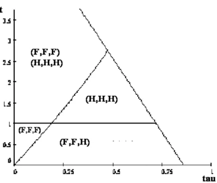
In Figure 1, we plot in(τ , t)space the following expressions:

t = 10₋10√1₋τ

t = 1

t = 43 7 −

(14)

Figure 1: Location regions in(τ , t)space.

5 Concluding remarks

Figure 1 shows that all location equilibria entail the agglomeration of both upstream ﬁrms in the

same country. This follows from the fact that the market for theﬁnal good is located in a single

region. Agglomeration of allﬁrms occurs in country F if both transport costs,tandτ ,are low, so

that locations are driven by labor cost considerations only, apart from considerations related with

access to market. By contrast, agglomeration takes place in region H ifτis high andtis medium.

In this case, location of all ﬁrms is driven towards the location of the market for the consumer

good.

Two special cases are of interest. Theﬁrst one entails spatial fragmentation, the downstream

ﬁrm being located close to the consumer good market in H while the upstream ﬁrms locate in

the low labor cost country F. Unsurprisingly, fragmentation arises if tis low and τ is medium to

(15)

in country H or in country F. This case arises if the transport cost of the inputs is high, so that

every cluster of locations is an equilibrium.

Hence, we can conclude that the location of vertically-linked ﬁrms is completely determined

by the transport costs of the inputs and of the ﬁnal good. We hope that this result, that was

reached through a numeric simulation, can generalized to a wider setting.

References

PAIS, Joana and José Pedro PONTES (2008), "Fragmentation and clustering in vertically-linked industries",Journal of Regional Science,forthcoming.

AMITI, Mary (2005), "location of vertically-linked industries: agglomeration versus com-parative advantage",European Economic Review, 49, 809-832.