Input Specificity and Location

José Pedro Pontes

February 2005

Abstract

In a two-region economy, two upstreamfirms supply an input to two consumer goods firms. For two different location patterns (site specificity and co-location of the suppliers), the firms play a three-stage game: the input suppliers select transport rates; then they choose outputs;finally the buyers select quantities of the consumer good. It is concluded that the site specificity of the input leads to a high transport cost and to its specialized adaptation to the needs of the local user.

K eyw ords: Technological Choice; Spatial Oligop oly; Vertically-linked Industries. JE L classification : D43; R12.

Author’s affiliation: Instituto Sup erior de Economia e Gestão, Technical University of Lisb on and

Research Unit on Complexity in Economics (UECE).

Address: Instituto Sup erior de Economia e Gestão, Rua M iguel Lupi, 20, 1249-078 Lisb oa, Portugal.

Telephone: 351 21 3925916

Fax: 351 21 3922808

Em ail<pp ontes@iseg.utl.pt>

The author wishes to thank Armando Pires and Cristina Albuquerque for their helpful comments.

1. Introduction

The issue of input specificity arises when two industries are vertically linked.

We assume that a set of upstream firms supplies an input to an equal number

of downstream firms. Each downstream firm produces a differentiated consumer

good and uses a differentiated intermediate good. Then each input supplier faces

the following choice. It can either produce an input that is specially adapted to

the requirements of a given buyer, or it can produce a generic or standardized

intermediate good that can be used without much penalty by downstream firms

other than the intended buyer.

This issue is important for several reasons. Firstly, it entails a technological

trade-off. As was acknowledged by RIORDAN and WILLIAMSON (1985),

spe-cialization of the input reduces the marginal production cost of the buying firm,

although it determines a different cost directly related with the level of input

specificity. As McLAREN (2000) remarked, this cost has to do with the difficult

adaptation of the specialized input to the needs of downstream firms other than

the intended buyer.

Secondly, input specialization can lead to inequalities among downstreamfirms.

If most upstreamfirms specialize their inputs to a subset of consumer goodsfirms,

the remaining buying firms will have to incur adaptation costs of the input that

will lead them to produce a smaller amount of output.

Thirdly, input specificity can lead to vertical integration. This can occur for

two different reasons. The specialization of the input creates an incentive for the

continuation in time of a relationship between the seller and the buyer of the input.

relation-ship through common property instead of a market arrangement (RIORDAN and

WILLIAMSON, 1985). This can be seen in terms of a bilateral relationship

be-tween a seller and a buyer, or in the context of the interdependence of the

integra-tion decisions taken by several upstream and downstreamfirms in vertically-linked

industries (McLAREN, 2000; GROSSMAN and HELPMAN, 2002). But vertical

integration can also occur for strategic reasons. An upstream firm can decide to

adapt the input to the requirements of a given buyer. By doing so, it undertakes

not to supply the input to other downstream firms, thus raising their costs. This

benefits the downstreamfirm that buys the specialized input, and this externality

can be internalized if the upstream firm merges with the targeted input buyer

(CHOI and YI, 2000; CHURCH and GANDAL, 2000).

In this paper, the issue of vertical integration will be left to one side and the

focus of our attention will be on the technological aspects of the decision to

spe-cialize in terms of input. Just as HOTELLING (1929) and D’ASPREMONT,

GABSZWICZ and THISSE (1979) did for the horizontal differentiation of a

con-sumer good, input specificity will be modelled as following from "site specificity".

JOSKOW (1987) defined the site specificity of an input through two

complemen-tary causes: (1) the upstream and the downstreamfirms are co-located or (2) the

average distances and the unit transport costs among the buyers and the sellers

are high.

HELSLEY and STRANGE (2004) related the site specificity of an input to

"market thickness". As the number of downstream firms increases, the average

distance between each input supplier and each input buyer decreases. The

agglom-eration offirms decreases input specificity. Site specificity can also be modelled by

(2002), where each downstream firm uses a differentiated input with an address

within a certain circumference. Each input supplier is defined by a location inside

the circle with two coordinates, defined by the radius that joins the location to

the center of the circle and to a point on the circumference. This point on the

circumference defines the differentiated input in which the upstreamfirm is

rela-tively specialized. The distance between the location and the center of the circle

measures the degree of specialization.

In this paper, we will try to relate location and transport costs as causes of

the site specificity of an input. We will follow the approach of the Launhardt

model that was presented by DOS SANTOS FERREIRA and THISSE (1996): for

different location patterns, thefirmsfirst choose transport rates endogenously and

then they compete in the product market. Our approach is also closely related

with DOS SANTOS FERREIRA and ZUSCOVITCH (1995). Eachfirm can choose

between manufacturing a "light" (flexible) product at a high production cost, or a

"heavy" (specialized) product with a low production cost but a high transport cost

(adaptation cost), which the firm must incur if it sells the product in a different

location (to a different buyer). As ANDERSON and DE PALMA (1996) remarked,

this choice amounts to an option for the input supplier between competing locally,

i.e. mainly serving a local buyer, and competing globally, where the firm aims to

supply clients in different locations.

Three main findings follow from our analysis. The first is that the location

and transport cost factors of site specificity are closely related. Firms will be

more likely to produce "heavy" inputs if they are co-located with their buyers

than otherwise. In each case, transport costs will be higher when the returns to

for moderate returns to specialization there will be multiple equilibria in transport

rates, while there will be a single equilibrium for extreme values. The third is that

the intermediate equilibria will be symmetric in the event of the co-location of

input suppliers and buyers and asymmetric if the upstream firms cluster in one

location. This result is reminiscent of DOS SANTOS FERREIRA and THISSE

(1996).

In section 2. the model is presented. In subsection 2.1. the assumptions are

de-fined and the game structure is described. In subsection 2.2. the case is presented

where each upstreamfirm locates separately with each downstreamfirm. In

sub-section 2.3. the other polar case is presented where the input suppliers co-locate.

The conclusions are drawn in section 3..

2. The model

2.1. Assumptions and game structure

The model describes a spatial economy that obeys the following assumptions:

1. The economy is composed of two regions, A and B, each with the same

number n of consumers. Through normalization, we have n = 1. The

distance between the regions,δ, is also normalized toδ= 1.

2. Each consumer has an inverse linear demand function p=a₋bx. For the

sake of simplicity, it will be assumed thata=b= 1.

3. Two downstream firms, D₁ in region A, and D₂ in region B, produce a

homogenous consumer good under local monopoly. The consumer good is

that, for each downstreamfirm, it is more profitable to charge the monopoly

price than to undercut the competitor.

4. Each downstreamfirm uses one unit of an input in order to produce one unit

of thefinal good. The input price is the only marginal production cost of

the downstreamfirm, which does not incur anyfixed costs.

5. Two upstream firms, U1 and U2, produce and deliver a homogeneous

in-termediate good to the final producers, D1 and D2. The upstream firms

compete in quantities sold to each downstreamfirm.

6. Each upstreamfirmUi(i= 1,2)chooses its transport ratetiin the distance

between the regions. The marginal production cost of the input is a

de-creasing function of the transport rate, so that the production of a "lighter"

input entails a higher marginal production cost. The input supplier trades off

the spatialflexibility of the intermediate good against productive efficiency.

The relationship is linear, so that the marginal production cost of the input

produced byfirmUi is given by

ci=α−βti

where

ti ∈ ·

0,α β

¸

α _∈ (0,1)

Figure 1: The case of site specificity

ti∈ h

0,α β i

means that the transport cost and the production cost can take zero

values, which is not realistic, but is admitted for the sake of simplicity. α_∈(0,1)

ensures that the production cost does not exceed each consumer’s reservation

price (equal to 1, according to assumption 2). β _∈ (0,1) ensures that the total

marginal cost (production plus transport) of each upstream firm in the distant

market increases with the transport rate.

With these assumptions, a noncooperative game with three stages is

mod-elled. This game is inspired by the case of vertically-linked industries in a

succes-sive Cournot oligopoly, where firmsfirst select the kind of product differentiation

for given values of the adaptation costs of the inputs, as presented in

BELLE-FLAMME and TOULEMONDE (2003). However, in our game, the locations of

the firms are assumed to be given and the transport rates are endogenous. Two

different patterns of locations of the upstreamfirms are considered and compared:

"site specificity", where each upstream firm locates alongside a different input

buyer (see Figure 1); and "co-location", where both upstreamfirms cluster close

to the same downstreamfirm (see Figure 2).

Figure 2: Co-location of input suppliers

First Stage : FirmsU₁andU₂select the transport rates t₁ andt₂.

Second Stage : FirmU₁chooses the quantitiesq1aandq1band FirmU₂chooses

the quantitiesq2aandq2bof the intermediate good to be sold to the

down-streamfirms in regionsA andB.

Third Stage : DownstreamfirmsD₁ andD₂choose quantities of the consumer

goodx1andx2 to be sold in regionsAandB respectively.

2.2. The case of the site specificity of the input

In this case, it is assumed that each upstream firm locates in a different

re-gion alongside a consumer good producer (see Figure 1) This corresponds to the

Williamsonian concept of the "site specificity" of an asset. It will be shown that

this kind of site specificity implies a specialized adaptation of the input to the

needs of the local buyer, in the sense that the upstreamfirm willfind it profitable

to produce a "heavy" input at a low production cost and sell it to the local buying

firm.

We seek to solve the three-stage game by backward induction in order tofind

third stage are:

πD₁ (x₁,wa) = [(1₋x₁)₋wa]x₁ (1)

πD

2 (x2,wb) = [(1−x2)−wb]x2 (2)

wherewaandwbare the delivered prices of the input in regionsAandB. If these

profit functions are maximized in relation tox₁andx₂, we obtain

x∗₁ = 1

2(1−wa) (3)

x∗₂ = 1

2(1−wb) (4)

In the second stage, letq1a,q1b,q2a,q2b be the quantities of the input sold

by the upstream firms U1 and U2 to the downstream firms in regions A andB.

Then the derived demand of the input in each region is given by the equalities

q1a + q2a = x∗₁=1

2(1−wa) (5)

q1b + q2b = x∗₂=1

2(1−wb) (6)

If these equalities are solved in relation to waand wb, we obtain inverse

de-mands for the input in each region:

wa = 1₋2 (q1a + q2a) (7)

The profit functions firmU₁ andfirm U₂ are:

πU₁ (q1a,q1b,q2a,q2b, t₁) = [wa₋(α₋βt₁)] q1a + [wb₋t₁₋(α₋βt₁)] q1b

(9)

πU₂ (q1a,q1b,q2a,q2b, t2) = [wa−t2−(α−βt2)] q2a + [wb−(α−βt2)] q2b

(10)

where wa and wb are defined by 7 and 8. The Cournot equilibrium outputs in

the second stage of the game follow easily:

∗

q1a (t1, t2) =

1 6t2−

1 6α+

1 3βt1−

1 6βt2+

1

6 (11)

∗

q1b (t1, t2) =

1 3βt1−

1 3t1−

1 6α−

1 6βt2+

1 6 ∗

q2a (t1, t2) =

1 3βt2−

1 3t2−

1 6βt1−

1 6α+

1 6 ∗

q2b (t1, t2) =

1 6t1−

1 6α−

1 6βt1+

1 3βt2+

1 6

We will assume henceforth that these outputs are positive for any values of the

transport rates. It is shown in the Appendix that a sufficient condition for this to

be satisfied is that

α_≤β

2 (12)

This condition means that the marginal production cost of each upstreamfirm

should be sensitive enough to the variation of its transport rate.

functions of the input suppliers in thefirst-stage game.

πU₁ (t₁, t₂) = 1 9t2−

2 9t1−

2 9α+

2 9αt1−

1 9αt2+

4 9βt1−

2 9βt2− −4₉αβt₁+2

9αβt2+ 4 9βt1t2+

1 9α

2₊2

9t 2 1 +1 18t 2 2− 4 9βt 2 1− 1 9βt 2 2+ 4 9β

2_t2 1+

1 9β

2_t2 2+ 1 9− 4 9β 2_t 1t2

(13)

πU₂ (t1, t2) =

1 9t1−

2 9α−

2 9t2−

1 9αt1+

2 9αt2−

2 9βt1+

4 9βt2+

2 9αβt1− −4₉αβt2+

4 9βt1t2+

1 9α

2₊ 1

18t 2 1+ 2 9t 2 2− 1 9βt 2 1− 4 9βt 2 2−

−4₉β2t1t2+

1 9β

2_t2 1+

4 9β

2_t2 2+

1 9

(14)

The second partial derivative of the profit function of each upstream firm in

relation to its own transport rate is given by

∂2_πU i (t1, t2)

∂t2

i

= 4 9−

8

9β(1−β) (15)

fori= 1,2. It can be easily seen that the second partial derivative 15 is positive for

β_∈(0,1), thus ensuring that the profit function of each upstream firm is strictly

convex in its transport rate. Hence the profit function of each input supplier

reaches its maximum value at a boundary point of the domain

·

0,α β

¸

, so that

there are four candidates for a subgame perfect equilibrium in transport rates: two

symmetric equilibria(0,0),³α_β,α_β´; and two asymmetric equilibria³0,α_β´,³α_β,0´.

Since the game is symmetric, it is sufficient to explicitly consider only one of these

(t∗

1, t∗2) = (0,0) is a Nash equilibrium of thefirst-stage game if and only if:

πU₁ (0,0) _≥ πU₁

µ

α β,0

¶

πU₂ (0,0) ≥ πU₂

µ

0,α β

¶

Following 13 and 14, these conditions are both equivalent to

α≤ β(1₁−2β)

−β (16)

On the other hand,(t∗

1, t∗2) =

³ α β,αβ

´

is a Nash equilibrium of the first-stage

game if and only if

πU₁

µ α β, α β ¶

≥ πU₁

µ

0,α β

¶

πU₂

µ α β, α β ¶

≥ πU₂

µ

α β,0

¶

These conditions are equivalent to

α_≥ β(2β−1)

2β2_−β−1 (17)

Finally, the asymmetric equilibrium(t∗₁, t∗₂) =³0,α_β´holds if and only if

πU₁

µ

0,α β

¶

≥ πU₁

µ α β, α β ¶

⇔α≤ β(2β−1) 2β2_−β−1

πU₂

µ

0,α β

¶

≥ πU₂ (0,0)⇔α≥β(1₁−2β)

−β (18)

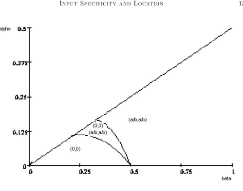
By plotting 12, 16 and 17 together in the(α, β)space, it is possible to define

Figure 3: Equilibria in transport rates in the site specificity case

conditions 18 are incompatible, so that asymmetric equilibria do not exist.

Figure 3 shows that equilibrium transport rates are minimal when the

para-metersαandβare small and that they are maximal otherwise. For intermediate

values of the parameters, both symmetric equilibria coexist. Basically, the

equilib-rium with high transport rates occurs if the returns to specialization of the input

(as measured by β) are high.

2.3. The case of co-location of the input suppliers

Let us assume now that the input suppliers are clustered in regionA, so that

the spatial pattern of the economy is as described by Figure 2. In this case, the

Solving the game by backward induction, it is clear that the third-stage game

is identical to the one that was described in subsection 2.2., so that the profit

functions of the downstream firms are given by 1 and by 2 and the equilibrium

outputs of the consumer good are expressed by 3 and 4.

In the second stage, the inverse demand functions of the input in the two

regions are still given by 7 and 8. But the profit functions of the upstreamfirms

now become

πU

1 (q1a,q1b,q2a,q2b, t1) = [wa−(α−βt1)] q1a + [wb−t1−(α−βt1)] q1b

(19)

πU₂ (q1a,q1b,q2a,q2b, t₂) = [wa₋(α₋βt₂)] q2a + [wb₋t₂₋(α₋βt₂)] q2b

(20)

The equilibrium outputs of the upstreamfirms in the second-stage game

be-come

∗

q1a (t₁, t₂) = 1 3βt1−

1 6α−

1 6βt2+

1

6 (21)

∗

q1b (t₁, t₂) = 1 6t2−

1 3t1−

1 6α+

1 3βt1−

1 6βt2+

1 6 ∗

q2a (t₁, t₂) = 1 3βt2−

1 6βt1−

1 6α+

1 6 ∗

q2b (t₁, t₂) = 1 6t1−

1 6α−

1 3t2−

1 6βt1+

1 3βt2+

1 6

profit functions in the first-stage game.

πU₁ (t₁, t₂) = 1 9t2−

2 9t1−

2 9α+

2 9αt1−

1 9αt2+

4 9βt1−

2 9βt2− −2₉t₁t₂₋4

9αβt1+ 2 9αβt2+

4 9βt1t2+

1 9α

2₊2

9t 2 1+ 1 18t 2 2−

−4₉βt2 1− 1 9βt 2 2− 4 9β 2_t 1t2+

4 9β

2_t2 1+

1 9β

2_t2 2+

1 9

(22)

πU₂ (t1, t2) =

1 9t1−

2 9α−

2 9t2−

1 9αt1+

2 9αt2−

2 9βt1+

4 9βt2− −2₉t1t2+

2 9αβt1−

4 9αβt2+

4 9βt1t2+

1 9α

2₊ 1

18t 2 1+ +2 9t 2 2− 1 9βt 2 1− 4 9βt 2 2− 4 9β 2_t 1t2+

1 9β

2_t2 1+

4 9β

2_t2 2+

1 9

(23)

If we compute the second partial derivatives of the profit functions of the input

suppliers in relation to their own transport cost rates, we conclude that they are

still given by 15, so that each profit function is convex in its own transport rate.

Hence the equilibrium transport rate of eachfirm will necessarily be a boundary

point ofh0,α β i

. In what follows, we check the possible Nash equilibria in transport

rates.

Clearly, there will be a Nash equilibrium(0,0)if and only if

πU₁ (0,0) _≥ πU₁

µ

α β,0

¶

πU₂ (0,0) _≥ πU₂

µ

0,α β

¶

These conditions are equivalent to

α≤ β(1₁−2β)

which is the same as 16.

On the other hand,³α β,αβ

´

will be a Nash equilibrium in thefirst-stage game

if and only if

πU₁

µ α β, α β ¶

≥ πU₁

µ

0,α β

¶

πU₂

µ α β, α β ¶

≥ πU₂

µ

α β,0

¶

These conditions are equivalent to

β_≥ 1

2 (25)

Finally, an asymmetric equilibrium³α β,0

´

exists if and only if

πU₁

µ

α β,0

¶

≥ πU₁ (0,0)

πU₂

µ

α β,0

¶

≥ πU₂

µ α β, α β ¶

which are equivalent to _    

α_≥ β(1−2β) 1−β β_≤1

2

(26)

Conditions 24, 25 and 26 are plotted in Figure 4.

Comparing Figure 4 with Figure 3, it is clear that, as in the case of site

speci-ficity, in the case of co-location of the suppliers, the equilibrium transport rates

will be maximal if the returns to specialization (as measured byβ) are high and

they will be minimal if these returns are low. However, there are differences

smaller in the case of co-location of suppliers when compared with the case of site

specificity. Secondly, for intermediate values of β, we now have multiple

asym-metric equilibria instead of multiple symasym-metric equilibria. In this case, one of the

upstream firms chooses to basically supply the local buyer, while the other one

selects a low transport rate in order to serve downstreamfirms in both regions.

3. Concluding remarks

The analysis has enabled us to draw several conclusions. Thefirst, unsurprising

finding is that specialization occurs if its returns in terms of production cost

reduc-tion are high. This is more likely to occur if each upstreamfirm is close to a buyer

than if they cluster in one single location. The second conclusion is that there

will be one single equilibrium in transport rates if the returns to specialization are

extreme (either too low or too high), but there will be multiple equilibria if these

returns are intermediate. In this case, the multiple equilibria will be symmetric

in the case of site specificity, but asymmetric in the case of co-location of input

suppliers. Finally, while the output of the consumer good will be the same in both

regions in the case of site specificity, it will be different in the case of co-location

of input suppliers. In this latter case, the output of the consumer good is higher

in the region where the input suppliers are located, if at least one of the upstream

firms specializes its intermediate good. These conclusions are reminiscent of

(al-though not entirely coincident) DOS SANTOS FERREIRA and THISSE (1996).

The conclusions can be summarized by saying that the site specificity of the input,

following from the joint location of an upstream and a downstreamfirm, leads to

its specialization as a result of the choice of high transport rates by the suppliers.

Thefirst one is the endogenisation of the location choice made by thefirms, which

determines the degree of input specificity. If this is done, it becomes necessary to

explain why the upstreamfirms may co-locate, by means of some kind of

agglomer-ation economy. The second extension would be to consider different values for the

distance between the regions,δ, instead of a single value. Following ANDERSON

and DE PALMA (1996), it is expected that a high value ofδwill by itself lead to

a higher degree of localization of competition in the input market and to a higher

input specificity.

Appendix: Derivation of conditionα_≤ β 2.

We dealfirst with the case of site specificity presented in subsection 2.2.. From

11, it is clear that q1b (t₁, t₂)_≥0and q2a (t₁, t₂)_≥0are equivalent respectively

to

t1 ≤

α+βt2−1

2β₋2 (A.1)

t_{2 ≤} α+βt1−1 2β−2

If the relations A.1 are taken as equalities, they define two decreasing functions

in the space(t₁, t₂), which intersect at

t∗₁=t∗₂=1−α

2₋β (A.2)

Clearly, a sufficient condition for each upstreamfirm to be active in its distant

firm, is that its transport rate does not exceed A.2, i.e.

α β ≤

1₋α 2₋β

which is equivalent toα_≤ β 2.

Then the case of co-location of the input suppliers, which is dealt with in

subsec-tion 2.3., is examined. From 21, it is clear thatq1b (t1, t2)≥0andq2b (t1, t2)≥0

mean respectively that

t1 ≤

α₋t₂+βt₂₋1

2β−2 (A.3)

t_{2 ≤} α−t1+βt1−1 2β₋2

If relations A.3 are met as equalities, they define two increasing functions. The

intercept of each function in its axis is given by

t∗₁=t∗₂= 1−α

2 (1₋β) (A.4)

Clearly, a sufficient condition for each upstreamfirm to be active in the distant

marketB, for any transport rate that may be selected by the competitor, is that

its transport rate does not exceed A.4, or

α β ≤

1₋α 2 (1₋β)

which is equivalent to

α≤₂β

−β (A.5)

each upstreamfirm to be active in its distant market for any transport rate that

may be selected by the competitor.

References

ANDERSON, Simon and Andre DE PALMA (1996), "From local to global

com-petition", CEPR Discussion Paper, January.

BELLEFLAMME, Paul and Eric TOULEMONDE (2003), "Product diff

erentia-tion in successive vertical oligopolies",Canadian Journal of Economics, 36(3),

pp. 523-545.

CHOI, Jay Pil and Sang-Seung YI (2000), "Vertical foreclosure with the choice of

input specifications",RAND Journal of Economics, 31(4), Winter, pp. 717-743.

CHURCH, Jeffrey and Neil GANDAL (2000), "Systems competition, vertical

merger and foreclosure",Journal of Economics & Management Strategy, 9(1),

Spring, pp. 25-51.

D’ASPREMONT, Claude, Jean GABSZEWICZ and Jacques-François THISSE

(1979), "On Hotelling’s ’Stability in Competition’",Econometrica, 47(5),

Sep-tember, pp. 1145-1150.

DOS SANTOS FERREIRA, Rodolphe and Ehud ZUSCOVITCH (1995), "A model

of technological choice: the specialization-flexibility trade-off", BETA,

Univer-sité Louis Pasteur, processed.

DOS SANTOS FERREIRA, Rodolphe and Jacques-François THISSE (1996),

"Horizontal and vertical differentiation — the Launhardt model",International

GROSSMAN, Gene M. and Elhanan HELPMAN (2002), "Integration versus

out-sourcing in industry equilibrium",Quarterly Journal of Economics, 117(1), pp.

85-120.

HELSLEY, Robert and William STRANGE (2004), "Agglomeration, opportunism

and the organization of production", processed.

HOTELLING, Harold (1929), "Stability in competition", Economic Journal,

39(154), pp. 41-57.

JOSKOW, Paul (1987), "Contract duration and relation-specific investments:

em-pirical evidence from coal markets",American Economic Review, 77(1), March,

pp. 168-185.

McLAREN, John (2000), "’Globalization’ and vertical structure", American

Eco-nomic Review, 90(5), December, pp. 1239-1254.

RIORDAN, Michael and Oliver WILLIAMSON (1985), "Asset specificity and

eco-nomic organization",International Journal of Industrial Organization, 3, pp.