Carlos Pestana Barros & Nicolas Peypoch
A Comparative Analysis of Productivity Change in Italian and Portuguese Airports
WP 006/2007/DE _________________________________________________________
Paulo Brito, Luís Costa & Huw Dixon
Non-Smooth Dynamics and Multiple Equilibria in a
Cournt-Ramsey Model with Endogenous Markups
WP 14/2010/DE/UECE _________________________________________________________
Department of Economics
W
ORKINGP
APERSISSN Nº 0874-4548
School of Economics and Management
Non-smooth Dynamics and Multiple Equilibria in a
Cournot-Ramsey Model with Endogenous Markups
✩Paulo B. Britoa, Lu´ıs F. Costaa, Huw Dixonb,∗
a
ISEG (School of Economics and Management) Technical University of Lisbon and UECE (Research Unit on Complexity and Economics), Rua do Quelhas 6, 1200-781 Lisboa, Portugal.
b
Cardiff Business School, Aberconway Building, Column Drive, Cardiff, CF10 3EU, United Kingdom.
Abstract
We consider a Ramsey model with a continuum of Cournotian industries where free entry generates an endogenous markup. The model produces two different regimes, monopoly and oligopoly, resulting in non-smooth dynamics. We analyze the global dynamics of the model, demonstrating the model may exhibit heteroclinic orbits connecting multiple equi-libria. Small transitory changes in parameters can lead to large permanent effects and there can be a Rostovian poverty trap separating a low-capital and high-markup equilibrium from a high-capital low-markup equilibrium. The paper applies recent results from applied math-ematics for non-smooth dynamic systems.
Keywords: Endogenous markups, Non-smooth dynamics, Discontinuity induced
bifurcations, Heteroclinic orbits.
JEL codes: C62, D43, E32
✩Financial support by FCT is gratefully acknowledged. This article is part of project
POCTI/ECO/46580/2002 which is co-funded by ERDF. We are grateful to Guido Ascari, Jean-Pascal B´enassy, Stefano Bosi, Rodolphe dos Santos Ferreira, Gianluca Femminis, Jean-Michel Grandmont, Teresa Lloyd Braga, Thomas Seegmuller, Peter Simmons, Gabriel Talmain, Alain Venditti, to the participants at the 21st Annual Congress of the European Economic Association (Vienna), at the 38th Conference of the Money Macro and Finance Research Group (York), at the ASSET Annual Meeting (Lisbon), at the 2nd Annual Meeting of the Portuguese Economic Journal (´Evora), at the Anglo-French-Italian Workshop in Macroeco-nomics (Pavia), and at seminars at ISEG/TULisbon, Paris School of EcoMacroeco-nomics, and at the University of York. Faults, off course, remain our own.
∗Corresponding author
Email addresses: [email protected](Paulo B. Brito),[email protected](Lu´ıs F. Costa ),
1. Introduction
Traditionally, the study of differential equations has been based on the assumption of continuous differentiability of at least the first and second order, resulting in smooth dy-namics. Furthermore, in economics most dynamic systems are restricted to a unique stable steady-state equilibrium. In this paper, we take the analysis of dynamic systems in eco-nomics beyond both of these boundaries in developing a model of entry in Cournot product markets (resulting in an endogenous markup) in a dynamic general equilibrium continuous time Ramsey model. Cournot competition has the attraction that increases in economic ac-tivity are associated with more firms and hence lower markups, which captures the empirical feature of counter-cyclical markups - seeinter aliaMartins and Scarpetta (2002). We embed this entry process into an otherwise fairly standard intertemporal representative-household macromodel. The Ramsey household consumes and accumulates capital. Free entry drives profits in each instant to zero, leading to an endogenous markup and hence a wedge be-tween the marginal product and the marginal revenue os capital. We apply recent advances in applied mathematics (Leine (2006), di Bernardo et al. (2008)) which extend traditional analysis to allow for non-smooth piecewise continuous dynamic systems. Furthermore, we develop a comprehensive analysis of the local and global dynamics of an economic system which possesses up to three steady-state equilibria, including up to two saddle-path stable equilibria, and perform the corresponding bifurcation analysis.
Cournotian approach of this paper is the Linneman (2001) model of entry in monopolistic competition as used in Jaimovich (2007) and Jaimovich and Floetotto (2008), and Bilbiie et al. (2007). Entry reduces the market share of firms, and hence reduces the ”own price effect” of the monopolist on the aggregate price index, which increases the elasticity of demand (see Yang and Heidra (1993))1.
Whilst we allow for entry and exit, we place a lower bound on the measure of firms at unity. This eliminates the undesirable property of Cournot entry that the markup can go to unity and hence the marginal revenue product of capital to zero as the ”number” of firms gets below unity and falls towards zero2. In a symmetric Cournot equilibrium, the firm’s
elasticity of demand is the product of the number of firmsnand the industry elasticityσ,nσ
hence when n= 1/σ, the firm’s elasticity is unity so that the equilibrium output is zero and the economy ceases to produce output or accumulate capital3. Whilst placing a lower bound
on the number of firms in an industry avoids this absurd outcome, it creates adiscontinuity
in the dynamic system, since when the number of firms falls to one, the markup remains constant at σ, and the number of industries shrinks. The typical industry in the economy can thus be in one of two states: monopoly, where there is only one firm producing each good and charging the monopoly markup, oroligopoly where there is more than one firm and the markup is below its monopoly ceiling. These two states result in two dynamic regimes for the economy: for low levels of capital the dynamics is in the monopoly regime, for high levels it is in the oligopoly regime, and in-between there is a switching boundary and resultant non-smooth dynamics.
We find that there can be one, two or three steady-state equilibria in this economy. There are two types of stable equilibria (saddles): one is a low-output high-markup monopoly; the
1
Other papers that consider a variety of aggregate feedback mechanisms are D’Aspremont et al. (1989),
Wu and Zhang (2000).
2
Recall, that in most economic analysis, the industry elasticitiy of demandσis assumed to beelastic, so
thatσ >1
3
other is a high-output low-markup oligopoly. All other types of equilibria are locally unstable. We analyze the global dynamics of the model, which is non-trivial in a multiple-equilibrium environment, demonstrating the model exhibits robust heteroclinic orbits, i.e. orbits that connect the different equilibria together, and we do it in both the smooth and non-smooth cases (depending on whether the orbit passes through the switching boundary). Furthermore, we show how two fundamentally similar economies may behave very differently, as they may be in two different regimes with distinct dynamic behavior, especially in terms of markups. Even for the same economy, there is the possibility of regime change along the convergence to a stable long-run equilibrium if the switching boundary is passed. From the bifurcation analysis, the ”deep” parameters associated with the dominant market structure (fixed costs and the elasticity of demand) play a crucial role in this model and a change in their values may alter the dynamics in a radical way, either by inducing a discontinuous transition or a discontinuous hysteresis. Atransitory (and possibly small) technology shock can give rise to a large permanent shift in the equilibrium. If the shock takes the economy from the initial equilibrium across the switching boundary, the economy can amplify the initial shock and lead the economy (through capital accumulation) to the alternative stable equilibrium.
marginal product of capital and the return to savings), the encouragement of savings and the accumulation of capital4.
This paper is organized as follows. In section 2, we introduce the basic Ramsey model with capital accumulation and entry `a la Cournot. In section 3, we explore in detail the switching boundary and the dynamics in the two regions: monopolistic and Cournot. In section 4 we characterize the steady-state equilibrium, perform the bifurcation analysis, and determine the local dynamics of the equilibria. In section 5, we characterize the global dynamics of our general-equilibrium system. Section 6 analyses the long-run effects of technology shocks leading to permanent regime changes, section 7 concludes.
2. A Ramsey Model with Endogenous Markups
We assume there is a single infinitely living household that consumes a basket of goods and supplies one unit of labor and K units of capital to firms. Total population is constant, it was normalized to unity, and we assume that the rate of technical progress is zero5. Thus,
quantity variables may be interpreted as expressed in units of efficient labor. The household is assumed to maximize an intertemporal utility function in the absence of uncertainty:
max
C(t)U = Z ∞
0
e−ρtlnC(t)dt,
where ρ >0 represents the rate of time preference and C stands for consumption. For sake of simplicity we assume a logarithmic felicity function, but most results hold with a general isoelastic function.
The final good can be used either for consumption or for capital accumulation and its price is normalized to unity, i.e. the final good is used asnum´eraire. Therefore, the instantaneous
4
More radical alternatives would be forced saving or the nationalization of the means of production in
the initial stages of development.
5
This is for simplicity. Exogenous population growth or exogenous technical progress do not change the
budget constraint is given by
˙
K(t) =w(t) +R(t)K(t) + Π (t)−C(t)−δK(t), (1)
where wis the wage rate, R stands for the rental price of capital, Π represents pure profits, and δ >0 is the capital depreciation rate.
Optimal consumption and labor supply paths verify the Euler and the transversality conditions:
˙
C(t)
C(t) =R(t)−(ρ+δ) , (2)
lim
t→∞e
−ρtK(t)
C(t) = 0. (3)
2.1. The final-good sector
The final good sector is perfectly competitive, with the representative firm maximizing its profits given by
max
Y(t),[y(v,t)]zv(=0t)
Y (t)− Z z(t)
0
p(v, t)y(v, t)dv,
where Y (t) is the production of final good, y(v, t) and p(v, t) stand for intermediate con-sumption of variety v ∈ [0, z(t)] at the moment t, and for its relative price, and z(t) is the mass of the continuum of intermediate goods. Profit maximization is subject to a constant returns to specialization6CES technology that transforms a continuum of intermediate goods
into a homogenous final good:
Y (t) =z(t)1−1σ
" Z z(t)
0
y(v, t)σ−σ1 dv
#σσ
−1
,
where σ >1 represents the elasticity of substitution between inputs.
The first-order conditions lead to the demand function for each input and also to
y(v, t) = p(v, t)−σ Y (t)
z(t), (4)
6
That is, there is no ”love of variety” and the range of intermediate goods has no effect per se on unit
and
1 = 1
z(t)
Z z(t)
0
p(v, t)1−σdv !11
−σ
, (5)
where the left-hand side represents the price and the right-hand side is the marginal cost of producing it.
The market-clearing condition for this sector is given by Y (t) = C(t) + I(t) where
I(t) = ˙K(t) +δK(t) is the gross investment defined as I(t) = ˙K(t) +δK(t).
2.2. The intermediate goods sector
First, we assume 0 < z(t) ≤ 1, i.e. the mass of the continuum of intermediate goods, is bounded above by one, a fixed technological frontier. Industry V that produces good
v ∈ [0, z(t)] is composed of n(v, t) ≥ 1 producers at moment t7. Each industry can be in
one of two states: monopoly, when only one firm is operative, oroligopoly, when more than one is operative. New firms prefer to be monopolists than to share existing industries. When monopoly profit opportunities are still available, i.e. 0 < z(t) < 1, new firms will set up as monopolies. Only when all industries have at least one firm operating z(t) = 1, will new firms be forced to enter existing oligopolistic industries. Using the terminology in D’Aspremont et al. (1997), we assume Cournotian Monopolistic Competition (CMC), i.e. firms choose quantity to influence their own market price (as in Cournot), but treat the aggregate price level as given (as in monopolistic competition).
The representative firmi∈ {1, ..., n(v, t)}, in industryV, maximizes its real profits given by
max
yi(v,t),Li(v,t),Ki(v,t)
Πi(v, t) =p(v, t)yi(v, t)−w(t)Li(v, t)−R(t)Ki(v, t) , (6)
where yi represents the output of firm i, Ki and Li represent its capital and labor inputs.
The production technology is given by the following expression valid for yi >0:
yi(v, t) +φ=A(t)Ki(v, t)αL(v, t)1−α, (7)
7
Of course this number is an integer. However, we will treat it as a real number, for simplicity. We can
whereA(t)>0 stands for total factor productivity, 0< α <1, andφ >0 induces increasing returns to scale. Firmi also faces the following inverse residual demand for its variety, given the outputs of the other firms in industry V (k 6= i ∈ V) and given the prices of firms producing goods that are an imperfect substitute to good v,
p(v, t) =
z(t)
yi(v, t) + P k6=i∈V
yk(v, t)
Y (t)
−σ1
. (8)
Notice this is a static problem, as the firm does not accumulate capital. The first-order conditions are given by
(1−µi(v, t)) (1−α)A(t)
Ki(v, t)
Li(v, t)
α
= w(t)
p(v, t), (9)
(1−µi(v, t))αA(t)
Ki(v, t)
Li(v, t)
α−1
= R(t)
p(v, t), (10)
whereµi(v, t) = yi(v, t)/
σP
s∈V
ys(v, t)
∈(0,1) is the Lerner index for firmiin industryV. Henceforth we will call this market-power measure the ”markup”. Observe that if industry
V is a monopoly, i.e. n(v, t) = 1, then the markup is µ(v, t) = 1/σ, and if industry V is a oligopoly, i.e. n(v, t)>1, then 0< µ(v, t)<1/σ.
2.3. Symmetric equilibrium and aggregation
Considering an inter-industrial symmetric equilibrium, we have n(v, t) = n(t); and within-industry symmetry implies8 µ
i(v, t) =µ(t) = 1/(σn(t)) and p(v, t) = 1.
The market-clearing condition for the labor market equates aggregate labour demand to aggregate labour supply. The market-clearing condition in the final good market, Y(t) =
D(t), allows us to derive an aggregate production function for final output
Y =F (K)−znφ, (11)
8
where F(K) = AKα is a reduced-form production function for ”gross” output. Capital
market clearing generates the rate of return of capital
R = (1−µ)F′(K). (12)
Profit income is obtained by aggregating profits across all firms in the economy, i.e. Π = Y −w−RK. Considering the equilibrium factor prices and the aggregate production function, total profits can be expressed as
Π =µF (K)−znφ. (13)
2.4. Entry, endogenous markups, and regime switching
In the absence of sunk entry costs there will be instantaneous free entry, i.e. wither the continuum of intermediate goods (z) or the number of firms in each industry (n) adjust in order to keep pure profits of all firms firm equal to zero, i.e. Π = 0.
Together, equations (11), (13), and the zero-profit condition imply that the reduced-form production function becomes9
Y = (1−µ)F (K) , (14)
and the aggregate resource constraint of the economy, at the equilibrium is
˙
K = (1−µ)F(K)−C−δK. (15)
Up to this point the type of entry is undefined. Given the assumptions made, the incentive scheme in the economy separates entry into two regimes and a regime-switch transition:
1. there is a Monopolistic-Competition (MC) regime when n = 1 and the best possibility for an entrant is to start a new industry, i.e. entry determines the equilibrium value of
z ∈(0,1), as vertical entry can only take place for z <1;
9
Equation (14) does not depend on the specific functional form assumed in equation (7). In fact, the same
result is obtained for a general linear-homogeneous production function for ”gross” output: yi(v, t) +φ=
2. there is a CMC regime when z = 1 and entry can only take place into existing indus-tries, i.e. horizontal entry determines the number of firms in the industry n, such that
n >1;
3. there is a regime-switch frontier if and only if z = n = 1, that is the case in which new industries cannot be created and there is place for exactly one producer in each industry.
Although we treat n as a continuous variable, we still want to impose a lower bound of
n ≥ 1, so that the markup cannot take a value greater than 1/σ, the level attained in the MC regime. Without this restriction, the economy would possess a ”black hole” where as
n falls towards 1/σ < 1 the markup rises to unity and wages and the return on capital go to zero along with output and consumption. Setting the lower bound at 1 seems to us a reasonable way of avoiding this exotic and implausible phenomenon (any lower bound above 1/σ would do).
It turns out that both the markup and the regime we are in becomes endogenous and depend on the (current) capital stock. Taking into account that n= 1/(σµ), we obtain the rule governing the endogenous mark-up: the actual markup µ=µ(K) is the smaller of the free-entry MC (n = 1) markup given by 1/σ and its CMC (z = 1) counterpart given by
m(K) = (σF(K)/φ)−1/2,10
µ=µ(K) = min{1/σ, m(K)}. (16)
Then, there is a critical value for capital for which a regime switch occurs: the capital stock for which entry reduces the number of firms per industry to exactly one in the CMC
10
See dos Santos Ferreira and Lloyd-Braga (2005), equation (15), p. 852 for a similar equation to µ=
m(K). Gal´ı and Zilibotti (1995), equation (8), p. 201 is equivalent toµ=m(K) when the marginal product
of labour is constant (they assume an AK model). dos Santos Ferreira and Dufourt (2006), equation (7), p.
316 is a partial equilibrium version. Costa (2004), equation (25), p. 65 is equivalent to the one presented
regime and induces a mass of the continuum of varieties equal to its maximum (i.e. one) in the MC regime. Equation (16) allow us to define it as ˜K ≡ { K :m(K) = 1/σ}. Given the Cobb-Douglas production function in equation (7), the critical level for the capital stock is given by
˜
K =
φσ
A 1/α
>0. (17)
If 0 < K <K˜ then the economy operates in a MC regime and if K >K˜ then the economy operates in a CMC regime11. Poor economies tend to operate at the MC regime and rich
economies in the CMC regime. Regime switches may occur in two different ways. First, if the capital stock is far away from its steady state and along the transition it passes through
˜
K, triggering an endogenous change in the regime. Second, if the economy is in a steady state and a shock to parameters α, φ, σ, or A occurs, moving it to a different regime.
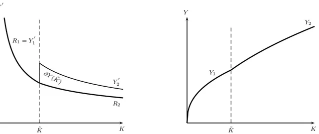
2.5. Global production and return functions
Given that the critical value ˜K defines a switching boundary, the endogenous markup function given by equation (16) has two contiguous branches. Thus, the aggregate production function in (14) and the rate of return on capital in (12) also exhibit two contiguous branches:
Y(K) =
Y1(K)≡(1− 1σ)F(K) if 0≤K ≤K˜,
Y2(K)≡(1−m(K))F(K) ifK ≥K˜,
(18)
and
R(K) =
R1(K)≡(1− 1σ)F
′
(K) if 0≤K ≤K˜,
R2(K)≡(1−m(K))F
′
(K) ifK ≥K˜.
(19)
11
Given that m(K) is positive, monotonous and has limK→0m(K) = +∞, limK→∞m(K) = 0, then ˜
K ≡ {K : m(K) = 1/σ} is unique. Therefore: (1) for allK in the interval (0,K˜) we have m(K)>1/σ
which implies µ = min{m(K),1/σ} = 1/σ, and (2) for all K in the interval in the interval ( ˜K,+∞) we
The first branch in both functions corresponds to the MC regime and the second cor-responds to the CMC regime. Next we will characterize the properties of the aggregate technology and return on capital arising from those functions.
At K = ˜K both production and return functions are continuous, because
R1( ˜K) = R2( ˜K) = ˜R =α(σ−1)(A/σ) ˜Kα−1
Y1( ˜K) = Y2( ˜K) = ˜Y = (σ−1)(A/σ) ˜Kα,
but classic derivatives do not exist. However, we can determine generalized gradients for the production function as
∂Y(K) =
Y′
1(K) if 0 ≤K <K˜, ∂Y( ˜K) ifK = ˜K,
Y′
2(K) if K >K˜.
(20)
where∂Y( ˜K) is the convex hull ofY′
1(K) and Y
′
2(K) atK = ˜K,∂Y( ˜K) ={(1−q)Y
′
1( ˜K) + qY2′( ˜K) : 0 ≤q≤1}, and for the return function
∂R(K) =
R′
1(K) if 0≤K <K˜, ∂R( ˜K) ifK = ˜K,
R′
2(K) ifK >K˜,
(21)
where∂R( ˜K) is the convex hull ofR′
1(K) andR
′
2(K) atK = ˜K,∂R( ˜K) ={(1−q)R
′
1( ˜K) + qR′
2( ˜K) : 0≤q ≤1}.
Lemma 1. FunctionsY(K) and R(K) are continuous and piecewise smooth (PWS).
All proofs are in the appendix. Next we observe that the concavity of both functions depend critically on the elasticity of intermediate input substitution, σ. Let us define
¯
σ= ¯σ(α) = 2−α
2(1−α) >1, (22)
Lemma 2. LetK¯ ≡(¯σ/σ)2/αK˜. (a) If the elasticity of substitution between inputs is large, i.e. for σ > σ¯, then the technology is concave in a generalized way, i.e. ∂2Y(K) ∈ R
−−,
and there are decreasing returns, i.e. ∂R(K) ∈ R−−. (b) If max{1,σ/¯ 2} < σ < σ¯ then
the production function is concave and the return function is non-monotonous: R2(K) is
increasing for K ∈ [ ˜K,K¯), reaches a local maximum at K = ¯K, and it is decreasing for
K > K¯. (c) If 1 < σ < max{1,σ/¯ 2} then the return function has the same properties as in (b) but the production function becomes concave-convex: Y2(K) is locally convex for K ∈[ ˜K,K¯), reaches a local maximum at K = ¯K, and it is locally concave for K >K¯. 12
Figures A.1 and A.2 below depict the first two (more plausible) cases in which the pro-duction function is concave, i.e. forσ >σ¯, and the case in which the return function may be locally increasing, at the onset of the CMC regime, and the production function is concave.
Figure A.1 around here
Figure A.2 around here
The existence of two regimes has interesting economic implications. First, the firm-level production technology is one corresponding to ”natural monopoly” since there is a globally decreasing average cost whenφ >0 with constant marginal cost. The degree of inefficiency can be proxied by the gap between average cost (ac) and marginal cost (mc). In both MC and CMC regimes free entry implies that price equals average cost p=ac (zero profits) and industry equilibrium implies marginal revenue, p(1−1/(nσ)), equals marginal cost: hence
ac mc =
1− 1 nσ
.
In the MC regime where n = 1, this gap is fixed and hence output per-firm is tied down. In the CMC regime, however, matters are different because n increases with K, n =
12
(σφ/F(K))−1/2. More firms means a lower markup, which narrows the gap between ac
and mc, as the zero-profit condition requires output per firm to increase. In the limit as K
(and hence n) tend to infinity, ac tends to mc, and output per firm also tends to infinity, the condition for efficient production.
The possibility of a concave-convex technology relates to an existing literature: Skiba (1978) and Dechert and Nishimura (1983). However, these contributions were made for centralized economies in which the externalities are fully internalized. Therefore, the return and the marginal product of capital are permanently equalized. In our model we retain some of the dynamic properties of that type of model (e.g. the existence of multiple stationary equilibria) while circumventing criticisms that those functions are ad-hoc. In addition, when utility is logarithmic, the general equilibrium is Markovian in contrast to those models - see Santos (2002) (see below).
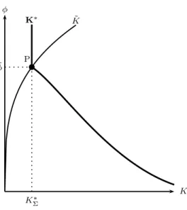
3. General Equilibrium
Definition 1. General Equilibrium The general equilibrium (GE) is defined by the paths
for the mass of industries and for the number firms per industry, [(z(t), n(t))]∞
t=0, by the
allocations and prices[([y(v, t)]v∈(0,z(t)],[p(v, t)]v∈(0,z(t)])]∞t=0, and by the aggregate capital stock
and consumption trajectories [(K(t), C(t))]∞
t=0 such that both final- and intermediate-goods
firms and consumers optimize, there is symmetric equilibria in all markets for intermediate
goods, and the equilibrium conditions for both factor and final-good markets hold.
In the previous section, we proved that in a symmetric equilibrium, the paths of z, n, and of the distributions [y(v)] and [p(v)] depend on the paths of the aggregate capital stock
K, and the last one is jointly determined with the trajectory of aggregate consumption C
at the GE level. AsR(K) andY(K) are defined by the PWS continuous functions (18) and (19) the GE paths are generated by a dynamic system that also displays discontinuities.
Let us define the following subsets of (K, C)∈R2+:
Σ = {(K, C)∈R2+ :m(K) = 1/σ}={ (K, C)∈R2+ :K = ˜K}, (24)
S2 ={ (K, C)∈R2+:m(K)<1/σ}={ (K, C)∈R2+ :K >K˜}, (25)
where S1 (S2) corresponds to states of the economy where a MC (CMC) regime is in place. If the economy is in state Σ we say it is on the switching boundary between the previous two regimes. We also know that ¯S1∩S2¯ = Σ.
The equilibrium trajectories [(K(t), C(t))]t∈R+ are the solutions to the system
˙
C =
(R1(K)−(ρ+δ))C if (K, C)∈ S1,
(R2(K)−(ρ+δ))C if (K, C)∈ S2,
(26)
˙
K =
Y1(K)−δK−C if (K, C)∈ S1,
Y2(K)−δK−C if (K, C)∈ S2.
(27)
together with the initial condition K(0) =K0 and the transversality condition in (3).
Equations (26) and (27) define a PWS continuous dynamic system since: (1) both functions are smooth in the two branches; (2) they are continuous at the boundary Σ, as R1( ˜K) = R2( ˜K) and Y1( ˜K) = Y2( ˜K); and (3) nevertheless, their derivatives differ at K = ˜K, i.e. R′
1( ˜K) < R
′
2( ˜K) and Y
′
1( ˜K)< Y
′
2( ˜K) 13. In order to understand the nature of
the dynamics of our PWS system, we have distinguish betweencandidate and GE paths. We denote them as Φc(t) = (Φc
K(t, K(0)),ΦcC(t, K(0))) and Φ(t) = (ΦK(t, K(0)),ΦC(t, K(0)))
respectively. Candidate trajectories, are solutions to the system (26)-(27) for a given ini-tial capital stock K(0), belonging to one of the two possible states of the economy: MC when 0 < K(0) < K˜ (branch S1) or CMC when K(0) > K˜ (branch S2). We denote
13
Were the functions discontinuous at the boundary Σ, we would have a Filippov system, from Filippov
(1988). See di Bernardo et al. (2008), and Leine and Nijmeier (2004) for the state of the art on the analysis
of both types of dynamic systems. Fillipov systems have been subject to more attention. However, recent
advances in dealing with PWS continuous systems are presented in the above-mentioned references and also
in Freire et al. (1998) and Leine (2006). We will use the approach in di Bernardo et al. (2008) and di
Φc
j(t) = (Φcj,K(t),Φcj,C(t)) and Φj(t) = (Φj,K(t),Φj,C(t)) the candidate and the GE
trajecto-ries belonging to branch Sj forj = 1,2.
The following types of behavior are possible, starting from any initial capital stock14:
if (K(0), C(0)) ∈ Sj for j = 1,2, with an arbitrary C(0), the solution Φc(t) = Φcj(t), for
t > 0, has one the following alternative types of trajectory. First, it may stay inside the same area Sj converging to a steady state (Kj∗, Cj∗) ∈ Sj, or it may converge to zero or
unbounded values for one or both variables. Alternatively, it may contact the boundary Σ at time t = tΣ > 0 where Φcj,K(tΣ, K(0)) = ˜K. It was proved that for PWS continuous
systems15 four types of behavior may unfold upon contact with the switching boundary: (1)
there is a steady state located at the boundary ( ˜K,C˜)∈Σ, which is reached in infinite time and we have Φc
j(∞, K(0)) = (CΣ∗, KΣ∗); (2) the trajectory crosses the boundary and proceeds
to S−j (S−j =S1 forj = 2 andS−j =S2 for j = 1), taking the value Φc−j(t,Φcj(tΣ, K(0)) at
time t > tΣ and converges to a steady state (K−∗j, C−∗j) ∈ S−j to zero or unbounded values
of one or both variables; (3) the trajectory grazes the boundary and turns back inside area
Sj, converging to a steady state (Kj∗, Cj∗)∈ Sj to zero or to unbounded values of one or both
variables; (4) the trajectory crosses Σ at timetjΣ, penetratesS−j, curls back to the switching
boundary Σ at time t−Σj > tjΣ, and re-enters the initial branch Sj - in this case, ift > t−Σj the
candidate path takes the value Φc
j(t,Φc−j(t
−j
Σ ,Φcj(t j
Σ, K(0))).
GE trajectories, Φ(t), are candidate trajectories starting from a given (K(0), C(0)) ∈ Sj
such that the transversality condition holds. If the equilibrium is determinate, there is an unique value Φj,C(0, K(0)) such that the transversality condition holds, whether that
value is not unique when indeterminacy exists. In our case this means that the trajectories should converge to a steady state in Sj (with or without grazing the boundary Σ), in Σ or
in S−j, after traversing the boundary. If the last case occurs, the GE paths concatenate
14
It is well known in the literature that solutions exist when the vector fields are continuous, as in our
model.
15
the solutions belonging to both branches. If (K(0), C(0)) ∈ Sj then Φ(t) = Φj(t, K(0))
for t < tΣ, Φ(tΣ) = Φj(tΣ, K(0)) for t = tΣ, and Φ(t) = Φ−j(t,Φj(tΣ, K(0)), for t > tΣ.
Intuitively, this means that there is an endogenous and transient change in the regime from MC to CMC, or vice-versa.
Thus, two possible changes in regime may occur: (1) a transient change in regime takes place if the initial and the steady-state levels for the capital stock are located in different sides of the switching boundary Σ and the adjustment dynamics involves traversing the switching boundary; (2) a long-run regime shift occurs if there is a parameter change that justifies it.
In the next two sections, we use global-bifurcation analysis to determine what types of GE dynamics features our model can display. We do this by characterizing the local behavior at equilibria, the behavior at the switching boundary, and finally global dynamics.
4. Local Dynamics
We will first examine local dynamics around the steady-states. In the last section we presented two types of steady states that can exist in system (26)-(27): regular steady states
if they belong to the interior of Sj with j = 1,2, (Kj∗, Cj∗) ≡ {(K, C)∈ Sj : ˙C = ˙K = 0},
and boundary steady states if they belong to Σ, (K∗
Σ, CΣ∗)≡ {(K, C)∈Σ : ˙C = ˙K = 0}. For
given values of the parameters, steady states may be isolated or multiple, and in the latter they can belong either to the same or to different regimes.
From the properties of functions (18) and (19) we obtain the following relationship be-tween steady-state consumption and capital stock:
C∗
j =βKj∗, β ≡
ρ+ (1−α)δ
α >0,forj = 1,2,Σ, (28)
which implies that each steady state is completely characterized using the steady-state stock of capital,K∗
Let us define the following critical values for parameter φ:
˜
φ≡ 1 σ
A
α ρ+δ
1− 1 σ
α1/(1−α)
. (29)
and
¯
φ≡ σ
¯
σ2
A
α ρ+δ
1− 1
¯
σ
α1/(1−α)
for 1< σ ≤σ¯. (30)
The next proposition and the bifurcation diagrams in Figure A.3 summarize the local dynamics, in the neighborhood of steady states.
Proposition 1. Local dynamics and bifurcations at steady-state equilibria.
1. If1< σ <σ¯either a unique or multiple equilibria may exist, depending onφ. Forφ >φ¯
there is a unique saddle-point stable regular MC equilibrium. For φ < σ <˜ σ¯ there are three regular equilibria, a MC saddle-point stable and a pair of CMC equilibria: a
high-markup unstable and a low-high-markup saddle-point stable. For φ < φ˜ there is a unique saddle-point stable CMC equilibrium. For φ= ¯φ there are two steady states: a saddle-point stable regular MC and a regular CMC that is locally a smooth-fold bifurcation. For
φ= ˜φ there are two equilibria: a saddle-point stable CMC equilibrium and a boundary equilibrium displaying a non-smooth fold bifurcation.
2. If σ ≥ σ¯ there is a unique equilibrium whose type depends on φ. For φ > φ˜ it is a saddle-point stable MC equilibrium. For φ < φ˜ it is a saddle-point stable CMC equilibrium. Forφ = ˜φ it is a boundary-equilibrium bifurcation displaying saddle-point stable persistence.
We will derive Proposition 1 step by step in the next sub-section 4.1. However, first we will interpret its meaning and implications.
Figure A.3 around here
different values of the fixed cost it shows the number of equilibria and the local stability prop-erties of each steady-state equilibrium, including the location of the discontinuity-induced bifurcations (persistence P on the RHS panel and the non-smooth fold NF on the LHS panel) and the smooth fold bifurcation (F on the LHS panel).
If we start with high values ofφ, on the RHS panel, the initial equilibrium is saddle-point stable (C∗
M, KM∗ ), it is a MC equilibrium, and further reductions of the fixed cost keep the
local stability properties, but force it to pass through the switching boundary (C∗
Σ, KΣ∗) and
further evolve into a CMC equilibrium (C∗
L, KL∗). We associate the later to a low markup as
the return function is locally decreasing.
If we do the same reasoning for the left-hand-panel panel, we should observe that there is structural instability, i.e. there is a change on the number of equilibria and on their local-dynamics properties for variations of φ close to its bifurcation levels: ˜φ associated to a discontinuity-induced bifurcation of the non-smooth fold type16, and ¯φ associated to a
smooth fold bifurcation. If we start with high values of φ the initial equilibrium (C∗
M, KM∗ )
is also saddle-point stable and it is a MC equilibrium. If we reduce φ from ¯φ, then three equilibria emerge: (C∗
M, KM∗ ), an unstable high-markup CMC equilibrium (CH∗, KH∗), and a
saddle-point stable low-markup equilibrium (C∗
L, KL∗). Further reductions ofφfrom ˜φ, would
result in the collision of the first two equilibria at the discontinuous boundary equilibrium bifurcation point (C∗
Σ, KΣ∗), followed by their disappearance. For lower values ofφthe
steady-state equilibrium is unique and again it is a saddle-point stable low-markup CMC (C∗
L, KL∗).
Observe that the MC steady-state level for the capital stock does not depend on φ. However, when the fixed cost varies, the distance to the switching boundary changes: if the fixed cost increases, the ”competitive distance” increases. If the economy is in the CMC regime, not only the distance of the steady state to the switching boundary varies (because
˜
K depends on φ), but the steady-state stock of capital also varies. If the elasticity σ is low and there are multiple CMC equilibria the relative ”competitive distance” of the two
16
equilibria changes in a symmetric way. When the fixed cost is reduced, the unstable high-markup equilibrium moves towards the switching barrier and the low-high-markup saddle-point stable equilibrium moves away from it.
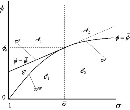
We can also observe the same by defining a partition over the domain of (φ, σ), i.e.
R++×(1,+∞) - see Figure A.4:
A={ (σ, φ) :σ >1, φ >max{φ,φ˜}}, DF ={ (σ, φ) : 1< σ <σ, φ¯ =φ},
B={ (σ, φ) : 1< σ <σ,¯ φ < φ < φ˜ }, DN F ={(σ, φ) : 1 < σ <¯σ, φ= ˜φ},
C ={ (σ, φ) :σ >1, 0< φ <φ˜}, DP ={ (σ, φ) :σ > 1, φ = ˜φ}.
Figure A.4 around here
This pair of crucial parameters allow us to identify the region where steady-state equi-libria lie. If (σ, φ)∈ A, given by A1∪ A2 in Figure A.4 , there is a single saddle-point stable stationary MC equilibrium (K∗
M, CM∗ ) ∈ S1. If (σ, φ) ∈ C, given by C1 ∪ C2 in the same
picture, there is a unique saddle-point stable stationary CMC equilibrium (K∗
L, CL∗) ∈ S2.
If (σ, φ)∈ B, three stationary equilibria exist: the saddle-point stable stationary MC equi-librium (K∗
M, CM∗ ) ∈ S1 and the two CMC equilibria in the S2 region, the saddle-point
stable (K∗
M, CM∗ ) and the unstable (KL∗, CL∗). When we observe the limits between two of
the previous regions bifurcations occur. If (σ, φ)∈ DF ∪ DN F two stationary equilibria exist
with a fold bifurcation associated to one of them: on the DF frontier the bifurcation is a
regular smooth one and on the DN F border it is a non-smooth one. Finally, if (σ, φ) ∈ DP
persistence is the discontinuity-induced bifurcation that emerges. We can find a single saddle-point stable MC equilibrium like (K∗
M, CM∗ ) in dynamic GE
models with a Dixit and Stiglitz (1977) MC market structure - see Rotemberg and Woodford (1995). Gal´ı and Zilibotti (1995) present a CMC model that produces a pair of equilibria that correspond to (K∗
L, CL∗) and (KH∗, CH∗), with the possibility of complex eigenvalues for
existence of endogenous markups is not a sufficient condition to generate multiple equilibria as we can see in Goodfriend and King (1997), Jaimovich (2007) or even in the CMC model of Portier (1995).
4.1. Derivation of 1
Our first step is to establish the existence and number of steady states:
Lemma 3. Let σ¯, φ,˜ and φ¯ be given by equations (22), (29), and (30), respectively. Then: (1) if φ > max{φ,˜ φ¯}, for any σ > 1, there is a unique regular MC steady state; (2) if
0< φ <min{φ,˜ φ¯}, for any σ > 1, there is a unique regular CMC steady state; (3) if σ≥σ¯
and φ = ˜φ then there is a unique boundary steady state; (4) if 1< σ < σ¯ and φ < φ <˜ φ¯, there are three regular steady states, a MC and two CMC steady states; (5) if1< σ <σ¯ and
φ = ¯φ, there are two regular steady states, one MC and the other CMC; (6) if 1 < σ < σ˜
and φ = ˜φ, there are two steady states, a regular CMC and a boundary one.
If the elasticity of substitution between varieties is large, σ≥σ¯, then the steady state is unique, but it may be associated to any regime or belong to the switching boundary. The type of steady-state regime depends on the cost of entry φ relative to the other parameters. First, if the fixed cost is high (or A is low) such that φ > φ˜then there is a unique regular MC steady state that we can determine explicitly
K∗
1 =KM∗ ≡
αA ρ+δ
1− 1 σ
1/(1−α) <K˜.
Second, if the fixed cost is low (or A is high), such that φ < φ˜, then there is a regular CMC steady state which is unique from Lemma 3, with capital stock defined by
K∗
2 ={ KC∗} ={K ∈ S2 : (1−m(K))F
′
(K) =ρ+δ}.
In the transition between those two cases, i.e. if φ = ˜φ, then the steady-state capital stock is given by
KΣ∗ = ˜K( ˜φ) = σφ˜
αA !1/α
=
α2A ρ+δ
1− 1 σ
1/(1−α)
If the elasticity is low, verifying 1 < σ < σ¯ several cases may occur. In this case we have ˜φ < φ¯ and both similar and different possibilities are produced, as in the case of high σ. If φ > φ¯ or φ < φ˜ we have two cases that are analogous to the previous high-elasticity ones: we observe unique steady states associated with either K∗
M orKC∗. However,
if ¯φ > φ >φ˜multiple steady states exist: a regular MC, K∗
M, and two regular CMC steady
states, K∗
2 ={KH∗, KL∗} such that
˜
K∗
Σ < KH∗ <K¯∗ < KL∗,
where
¯
K∗ = ¯K( ¯φ) =
αA ρ+δ
1− 1
¯
σ
1/(1−α)
.
As m(K∗
H) > m(KL∗), we call them high- and low-markup CMC steady states,
respec-tively. At last, in the boundary cases, associated to either φ = ¯φ or φ = ˜φ, there are two steady states. In the first case there is regular MC, K∗
1 = KM∗ , and a CMC steady state,
K∗
2 = ¯K∗, and, in the second case, there is a boundary,KΣ∗, and a regular low-markup CMC
steady state, K∗
2 =KL∗. As we will see below, both cases are associated to local bifurcations,
a smooth or classic one, in the first case, and a non-smooth, in the second. The steady state ¯
K∗ occurs at the local maximum of the R
2(K) function if the return function is globally
non-decreasing.
In order to study the local stability and bifurcation properties, we build the generalized Jacobian in the sense of Clarke (see Clarke (1990) and Leine (2006))
J(K∗) =
J1(K1∗), if (K1∗, C1∗)∈ S1,
J(K∗
Σ), if (KΣ∗, CΣ∗)∈Σ, J2(K2∗), if (K2∗, C2∗)∈ S2.
If we have a regular steady state belonging to the interior of subset Sj, j = 1,2 the classic
Jacobian is
Jj(Kj∗) =
0 Cj(Kj∗)R
′
j(Kj∗)
−1 Cj′(Kj∗)
where Cj(Kj∗) ≡ Yj(Kj∗)−δKj∗ for Kj∗, Cj∗
∈ Sj, j = 1,2. If we have a boundary steady
state, K∗
Σ = ˜K, the classic Jacobian does not exist, but we can determine the generalized
differential of Clarke evaluated at that point as the convex hull of the derivatives at that point, which in our case becomes
J(K∗
Σ) ={(1−q)J1(K) +qJ2(K) : 0≤q≤1, K =KΣ∗},
as the boundary steady state is completely characterized by the capital stock level K∗ Σ.
The eigenvalues of the Jacobians associated to regular steady states are
λ−
j = Cj′(Kj∗)
2 −∆(Jj(K ∗
j))1/2, λ+j = Cj′(Kj∗)
2 + ∆(Jj(K ∗
j))1/2, for j = 1,2,
where the discriminant is
∆(Jj) =
Cj′(Kj∗)
2
!2
−Cj(Kj∗)R
′
j(Kj∗),j = 1,2.
The eigenvalues are continuous functions of the parameters, in particular of φ and σ. If, as a result of a continuous change in a parameter, at least one eigenvalue associated to a regular steady state crosses the imaginary axis we say the equilibrium point (K∗, C∗)
undergoes a smooth bifurcation17.
Lemma 4. 1. Assume there is a regular MC steady state (K∗
1, C1∗) ∈ S1. Then it is
saddle-point stable.
2. Assume there is a regular CMC steady state (K∗
2, C2∗) ∈ S2. Then, if R
′
2(K2∗) < 0
it is saddle-point stable, if R′
2(K2∗) > 0 it is a non-oscilatory unstable node, and if R′2(K∗
2) = 0 it is a smooth fold bifurcation point.
17
For the existence of classic or smooth bifurcations in PWS dynamic systems see di Bernardo et al. (2008).
Local dynamics and bifurcations in the neighborhood of boundary steady states for PWS continuous systems have been studied in the applied mathematics literature, though there are different approaches and nomenclatures18. di Bernardo et al. (2008) use the
expres-sion discontinuity-induced bifurcations for a generic change in structural stability in a PWS dynamic system, upon a change in a parameter. There is a boundary-equilibrium bifur-cation at a boundary steady state, K∗
Σ, if for φ = ˜φ the Jacobians at the boundaries of
the two contiguous branches, S1 and S2, verify det (Jj(KΣ∗,φ˜)) 6= 0, for j = 1,2. Two
types of boundary-equilibrium bifurcations may exist: persistence, if at the bifurcation point (K∗
Σ, CΣ∗) a regular equilibrium in branch Sj is turned into a regular equilibrium in branch
S−j after a small variation in the bifurcating parameter, φ; or non-smooth fold, if there is a
collision on the boundary of two regular steady states with different stability properties from both branches, and we observe their disappearance after a small change in the bifurcating parameter.
Lemma 5. Let (K∗
Σ, CΣ∗) be a boundary steady state. Then a boundary-equilibrium
bifurca-tion occurs at φ = ˜φ if σ 6= ¯σ19. If 1< σ <σ¯, there is a non-smooth fold bifurcation and if σ >σ¯, there is persistence.
We need to determine the eigenvalues of the Jacobian in order to have a specific char-acterization of the local dynamics at the boundary steady state. As the Jacobian J(K∗
Σ) is
set-valued, so are its generalized eigenvalues,
Λ±(KΣ∗) =
λ±Σ(q) : 0≤q ≤1 ,
where λ±Σ(q) are the eigenvalues of the generalized Jacobian JΣ(q) ≡ J(KΣ∗, q) = (1 − q)J1(KΣ∗) +qJ2(KΣ∗). Observe that, although λ±Σ(0) = λ
±
1(KΣ∗) and λ±Σ(1) = λ ±
2(KΣ∗), we
18
For two alternative approaches see Leine and Nijmeier (2004) or di Bernardo et al. (2008). On
local-bifurcation analysis see Freire et al. (1998), Leine (2006), and the previous references.
19
This is a co-dimension-one bifurcation. Ifφ= ˜φandσ= ¯σa co-dimension-two type of bifurcation may
have λ±
Σ(q)6= (1−q)λ ±
1(KΣ∗) +qλ±2(KΣ∗).
Lemma 6. The generalized eigenvalues Λ±(K∗
Σ) are real. If σ > σ¯ then Λ− ⊂ R−− and
Λ+ ⊂ R
++. If 1 < σ < σ¯ then Λ− ⊂R and Λ+ ⊂ R++. In this case there is a value for q, q0 ≡(σ−1)/(¯σ−1) such that λ−Σ(q0)) = 0.
If we consider Lemmas 5 and 6 together we can conclude the following. If the elasticityσis large and the bifurcation parameterφis reduced continuously towards ˜φ, in the neighborhood of a boundary steady state, a saddle-point regular MC steady state is continued as a saddle point at the boundary-equilibrium bifurcation, and for further reductions, into a saddle-point regular CMC steady state. This is the meaning of persistence in our case. On the other hand, if the elasticity σ is low and φ is slightly larger than ˜φ there will be two regular steady states, a saddle-point stable MC and an unstable CMC, which, upon reduction of the fixed cost will both collide at the boundary steady state and will both disappear for further reductions. This is the particular instance of a non-smooth fold bifurcation in our model. This type of behavior is generated by a discontinuity in the first derivatives which does not occur in smooth dynamic systems.
4.2. Local dynamics at the switching boundary
Candidate trajectories, including equilibrium trajectories presented in section 3, may contact the switching boundary in infinite time when there is a boundary steady-state equi-librium. If σ > σ¯, equilibrium trajectories converge to it along the saddle paths passing through (K∗
Σ, CΣ∗). Piecewise smoothness of the vector field implies that the slopes of the
saddle paths are not collinear in both branches separated by Σ. If σ <σ¯ equilibrium trajec-tories converge to the boundary equilibrium ifK(0)< K∗
Σ and they diverge from it, moving
towards the low-markup CMC equilibrium if K(0) > K∗
Σ. This is the consequence of the
existence of a non-smooth fold bifurcation.
in the study of this behavior use the Filippov convex method, as we do below (see Filippov (1988), and Leine and Nijmeier (2004)).
Let us write compactly the vector fields in the two sub-domains asfj(K, C) for (K, C)∈
Sj and j = 1,2. Accordingly we will use the vector-field notation ˙C = fj,C(K, C), i.e. the
RHS of equation (26), and ˙K =fj,K(K, C), i.e. the RHS of equation (27), again for (K, C)∈
Sj with j = 1,2. Consider a trajectory that reaches the switching boundary Σ at time tΣ,
Φc
j(tΣ) ∈ Σ, coming from branch Sj ( j = 1,2). Recalling the definition of Σ in equation
(24), we know that Φc
j,K(tΣ) = ˜K. Let us define the function h(K, C)≡m(K)−1/σ. The
behavior of the vector field fj(·), as regards the normal to Σ, can be obtained from the
following two functions vj(K, C) and aj(K, C):
vj(K, C) =
∂ ∂th Φ
c j(0)
=Lfjh(K, C), j = 1,2, (32)
and
aj(K, C) =
∂2 ∂t2h Φ
c j(0)
=L2fjh(K, C), j = 1,2, (33)
where Lfjh and L
2
fjh are the first and second Lie derivatives of function h(K, C) evaluated
at (K, C)∈Σ, along the projections of vector fieldfj(·) into the normal of h(K, C) = 0:
Lfjh(K, C) =
∂h ∂Cfj,C+
∂h
∂Kfj,K, (34)
and
L2fjh(K, C) = ∂
∂C
∂h ∂Cfj,C+
∂h ∂Kfj,K
fj,C+
∂ ∂K
∂h ∂Cfj,C+
∂h ∂Kfj,K
fj,K. (35)
The literature on PWS continuous systems tells us that there are two main types of con-tact of trajectories originated in branch Sj with the switching boundary, when no boundary
equilibrium points exist: traversing or grazing trajectories. This allows a partition of the switching boundary into a traverse subset,
and a subset in which grazing is observed inside Sj
Σgj ≡ { (K, C)∈Σ :vj(K, C) = 0, aj(K, C)6= 0}.
The full grazing subset is defined as Σg = Σg
1 ∪Σ
g
2.
Given our definitions of sets Sj in equations (23) and (25), and the fact that h(K, C)>0
(h(K, C) < 0) for K < K˜ (K > K˜), if Lfjh(K, C) > 0 the trajectory crosses Σ in the
direction of a decreasing K and if Lfjh(K, C) < 0 it crosses the boundary in the direction
of an increasing K. Also, if a grazing point exists, the structure of h(·) implies that, for
aj(K, C)>0, grazing takes place from side S1.
Lemma 7. Let C˜ =Y1( ˜K)−δK˜ =Y2( ˜K)−δK˜. Then:
1. Σt={( ˜K, C) :C 6= ˜C};
2. For any values of the parameters, ifΦc
C( ˜K, tΣ)>C˜ then candidate trajectories traverse
Σ by decreasing K, i.e. ∂Φc
j,K( ˜K, tΣ)/∂t < 0, for j = 1,2. If ΦcC( ˜K, tΣ) < C˜ then
candidate trajectories traverse Σ by increasing K, i.e. ∂Φc
j,K( ˜K, tΣ)/∂t > 0, for j =
1,2.
3. Ifφ <φ˜thenΣg = Σg
1 ={( ˜K,C˜)}andΣ
g
2 is empty. Ifφ >φ˜thenΣg = Σ
g
2 ={( ˜K,C˜)}
and Σg1 is empty.
From Lemma 7 we conclude that grazing is unilateral. For φ < φ˜, there is a candidate trajectory which grazes Σ within S1, i.e. Φc
1,C( ˜K, tΣ) = ˜C. Forφ > φ˜, there is a candidate
trajectory which grazes Σ within S2, i.e. Φc
2,C( ˜K, tΣ) = ˜C. di Bernardo et al. (2008) call a
point like ( ˜K,C˜) aregular grazing point.
We call grazing trajectory to a candidate trajectory that is tangent to Σ. If grazing happens to trajectories insideSj, then a grazing trajectory separatesSj into a subset in which
trajectories departing from inside of it approach Σ, but do not collide with the boundary and curl back intoSj, from a subset in which trajectories starting within traverse the boundary Σ
two types of behavior: either they curl back to Σ and traverse it returning to Sj, or they
continue only at branchS−j. Then there is a separating trajectory, that tends to converge to
an equilibrium point in Sj. In fact, this trajectory is the GE trajectory and belongs to the
stable manifold associated to a stationary equilibrium point. From this, we conclude that grazing trajectories are candidate trajectories but are not GE trajectories.
5. Global General-Equilibrium Dynamics
Apparently, explicit solutions for equilibrium (and candidate) trajectories do not exist, so we have to resort to qualitative analysis of the equilibrium dynamics by drawing on the results from the two previous sections.
There are two main results in terms of global GE dynamics. First, there is the possibility of transient or long-run change in regime from MC to CMC, depending on the relationship between the fixed cost and the initial level of the capital stock to the remaining parameters in the model. Second, there is the dependence of the structural dynamics on the curvature properties of the return function, which is related to the elasticity of substitution amongst varieties.
Next we present the most representative GE trajectories using phase diagrams for the cases where there is either a unique steady-state equilibrium or multiple long-run equilibria.
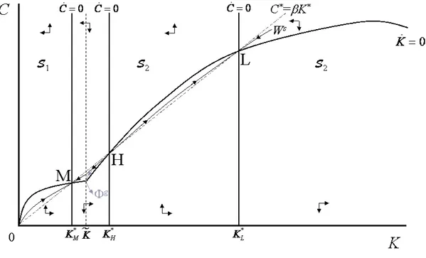
Proposition 2. Let φ > max{φ,¯ φ˜}, for any σ > 1, and assume that K(0) > 0. Then there is a unique saddle-point stable MC stationary equilibrium (K∗
M, CM∗ ). The GE path
[Φ(t, K(0))]t≥0, where Φ(t) = (ΦK(t),ΦC(t))⊤, converges asymptotically to (KM∗ , CM∗ ),
inde-pendently of the regime associated to K(0) at time t = 0. In particular, if K(0) > K˜ then both capital and consumption adjust downwards, the convergence is PWS continuous, the
equilibrium path verifies ΦK(tΣ, K(0)) = ˜K, where tΣ > 0 is the time of collision with the
boundary Σ, and ΦgC(t, K(0)) < ΦC(t, K(0)) < βΦK(t, K(0)) for 0 < t ≤ tΣ, where [Φg(t)]
Figure A.5 depicts the complete phase diagram associated to Proposition 2. If the initial capital stock satisfies 0 < K(0) < K˜ then both the initial and the stationary state of the economy exhibit a MC regime and the markup is constant, i.e. it is independent of the transitional dynamics. The dynamics is smooth in this region (S1) and it depends on the relative position of K(0) regarding K∗
M. If K(0) is greater (smaller) than KM∗ , then
there is a downward (upward) adjustment in both variables. If the initial capital stock is above the switching boundary, i.e. if K(0) > K˜, then the economy starts from a CMC regime and it shifts to the MC regime along the transition path at time t = tΣ. In the
beginning of the adjustment the markup is endogenous and counter-cyclical: both output and consumption decrease while the markup adjusts upwards. At time tΣ there is exactly
one firm per industry, as the economy switches from a CMC to a MC regime. At this point, the markup becomes exogenous and constant while the mass of the continuum of varieties shrinks continuously along the convergence to the stationary equilibrium (K∗
M, CM∗ ). The GE
equilibrium path lies along the stable manifold associated with MC equilibrium, represented by Ws
M = Ws(KM∗ , CM∗ ), which belongs to both branches S1 and S2, and is therefore
non-smooth. Notice that for K(0)> K∗
M the stable manifold lies between the schedule C =βK
and the PWS isocline ˙K = 0.
Figure A.5 around here
Proposition 3. Let φ < min{φ,¯ φ˜}, for any σ > 1, and assume that K(0) > 0 . Then there is a unique saddle-point stable CMC stationary equilibrium (K∗
L, CL∗). The GE path
[Φ(t, K(0))]t≥0, whereΦ(t)converges asymptotically to (KL∗, CL∗), independently of the regime
associated to K(0) at time t = 0. In particular, if K(0) < K˜ then both capital and con-sumption adjust upwards, the convergence is PWS continuous, the equilibrium path
veri-fies ΦK(tΣ, K(0)) = ˜K, where tΣ > 0 is the time of collision with the boundary Σ, and
ΦgC(t, K(0)) > ΦC(t, K(0)) > βΦK(t, K(0)) for 0 < t ≤ tΣ, where [Φg(t)] is the grazing
Figure A.6 depicts the complete phase diagram associated to Proposition 3. The inter-pretation is similar to that of Figure A.5. The GE equilibrium path lies along the stable manifold associated with the low-markup CMC equilibrium, Ws
L =Ws(KL∗, CL∗), which also
belongs to both branches S1 and S2, and is non-smooth. In this case, if the initial state of the economy is in the MC regime and the initial capital stock lies in the interval 0,K˜, then it increases in the transition and there is a switch in the regime along the way. In the beginning, the markup is uncorrelated with economic activity, but then intra-industrial entry occurs as soon as the capital stock reaches ˜K. From that point onwards competition will drive the markup counter-cyclically down.
Figure A.6 around here
Multiple steady-state equilibria exist in the remaining cases. Here we deal with the generic case in which 1 < σ < σ¯ and ˜φ < φ < φ¯. From Proposition 1, we already know that there are three steady-state equilibria, (K∗
M, CM∗ ), (KH∗, CH∗), and (KL∗, CL∗), which are
collinear, i.e. C∗
j =βKj∗, j =M, H, L, with KM∗ < KH∗ < KL∗.
As we will show next, two heteroclinic orbits exist. First, there is a smooth hetero-clinic orbit joining the two CMC stationary equilibria (K∗
H, CH∗) and (KL∗, CL∗) denoted by
ΓHL. This heteroclinic orbit lives in subset S2 and coincides with the intersection between
the unstable manifold associated to (K∗
H, CH∗), WHu, and the stable manifold associated to
(K∗
L, CL∗), WLs, i.e. ΓHL =WHu ∩WLs. There is also a second, PWS heteroclinic orbit, ΓHM,
joining the CMC equilibrium (K∗
H, CH∗)∈ S2 to the MC equilibrium (KM∗ , CM∗ )∈ S1. Again,
the heteroclinic orbit is defined as the intersection between the unstable manifold associ-ated to (K∗
H, CH∗), WHu, and the stable manifold associated to (KM∗ , CM∗ ), WMs . Therefore,
ΓHM = WHu ∩WMs is continuous, but PWS since it has a discontinuity in its derivatives at
Σ.
Proposition 4. Assume that 1 < σ < σ¯ and φ < φ <˜ φ¯, and also that K(0) > 0. Then there are three stationary equilibria: a MC saddle-point stable equilibrium, (K∗
high-markup CMC unstable equilibrium, (K∗
H, CH∗), and a low-markup saddle-point stable
CMC equilibrium, (K∗
L, CL∗), such that KL∗ > KH∗ > KM∗ and Cj∗ =βKj∗, with j =L, H, M.
If K(0) > K∗
L then the equilibrium path [Φ(t, K(0)]t≥0 adjusts downwards towards the
low-markup equilibrium (K∗
L, CL∗). If K(0) < KM∗ then the equilibrium path converges upwards
to the MC equilibrium (K∗
M, CM∗ ). If KH∗ < K(0) < KL∗ then the equilibrium path converges
upwards to (K∗
L, CL∗) along the smooth heteroclinic trajectory ΓHL. If KM∗ < K(0) < KH∗
then the economy converges downwards to (K∗
M, CM∗ ) along the PWS heteroclinic trajectory
ΓHM.
Figure A.7 around here
Figure A.7 illustrates Proposition 4. The equilibrium trajectory belongs to the stable manifolds associated to (K∗
M, CM∗ ) and (KL∗, CL∗), WMs and WLs. Both these manifolds are
obtained as the union of two branches and exhibit a common point at the unstable steady-state equilibrium (K∗
H, CH∗). The branches that start in this long-run equilibrium feature
heteroclinic trajectories ΓHM and ΓHL. The necessity of the existence of heteroclinic orbits,
which have a global nature, is obvious: the basins of attraction of the two saddle-point stable equilibria should be bounded.
Equilibrium paths are ”trapped” by the two manifolds defined by curves C = βK and
C =C(K), i.e. the isocline ˙K = 0. Geometrically, if the latter is above (below) the former then both capital and consumption increase (decrease).
Depending on the initial level of the capital stock, rational agents ”choose” a MC equilib-rium (K∗
M, CM∗ ) or a CMC equilibrium with a low markup (KL∗, CL∗). The dividing barrier is
given by the CMC equilibrium with a high markup (K∗
H, CH∗). Off course, the economy may
stationary equilibria if the economy is located in one of the sides of the barrier. Nonetheless, there is an important difference: there are restrictions on the possibility of regime shifts along transition paths. If the economy starts from a MC equilibrium it never converges to a CMC stationary equilibrium. However, the converse is not true: if the initial stock of capital associated with a CMC dynamics is such that ˜K < K(0)< K∗
H then the economy converges
to a MC equilibrium. This asymmetry is related to the fact that in this case there is a small elasticity of substitution in the demand for intermediate goods, which can be interpreted as a case where there is an overall low level of flexibility in the economy.
In all the cases in Propositions 2, 3, and 4 the equilibrium is determinate, and it is Markovian (in the sense of Santos (2002)), even for the cases where the function is non-monotonic, similarly to Skiba (1978) and Dechert and Nishimura (1983). However, to our knowledge, this type of global dynamics arising from the change in regime associated to PWS dynamics, has not been analyzed in the macroeconomics literature. The regime switch along the path, linked to the non-smooth dynamics, offers a novel vision on the interaction between the industrial structure of economies and their macroeconomic equilibrium. Reasonably competitive economies may end up in a bad equilibrium if the fixed costs faced by its firms are high. Conversely, economies showing a poor competitive performance may end up in a good (second-best) equilibrium if increasing returns are not substantial.
6. Technology and regime switching
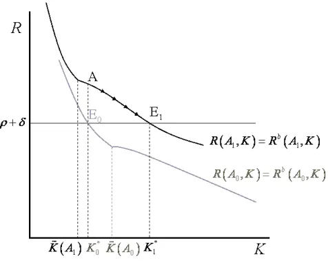
One interesting possibility in this model is the effect of a permanent technological shock, i.e. a permanent increase in A, on the long-run regime of the model. Let us start with the simplest case and assume (σ, φ)∈ A2. The initial long-run equilibrium is depicted by point E0 in Figure A.8. Now, assume there is a permanent technology shock that sets a new value A = A1 > A0. Considering equation (17), then we know that the value for ˜K decreases to
˜
K(A1).
Assume also that K∗
switch from a MC to a CMC regime. Since we know that, for the CMC region, we have
R(K) = (1−m(K))F′(K), an increase inAwill lead to a upward shift in theR(·) schedule,
as ∂m/∂A < 0 and ∂F′/∂A > 0. Following the shock, the economy moves to point A and
eventually to a new long-run equilibrium like point E1 in Figure A.8 20.
Figure A.8 around here
Thus, we can conclude that a small permanent technology shock hitting an economy in a unique stable MC equilibrium close to the switching boundary may have substantial long-run effects since the economy shifts to a CMC regime with a lower equilibrium markup. Of course a negative shock can have the opposite effect. Notice this means the economy is no longer in region A2, as it moved toC2.
The situation is even more interesting when (σ, φ) ∈ B and we have three equilibria. With a similar shock we may have the case depicted in Figure A.9.
Figure A.9 around here
In this case the economy crosses the bifurcation to the A1 region and the new short-run
equilibrium would be given by point A. Considering a permanent shock, there would be new low-markup CMC equilibrium for the long run given by point EP.
Interestingly, even if the shock is temporary, the economy may not go back to E0. Assume
the shock vanishes at t=τ >0, when the economy is at point B. As long as it accumulated enough capital in order to have K(τ) > K∗
H then it jumps to point C at time τ and it
converges to the new steady state E1.
20
The increase in the value ofK∗
In the three-equilibria case, starting from the unstable equilibrium, any shock - no matter how small or temporary - will be sufficient to move the economy towards one of the two stable equilibria. Thus, even temporary shocks can have permanent effects in this economy with multiple equilibria.
7. Conclusion
to the low-output monopolistic equilibrium and with high levels leading to the high-output oligopolistic equilibrium.
In this paper we have assumed that there is an exogenous labor supply: we leave it to further work to see how the dynamics become even richer with an endogenous labor supply. We would also like to relax the assumption of instantaneous free entry, allowing for the flow of entry to be determined by an endogenous cost of entry as in Brito and Dixon (2009): there will be two state variables (the number of firms and the capital stock) driving the markup. This would not affect the steady-state equilibria (since in steady state the cost of entry is zero), but would influence the dynamics out of steady state.
References
Bilbiie, F., Ghironi, F., Melitz, M., 2007. Endogenous entry, product variety, and business cycles. NBER Working Paper 13646.
Brito, P., Dixon, H., 2009. Entry and the accumulation of capital: A two state-variable extension of the ramsey model. International Journal of Economic Theory 5, 333–357.
Chatterjee, S., Cooper, R., Ravikumar, B., 1993. Strategic complementarity in business formation: Aggregate fluctuations and sunspot equilibria. Review of Economic Studies 60, 795–811.
Clarke, F., 1990. Optimization and Nonsmooth Analysis. Wiley, New York.
Costa, L., 2001. Can fiscal policy improve welfare in a small dependent economy with feed-back effects? Manchester School 69, 418–439.
Costa, L., 2004. Endogenous markups and fiscal policy. Manchester School 72 Supplement, 55–71.
D’Aspremont, C., dos Santos Ferreira, R., Grard-Varet, L.-A., 1989. Unemployment in a cournot oligopoly model with ford effects. Recherches Economiques de Louvain 55, 33–60.
D’Aspremont, C., dos Santos Ferreira, R., Grard-Varet, L.-A., 1995. Market power, coordi-nation failures and endogenous fluctuations. In: Dixon, H., Rankin, N. (Eds.), The New Macroeconomics. Cambridge University Press, Cambridge, pp. 94–138.
D’Aspremont, C., dos Santos Ferreira, R., Grard-Varet, L.-A., 1997. General equilibrium concepts under imperfect competition: A cournotian approach. Journal of Economic The-ory 73, 199–230.
Dechert, W., Nishimura, K., 1983. A complete characterization of optimal growth paths in an aggregate model with a non-concave production function. Journal of Economic Theory 31, 322–354.
di Bernardo, M., Budd, C., Champneys, A., Kowalczyk, P., 2008. Piecewise-Smooth Dynam-ical Systems: Theory and applications. Vol. Vol. 163 of Applied MathematDynam-ical Sciences. Springer-Verlag, London.
di Bernardo, M., Budd, C. J., Champneys, A. R., Kowalczyk, P., Nordmark, A. B., Tost, G. O., Piiroinen, P. T., 2008. Bifurcations in nonsmooth dynamical systems. SIAM Review 50 (4), 629–701.
Dixit, A., Stiglitz, J., 1977. Monopolistic competition and optimum product diversity. Amer-ican Economic Review 67, 297–308.
dos Santos Ferreira, R., Dufourt, F., 2006. Free entry and business cycles under the influence of animal spirits. Journal of Monetary Economics 53, 311–328.