UNIVERSIDADE DA BEIRA INTERIOR
Ciências Sociais e Humanas
Do Large Governments Decrease Happiness?
Evidence from European Countries
Tiago Alexandre Silva Minas
Dissertação para obtenção do Grau de Mestre em
Economia
Agradecimentos
Como é óbvio e perfeitamente compreensível, uma dissertação, para além da árdua tarefa científica que representa, consiste igualmente num assertivo e frutífero trabalho de cooperação, onde cada minucioso pormenor e contributo, se resumem no sucesso do resultado final.
Desse modo, tenho a agradecer:
Desde logo, ao Professor Doutor Tiago Sequeira, por me ter aceitado como seu orientando, pela paciência, valiosos contributos, perseverança e apoio incondicional.
Pela motivação e apoio permanente, à minha mais que tudo, àquela a quem mais amo: Rita Almeida.
Pela génese intrínseca de suporte, carinho e amor: à minha mãe e a meu irmão, meus avós e familiares diretos.
A todos os demais, que sempre me apoiaram e acreditaram em mim.
Por que: “O segredo da Felicidade, é encontrar a nossa alegria na alegria dos outros” (Alexandre Herculano)
Resumo
Existem poucas evidências da influência de amplos Governos na Felicidade e, quando existem, são positivas. No presente trabalho mostramos que os Gastos Governamentais Estruturais, assim como outras medidas representativas dos desequilíbrios governamentais, diminuem significativamente a Felicidade e a Satisfação de Vida nos países europeus. Estas evidências devem ser tomadas em linha de conta e conduzir os políticos europeus a diminuírem os seus gastos governamentais e défices, por forma a melhorar a satisfação dos seus eleitores e, eventualmente, conduzir à sua vitória nas eleições. Este resultado é consistente com a valoração (negativa) das expectativas por futuros aumentos de impostos, instabilidade macroeconómica e austeridade.
Palavras-chave
Abstract
There is little evidence of the influence of large governments in happiness and when it exists, it is positive. We show that structural government expenditures and other measures of government imbalances significantly decrease happiness and life satisfaction in European countries. This evidence should lead European politicians to decrease government expenditures and deficits in order to improve satisfaction of their electors and eventually to win elections. This result is consistent with people valuing (negatively) expectations for future tax increases, macroeconomic instability and austerity.
Keywords
Index
Chapter 1: Introduction 1
Chapter 2: State of the Art 2
2.1. The elapsed field of Economics: Happiness 3
2.2. Major correlated factors 4
2.3. The role of Government 6
Chapter 3: Data and Methods 9
Chapter 4: Results 15
4.1. The effect of Structural Government Consumption in Individual Wellbeing 15 4.2. The effect of alternative measures of government imbalances in individual wellbeing
20 4.3. Differences across the income distribution and across countries from the Euro zone
and others 24
4.4. Robustness tests for the introduction of more macroeconomic variables 28
Chapter 5: Conclusions 30
References 31
Figures List
Figure 1: Relationship between Happiness and STGOV1 in 2003 11
Figure 2: Relationship between Happiness and STGOV1 in 2007 11
Figure 3: Relationship between Life Satisfaction and STGOV1 in 2003 12 Figure 4: Relationship between Life Satisfaction and STGOV1 in 2007 12
Tables List
Table 1: Descriptive Statistics for the main variables 14
Table 2: Regressions for Wellbeing in 2007 17
Table 3: Regressions for Wellbeing in 2003 18
Table 4: Marginal effects for reporting maximum Wellbeing (Ordered Probit) 19 Table 5: Regressions for the influence of Structural Deficits on Wellbeing 2007 21 Table 6: Regressions for the influence of Structural Debt on Wellbeing in 2007 22 Table 7: Regressions for the influence of Structural Debt on Wellbeing in 2003 23 Table 8: Regressions for Wellbeing 2007 (Happiness) - euro versus non-euro countries 25 Table 9: Regressions for Wellbeing 2003 (Happiness) - euro versus non-euro countries 26 Table 10: Regressions for Wellbeing 2007 (Happiness) - differences between High-Income and
Low-Income earners 27
Table 11: Regressions for Wellbeing 2003 (Happiness) - differences between High-Income and
Low-Income earners 28
Table 12: Regressions for Wellbeing - additional Macroeconomic variables 29
Acronyms List
EQLS European Quality of Life Surveys
GDP Gross Domestic Product
GHN Gross National Happiness
HAP Happiness
LIF Life Satisfaction
OLS Ordinary Least Squares
OPROB Ordered Probit
PWT Penn World Table
STGOV Structural Government Consumption
SWB Subjective Wellbeing
UBI University of Beira Interior
Chapter 1
Introduction
In this research, we present for the first time estimations of the effects of structural government expenditures and related variables in happiness and life satisfaction. To this end, we used the European Quality of Life Surveys (waves 2003 and 2007) to collect individual microdata for socio economic indicators, and also for life satisfaction, and happiness. We completed the dataset with measures of structural government expenditures (% of GDP), past years in deficits, structural deficits (% of GDP), and government debt (% of GDP). We aim to provide evidence on whether large governments decrease happiness or not and thus confirm or not the negative effect government shares have in growth.
This should enlighten politicians concerning their usual desire of increase government size in order to appraise electors. In fact, as we may conclude below previous contributions have highlighted positive effects of deficits, government expenditures or at least of some types of expenditure (such as on welfare state). The corollary of these results would be then that there is a justification to larger governments on the happiness of people (although the literature pointed out no justification concerning the negative relationship between government size and growth. We re-address this issue and we show that larger governments decrease happiness.
These results re-launch the debate about the relationship between the size of the government and happiness and seem to cast doubts on the reasoning according to which larger governments and welfare state may be justifiable through its relationship with happiness.
This work has the following structure: in Chapter 2 we make the Literature´s revision and it´s state of the art; in Chapter 3 we describe the data and methods used; the empirical results and it´s description comes on Chapter 4. Finally, we conclude in Chapter 5.
Chapter 2
State of the Art
Right after the Second World War, GDP (Gross Domestic Product) became the major index used to represent every nation´s development as a whole (mostly in wealth), despite it doesn´t fulfill some non-quantitative issues. To illustrate that strong assumption, Daniel Bell (Bell, 1972) said that “Economic growth has become the secular religion of advancing industrial societies.”
Nowadays, many articles figured out one non-linear and non-quantitative framework that can, eventually, answer some questions that stays out of the framework of GDP: the Economics of Happiness. Indeed, the Happiness is wining so much importance on development field, that it should be probably a reference (in the close future) for any country indicator´s group. The closest example comes from Bhutan1, where was adopted the GNH – Gross National
Happiness, as the major indicator to measure the development and growth of the country. That standard supports the promotion of a fair and sustainable development and growth of countries, in real benefit to its population and environment: the so called change of economic thinking.
This current comes from many recent discussions supporting the idea that the present and main indicator to measure a country’s progress, development and wealth – GDP, isn´t, itself, able to explain the well-being of people, besides the country´s economic wealth. As said Jigme Singye Wangchuck, king of Bhutan, “Gross National Happiness is more important than Gross National Product”.
In Friedman (2005), there is a claim of the moral hazards of growth, alerting that not always growth is compatible with an improvement of crucial life conditions of population, although it brings some material improvements, indeed. He figures the importance of Governments and their choices, because growth, by itself, doesn´t guarantee, for example, social fairness, efficiency in resource’s usage, the development of population´s well-being, the environment´s improvement and protection, besides other ones. As Stiglitz points (Stiglitz, 2005), the Governments have the duty of make decisions with moral sense: choosing tax´s increase or decrease, choosing for the liberalization of stock markets, investments in I&D and education.
That point lead us to a first and important one: wrong government policies and decisions tend to make wrong models of economic growth, if not recessions, where governments must deal
with moral problems and poverty, not just in wealth, but too in liberty, tolerance and democracy. Going into the subjective wellbeing (SWB) framework, we can include there, too, happiness and life-satisfaction of all the population.
In fact, as we can see, there is a theoretical possibly that Government´s actuation and policy making can affect the subjective well-being of population, described as happiness and life-satisfaction. That´s the claim we are doing in our investigation.
2.1. The elapsed field of Economics: Happiness
Historically, happiness entered into the Economic thinking, practically since it genesis. Indeed, the first economists, like Thomas Malthus for an instant, referred the importance of Happiness in a country´s economy. By this fact, classic economists took happiness as settled, and since them, economists left its study for other fields, mostly psychology (Castriota, 2006).
However, as noticed by MacKerron (2012), since the late nineties of the XXth century, the number of articles dealing with happiness has grown exponentially. Clearly, Economists are taking again that forgotten field, into the economic wings.
The goal of that field of economics, as noticed MacKerron (2012), is trying to converge Preference Satisfaction´s Theory from the classical economists, to Subjective Wellbeing (SWB), sharing from both some rejections of external criteria or judgments.
As usual in many other research areas, there is some criticism to happiness data – SWB. Citing Clark, Frijters, & Shields (2008), items like Epistemology, Practical and Disciplinary are the core of most critiques. Although it, as the same authors argues, happiness’s works show large and strong factors to be a strong predictor of future behavior (MacKerron, 2012). Meanwhile, as we can see in Johns & Ormerod (2008) and Turton (2009), the fact that happiness´s data coming from surveys, (which doesn´t represent the happiness of all population) and the “scientific validity of happiness research, most specifically any findings
Moreover, as we can see in Castriota (2006), citing the work of Alesina, Di Tella, & MacCulloch (2004), there are three strong arguments that supports the validity of happiness data and allow it´s usage by economists: “(i) psychology use them; happiness studies survived a ‘cultural Darwinian selection’ in psychology and sociology; (ii) well-being data pass ‘ validation exercises’”, (such correlations between suicide and “physical reactions”; “(iii) self-reported life-satisfaction is highly correlated with country indicators of quality of life and social capital” (citing Frey & Stutzer (2002a)).
There are also important implications, mainly in the Economic Policy. Frey & Stutzer (2002a) supports the idea that the study of happiness into the economics field allows (with its evaluations and measures) a new and important vision to politic makers, as featuring and allowing a “new way of evaluating the effects of government expenditures”, which increase the importance of Public Choice Theory. Citing Kahneman, Krueger, Schkade, Schwarz, & Stone (2004), “The goal of public policy is not to maximize measured GDP, so a better measure of well-being could help to inform policy.”
As Bjørnskov, Dreher, & Fischer (2006) debates, there is two visions for Governments’ actuation: besides the Public Choice view, were “Government Consumption, in general, reduces life satisfaction”; and besides the Neoclassical Economic Theory, “which predicts that governments play an unambiguously positive role for individuals´ quality of life”. A clear point is that Happiness´s analyses (SWB) are having more importance. Many reports define it, as a possible complement or even alternative to GDP (see, for example, Diener & Seligman (2004), Kahneman et al. (2004), Di Tella & MacCulloch (2008), Helliwell, Layard, & Sachs (2012)). As Clark et al. (2008), citing Oswald (1997), “the radical implication for developed countries at least is that economic growth per se is of little importance, and should therefore not be the primary goal of economic policy”. As Frey & Stutzer (2002b) puts it, the main economic activities, supplying goods and services, only have true value if it contributes to human happiness.
2.2. Major correlated factors
Despite the large number of articles dealing with the sphere of happiness, most have concentrated on the relationship between income and happiness, finding that while richer countries tend to have, on average, higher levels of happiness, continuous increases in income cannot be associated with happier populations. This phenomenon has been named the Easterly paradox – (Easterlin (1974))2.
2 In his work, Easterlin found that in United States, between 1973 and 2004, despite GDP per capita
shown an increase for the double, it doesn´t shown any trend in citizen´s happiness reported on General Social Survey.
That work of Easterlin, as referenced in MacKerron (2012), “is often cited as an early (re)introduction of SWB into economics”.3
Moreover, as Greve (2012) said, citing the work of Easterlin & Angelescu (2009), “in the short run there is a positive relation between income and happiness, but ‘over the long term, happiness and income are unrelated’”.
In Greve (2012), who cited the work of Oswald (1997), we can see that happiness can´t be considered an “absolute phenomenon”, in way that people can compare their life with others, and by that fact, happiness reported depends from the way that people see and compare.
Another interesting fact is the adaptation issue: as Deaton (2011) explain, one person who lives in misery, can report a high level of happiness, because is used to it. For that, the author argues that “we should not base policy on a measure that is subject to hedonic adaptation”. Kahneman et al. (2004) argues that “findings of adaptation are robust, but open to multiple interpretations”: revealing the work of Brickman, Coates, & Janoff-Bulman (1978) they show that “after a period of adjustment lottery winners were not much happier than a control group, and paraplegics were not much unhappier.”
In addition, as described by Deaton (2011), who cited Cartensen, Isaacowitz, & Charles, (1999), there is a theory that explains the biggest happiness between old people instead of young people reported in some works: Socioemotional Selectivity Theory (Cartensen et al., 1999). That theory argues that older people are more prepared to deal with negative circumstances and experiences, which “perhaps offset the increase in physical pain and may help account for the increase in overall well-being with age in spite of deteriorating health”.
Relatively to education, many studies identify it as a strong and positive contribute to SWB. As we can realize in Castriota (2006) education contributes directly (“self-confidence and self- estimation, pleasure from acquiring knowledge”) and indirectly (“higher employment
happiness, Deaton (2011) found a strong correlation between well-being and stock market indexes in USA. Furthermore, Becchetti & Marini (2012) found for Germany and Italy a negative correlation between “happiness and (fear of) financial crises”.
In a recent work, using the World Values Surveys for 2009, Nugent & Switek (2013) found a strong negative correlation among people´s life satisfaction living in an oil importer´ country, and a strong positive correlation to people living in an oil exporter´ country.
The effect of macroeconomic variables on happiness has been subject also to some research. As MacKerron (2012) puts it, high unemployment rates may reduce WB, although research is limited, (but high local unemployment rates may also ameliorate the impact of an individual’s own unemployment); inflation may also have a negative influence on wellbeing, especially for those who favors with right wing politics.
2.3. The role of Government
The connection between the role of the Government and happiness has been, in some degree, a neglected subject in the literature. There are some studies that address the effects of social insurance and the welfare state (MacKerron (2012)). Di Tella & MacCulloch (2008) identified positive effects of the welfare state on happiness for OECD countries. Some evidence of the effect of social security measures is also provided by Uhde (2010) in which the fall in social security expenditures may explain the decrease in life satisfaction in Germany since 2001, despite of having increased material prosperity.
The effects of governments in happiness have also been analyzed using political variables such as democracy, with a positive effect (MacKerron (2012)) and also bureaucratic accountability and transparency, which has contributed to reduce the well-being disparities in US states (Luechinger, Schelker, & Stutzer (2013)). Moreover, Frey & Stutzer (2000) found a strong and positive influence of institutional factors, such individuals´ direct political participation, in the SWB of people.
The effects of government expenditures, deficits, and of austerity measures in happiness and well-being were only sparsely analyzed until now, as recognized by Kim and Kim (2012). For instance, Di Tella & MacCulloch (2008) presented a statistically significant and positive effect of unemployment benefits in happiness, a specific item of government expenditure. In fact, in the working paper version of that article the authors presented regressions (Table 1A) in which government consumption has a significantly positive effect in happiness. In a master thesis, Jimenez (2011) evaluated the effects of government size in happiness but she has done that in regressions in which all data are aggregate, which is a clearly inferior option when compared to studies that use microdata for individual features.
Yamamura (2011) – for Japan, Kiyia (2012) – for the USA and Akay et. al. (2012) – for Germany -, presented evidence of a positive or at least non-significant effect of government size on happiness, using expenditures size and composition in the first two and taxes on the third, respectively, as measures of government size. Hessami (2010) access the effect of size and composition of government expenditures on life satisfaction. This article found positive effect of government size on life satisfaction. This positive effect seems to decrease with the size of the government (the so-called inverted U-shaped relationship), with relative income, ideological preferences, and corruption and seems to increase with expenditures decentralization. Whether these last effects seem to be quantitatively meaningful, the argued negative effect of government size (the right-side of the inverted U) does not have practical significance as globally it would occur only after the government expenditure (as % of GDP) would be higher than nearly 110%, which is in fact out of the observed values by the author (see e.g. their Figure 2).
In Bjørnskov et al. (2006) we can observe some evidences of the correlation between Government Size and Life Satisfaction over several countries of world. Using some representative variables to represent the actuation of the governments, the remarkable findings were: i) positive and highly statistical significance with variables such social trust, openness and investment price; ii) negative and highly statistical significance with the variable government consumption. They show, too, strong evidences that excessive government’ expenditures are prejudicial to people´s satisfaction with life, and that fact is only reduced if in presence of a truly government´s effectiveness. Moreover, they didn´t found any significant impact of capital formation or social spending on life satisfaction. That findings supports, as the same authors argues, the Public Choice view. Furthermore, they discuss that governments must limit their actuation to the minimum activities and compromises in the economy, in order to maximize people and electors´ satisfaction. That comes in line with another interesting finding: countries with left-wing governments, show small life satisfaction than the other ones, for the reason that show more high government expenditures (Bjørnskov et al., 2006). The authors used aggregated data for life satisfaction and other macroeconomic variables, running regressions for at most seventy observations, a different approach to ours, which bases on micro data. Moreover, their approach did not
welfare state expenditures, namely for unemployment protection may be suggestive of this idea.
Following the argument stressed by (Deaton, 2011) then applied to the effects of financial markets, we also consider that the conditional effects of the government weight in the economy and government imbalances may reflect, not only the desire for a stable macroeconomic environment and balanced government accounts, but also the fear from future rises in taxes or future austerity, i.e., the principles of Ricardian equivalence.
Chapter 3
Data and Methods
We collected data from the European Quality of Life Surveys (EQLS) - waves 2003 and 2007 - concerning individual characteristics such as age, gender, marital status, education, number of children, type of habitation, income, main economic status (professions), number of hours worked, life satisfaction, happiness, and health. Life satisfaction is measured on a 1 to 10 scale of the answers to the question ‘All things considered, how satisfied you say you are with your life?’, while happiness is measured on a 1 to 10 scale of the answers to the question ‘Taking all things together, how happy would you say you are?’
Concerning the effect of government size on happiness and life satisfaction we choose two forms of structural government expenditures: (1) the ratio of government expenditures to the trend of GDP (trend calculated country by country through the Hoddrick-Prescott filter),
̅
and (2) the ratio of trend government expenditures to the trend of GDP (trend of both variables calculated country by country through the Hoddrick-Prescott filter),̅ ̅
(named Stgov1).These variables were taken from the Penn World Tables 7.0 and considering the time span from 1980 to 2010 to calculate the trend of both series. International organizations tend to consider trend GDP to calculate structural deficits. However they tend to calculated the structural component of government expenditures by subtracting cyclical expenditures mainly associated with unemployment protection (see e.g. Bodmer and Geier, 2004). Due to the fact that some other government expenditures may be also cyclical (e.g. poverty relief expenditures) and the difficulty on estimating natural unemployment for each country, we use the trend variable to evaluate the long-run component. However, just to compare with the total government size, we also calculate
̅
, which we name StgovFor us this allows to disentangle positive effects of government investments in growth or externalities that could be valued positively by agents. Moreover, as some of previous references have pointed out positive effects of the welfare state, current expenditures are close to the state roles which are linked with the welfare state. A last reason has made us choose these variables to our benchmark analyses.
Government consumption is the variable linked with government policy that has been most related to economic growth, with a negative influence (e.g. Hauk and Wackziarg, 2009). If government consumption would be positively related to happiness or life satisfaction (as previous works seem to suggest), there would be a trade-off between growth and welfare implied by government consumption and so a reason why politicians may reasonably increase this type of expenditures. However, if the result were the opposite, there would be no reasonable argument that supports policies that systematically increase government consumption.
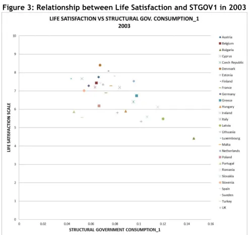
As we can observe through the figures below (Figure 1 to Figure 4), there is a clear negative correlation between the government´ weight and the indices Happiness and Life Satisfaction. In the analysis that follows, we will examine if this relationship found is robust, by the introduction of other variables typically associated in the literature with happiness.
Figure 1: Relationship between Happiness and STGOV1 in 2003
Source: Calculated based upon data from EQLS 2003 (for Happiness) and PWT (for Stgov1).
Figure 3: Relationship between Life Satisfaction and STGOV1 in 2003
Source: Calculated based upon data from EQLS 2003 (for Life Satisfaction) and PWT (for Stgov1).
Figure 4: Relationship between Life Satisfaction and STGOV1 in 2007
Additionally, in order to access the influence of a number of variables calculated by international organizations, namely those calculated by the Eurostat and used for the excessive deficit procedure by the European Commission, we also include debt (general government consolidated gross debt) and deficits (the negative of the structural balance of general government), both in percentage of potential (trend) GDP. Details on definitions and data sources of variables are in Table A.1 in the Appendix.
We estimate through Ordered Probit and OLS the following benchmark regression on life satisfaction and happiness (we name these dependent variables WB).
∑
∑
∑
(1)
Where incj,it is the household´s total net monthly income5, heaj,i,t is the individual health
conditions ranging between 1 (very good) and 5 (very bad), Eduj,i,t is the education level
(measured in ISCED levels in 2007 and in major education levels in 2003),
is the age category, which also appears squared in regressions,
is a dummy that sets 1 if the individual is unemployed in less than 12 months,
is a dummy that sets 1 if the individual is unemployed for more than 12 months,
is the number of weekly hours worked,
is the number of children,
is gender, assuming 1 for male and 2 for female,
are a set of professional categories dummies,
are a set of dummies for house features linked with the nature of the property,
is a set of dummies for marriage status (for married, divorced, widowed and never married), and finally
is one of the two structural deficits measures discussed above. The suffix _d in variables names means a dummy variable, i is the country indicator
The dummies were included in regressions but are omitted in tables to allow for better readability and because their analysis is not at the core of our analysis.
This means that in our model there are individual effects and macro-effects as in Di Tella and MacCulloch (2008) and Hessami (2011). In our case, however, macro-effects are measured by government variables. The descriptive statistics for the main variables are presented in Table 1.
Table 1: Descriptive Statistics for the main variables
Data for 2007 Data for 2003
Variable N Average Std. Dev. Min Max N Average Std. Dev. Min Max
Happiness 35380 7.336405 1.924874 1 10 25654 7.289429 1.98574 1 10 Life Satisf 35472 6.888786 2.166989 1 10 25991 6.746528 2.216835 1 10 Income 20328 1617.74 3482.832 2 250000 20498 1257.517 1296.985 75 5625 Unemp_sr 35634 0.0206825 0.1423211 0 1 26257 0.0285638 0.1665802 0 1 Unemp_lr 35634 0.0308133 0.1728139 0 1 26257 0.0360285 0.1863646 0 1 Hours Worked 29983 40.28606 11.7069 1 168 21312 41.30546 12.7853 1 140 Education 35011 3.947331 1.355418 1 7 26105 1.97376 0.7336173 1 4 Health 35570 2.330391 0.966463 1 5 26191 3.010271 1.145108 1 5 Age 35634 1.971263 0.6838658 1 3 26257 3.261721 1.273282 1 5 Mar_1 35364 0.6185665 0.4857454 0 1 26257 0.5898998 0.491861 0 1 Mar_2 35634 0.0930291 0.2904773 0 1 26257 0.0932323 0.2907632 0 1 Mar_3 35634 0.1162934 0.320581 0 1 26257 0.1213772 0.3265713 0 1 Mar_4 35634 0.1645339 0.3707645 0 1 26257 0.1866169 0.3896111 0 1 Children 35359 1.655279 1.383903 0 14 25938 1.596345 1.428991 0 15 Gender 35634 1.568895 0.4952377 1 2 26257 1.581026 0.4934005 1 2 Stgov 35634 0.0747789 0.0195345 0.0424802 0.1387043 26257 0.0809 0.0245646 0.0433155 0.1368173 Stgov1 35634 0.0747743 0.0191848 0.0416576 0.1341795 26257 0.0798974 0.0241151 0.0429177 0.145888
Notes: In order to keep the table as simple as possible, summary statistics for dummies for professional and house categories aren´t shown
The number of observations is around 26000 for 2003 and 35000 for 2007. Structural Government Expenditure (Stgov) is measured in percentage between 4% and 14%. Structural Government Expenditures with trended Government consumption (Stgov1) is measured in percentage, and oscillate between 4% and 13,4% in 2007 and between 4% and 14,5% in 2003. It is worth noting that correlations between explanatory variables rarely overcome 30% (the only exceptions being the one between children and age and the one between age and health), which implies no concern with multicollienarity.
We present both estimations from OPROB and OLS. While the OLS coefficients are more straightforward to interpret, OPROB estimations are more appropriated to estimations of equations in which the dependent variable is ordinal, i.e. that have a natural order but not
Chapter 4
Results
In this chapter, we divided the results obtained by typology of the variables studied in each pair of regressions, making the discussing into the presentation of each result. In point 4.1 we show results of the effect of structural government consumption in individual wellbeing; in point 4.2 we show the effect of alternative measures of government imbalances in individual wellbeing, by the introduction of the variables Structural Deficits and Structural Debt; in point 4.3, we show the results of regressions from differences across the income distribution and across euro zone and non-euro zone countries; in point 4.4 we show the robustness tests by introducing more macroeconomic variables such GDP per capita (in natural logarithms) and Inflation.
4.1 The effect of Structural Government Consumption in
Individual Wellbeing
In this section we will present our main results, concerning the influence of structural government expenditure in happiness or life satisfaction.
Firstly we want to analyze the individual features effects in happiness and life satisfaction. A first note is worth mentioning to say that results in happiness and life satisfaction are incredibly close. Coefficients also do not change between regressions that do not include government expenditure and those which included those variables.
From Table 2 we can observe highly significant and positive effects of income, education, number of children, being female, being married6 and health effects (note that health is
measured in inverse order, e.g. better health corresponds to lower numbers) as well as negative effects of long-run and short-run unemployment (short-run unemployment
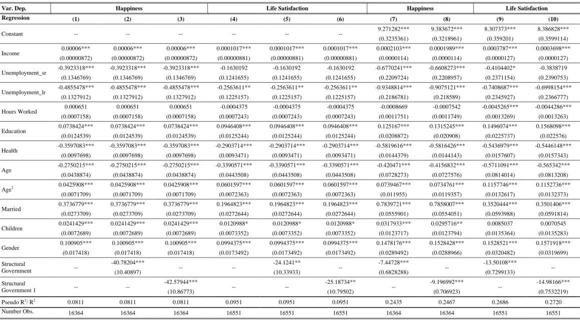
Despite of the existence of mixed effects of education and having children in the literature there are a lot of papers that also present positive effects (e.g. Di Tella et al. (2001) and Hayo and Seifert (2003) for education effects and Angeles (2009) for a positive effect of children). Columns (2)-(3), (5)-(6) and (7)-(10) test the introduction of structural government consumption in regressions and present significantly positive effects.
In Table 3 the same specifications are applied to the 2003 dataset. Despite the different sample and the different year to which the survey was applied, results are incredibly similar. We can again observe highly significant and positive effects of income, education, number of children, being male, being married and health effects as well as negative effects of long-run and short-run unemployment and hours worked (only in OLS regressions), together with a non-linear typical relationship with age.
Taking into account the OLS estimations, the effects of structural government expenditures on wellbeing mean that a 1% increase in government expenditures in percentage of GDP implies less 0.07 to less 0.42 in the happiness and/or life satisfaction scales meaning a decrease 0.7% to 4.2% of the whole scale. This also means that a 5% increase in government expenditures in % of GDP may imply a decrease in wellbeing of 4.5% to 10.5%, representing sizeable effects.
Table 2: Regressions for Wellbeing in 2007
Method Ordered Probit OLS
Var. Dep. Happiness Life Satisfaction Happiness Life Satisfaction
Regression Variables (1) (2) (3) (4) (5) (6) (7) (8) (9) (10) Constant -- -- -- -- -- -- 8.908435*** 8.924673*** 8.246053*** 8.282006*** (0.4376194) (0.4375811) (0.5228545) (0.5216138) Income 0.00000324* 0.00000324* 0.00000324* 0.00000630** 0.00000630** 0.00000630** 0.0000156*** 0.0000153*** 0.0000326*** 0.0000321*** (0.00000192) (0.00000192) (0.00000192) (0.00000280) (0.00000280) (0.00000280) (0.00000543) (0.00000538) (0.0000111) (0.000011) Unemployment_sr -0.3253964*** -0.3253964*** -0.3253964*** -0.3416401*** -0.3416401*** -0.3416401*** -0.2786565 -0.2802844 -0.5485936* -0.5509983* (0.1119254) (0.1119254) (0.1119254) (0.1182577) (0.1182577) (0.1182577) (0.2913106) (0.2908684) (0.3305154) (0.329653) Unemployment_lr -0.4114606*** -0.4114606*** -0.4114606*** -0.4750684*** -0.4750684*** -0.4750684*** -0.5654893** -0.5653744** -0.9727996*** -0.9723034*** (0.1054442) (0.1054442) (0.1054442) (0.1123546) (0.1123546) (0.1123546) (0.2850709) (0.2846065) (0.3223266) (0.3213513) Hours Worked -0.0004002 -0.0004002 -0.0004002 -0.0012928 -0.0012928 -0.0012928 -0.0062292*** -0.0061534*** -0.0094005*** -0.009265*** (0.0008242) (0.0008242) (0.0008242) (0.0008129) (0.0008129) (0.0008129) (0.0013275) (0.0013278) (0.0014764) (0.0014763) Education 0.0433858*** 0.0433858*** 0.0433858*** 0.0553147*** 0.0553147*** 0.0553147*** 0.1376807*** 0.1382745*** 0.1944765*** 0.1955898*** (0.0070014) (0.0070014) (0.0070014) (0.0070338) (0.0070338) (0.0070338) (0.0109365) (0.0109397) (0.0128151) (0.0128178) Health -0.4025707*** -0.4025707*** -0.4025707*** -0.3336939*** -0.3336939*** -0.3336939*** -0.656023*** -0.6548362*** -0.6315378*** -0.6294041*** (0.0107717) (0.0107717) (0.0107717) (0.0106194) (0.0106194) (0.0106194) (0.0168559) (0.0168625) (0.0186942) (0.018701) Age -0.4936903*** -0.4936903*** -0.4936903*** -0.4212954*** -0.4212954*** -0.4212954*** -0.7221477*** -0.7228026*** -0.6514263*** -0.6525312*** (0.0733333) (0.0733333) (0.0733333) (0.0734732) (0.0734732) (0.0734732) (0.1182457) (0.1182698) (0.1361452) (0.1362051) Age2 0.111361*** 0.111361*** 0.111361*** 0.1169483*** 0.1169483*** 0.1169483*** 0.1844776*** 0.1844057*** 0.2163215*** 0.2161609*** (0.0188314) (0.0188314) (0.0188314) (0.0190846) (0.0190846) (0.0190846) (0.0307392) (0.0307471) (0.0352877) (0.0353041) Married 0.3811907*** 0.3811907*** 0.3811907*** 0.2473287*** 0.2473287*** 0.2473287*** 0.7302369*** 0.7304895*** 0.4236384*** 0.4238679*** (0.0283387) (0.0283387) (0.0283387) (0.0277047) (0.0277047) (0.0277047) (0.0504122) (0.0504335) (0.0563734) (0.0564148) Children 0.0273806*** 0.0273806*** 0.0273806*** 0.0164** 0.0164** 0.0164** 0.057784*** 0.057781*** 0.056638*** 0.0566317*** (0.0076089) (0.0076089) (0.0076089) (0.0076766) (0.0076766) (0.0076766) (0.0123764) (0.0123695) (0.0140446) (0.0140395) 0.069363*** 0.069363*** 0.069363*** 0.0404152** 0.0404152** 0.0404152** 0.0988221*** 0.0983017*** 0.0218993 0.0211131
Table 3: Regressions for Wellbeing in 2003
Method Ordered Probit OLS
Var. Dep. Happiness Life Satisfaction Happiness Life Satisfaction
Regression Variables (1) (2) (3) (4) (5) (6) (7) (8) (9) (10) Constant -- -- -- -- -- -- 9.271282*** 9.383672*** 8.307373*** 8.386828*** (0.3235361) (0.3218961) (0.359201) (0.3599114) Income 0.00006*** 0.00006*** 0.00006*** 0.0001017*** 0.0001017*** 0.0001017*** 0.0002103*** 0.0001989*** 0.0003787*** 0.0003698*** (0.00000872) (0.00000872) (0.00000872) (0.00000881) (0.00000881) (0.00000881) (0.0000114) (0.0000114) (0.0000127) (0.0000127) Unemployment_sr -0.3923318*** -0.3923318*** -0.3923318*** -0.1630192 -0.1630192 -0.1630192 -0.6770241*** -0.6608273*** -0.4104402* -0.3838719 (0.1346769) (0.1346769) (0.1346769) (0.1241655) (0.1241655) (0.1241655) (0.2209724) (0.2208957) (0.2371154) (0.2390753) Unemployment_lr -0.4855478*** -0.4855478*** -0.4855478*** -0.2563611** -0.2563611** -0.2563611** -0.9348814*** -0.9075121*** -0.7408687*** -0.6998154*** (0.1327912) (0.1327912) (0.1327912) (0.1225157) (0.1225157) (0.1225157) (0.2186781) (0.218589) (0.2345927) (0.2366777) Hours Worked 0.000651 0.000651 0.000651 -0.0004375 -0.0004375 -0.0004375 -0.0008669 -0.0007542 -0.0045265*** -0.0044286*** (0.0007158) (0.0007158) (0.0007158) (0.0007243) (0.0007243) (0.0007243) (0.0011751) (0.0011749) (0.0013269) (0.0013263) Education 0.0738424*** 0.0738424*** 0.0738424*** 0.0946408*** 0.0946408*** 0.0946408*** 0.125167*** 0.1315245*** 0.1496074*** 0.1568098*** (0.0124539) (0.0124539) (0.0124539) (0.0125244) (0.0125244) (0.0125244) (0.0208872) (0.020908) (0.0225737) (0.022576) Health -0.3597083*** -0.3597083*** -0.3597083*** -0.2903714*** -0.2903714*** -0.2903714*** -0.5819616*** -0.5816426*** -0.5436979*** -0.5446148*** (0.0097698) (0.0097698) (0.0097698) (0.0093471) (0.0093471) (0.0093471) (0.0144379) (0.0144143) (0.0157607) (0.0157343) Age -0.2750215*** -0.2750215*** -0.2750215*** -0.3390571*** -0.3390571*** -0.3390571*** -0.420471*** -0.4156832*** -0.5711091*** -0.565342*** (0.0438874) (0.0438874) (0.0438874) (0.0443508) (0.0443508) (0.0443508) (0.0728273) (0.0727576) (0.0814014) (0.0813208) Age2 0.0425908*** 0.0425908*** 0.0425908*** 0.0601597*** 0.0601597*** 0.0601597*** 0.0739467*** 0.0734761*** 0.1157746*** 0.1152736*** (0.0071709) (0.0071709) (0.0071709) (0.0072363) (0.0072363) (0.0072363) (0.011955) (0.0119357) (0.0132617) (0.0132373) Married 0.3736779*** 0.3736779*** 0.3736779*** 0.1964823*** 0.1964823*** 0.1964823*** 0.7839721*** 0.7858007*** 0.3520444*** 0.3501406*** (0.0273709) (0.0273709) (0.0273709) (0.0272644) (0.0272644) (0.0272644) (0.0555901) (0.0554051) (0.0593988) (0.0591814) Children 0.0241429*** 0.0241429*** 0.0241429*** 0.0120988* 0.0120988* 0.0120988* 0.0317933*** 0.0295716** 0.0085037 0.0070545 (0.0072689) (0.0072689) (0.0072689) (0.0073352) (0.0073352) (0.0073352) (0.0123717) (0.0123794) (0.0135364) (0.0135283) Gender 0.100905*** 0.100905*** 0.100905*** 0.0994375*** 0.0994375*** 0.0994375*** 0.1478176*** 0.1528428*** 0.1528521*** 0.1571918*** (0.017418) (0.017418) (0.017418) (0.0173492) (0.0173492) (0.0173492) (0.0289492) (0.0288966) (0.0320482) (0.0319699) Structural Government -- -40.78204*** -- -- -24.1241** -- -7.44728*** -- -13.50108*** -- (10.40897) (10.33933) (0.6828288) (0.7299133) Structural Government 1 -- -- -42.57944*** -- -- -25.18734** -- -9.196992*** -- -14.98166*** (10.86773) (10.79502) (0.706923) (0.7532219) Pseudo R2/ R2 0.0811 0.0811 0.0811 0.0951 0.0951 0.0951 0.2435 0.2467 0.2686 0.2720 Number Obs. 16364 16364 16364 16551 16551 16551 16364 16364 16551 16551
Notes: Robust Standard deviation errors in brackets. Significance levels: ***(1%); **(5%); *(10%); for the other cases, the value is not statistic significant. Marital Status, professional, housing and country dummies included in regressions but omitted from the Table. Country dummies are excluded from OLS regressions due to collinearity.
Table 4 presents the marginal effects of regressors on wellbeing regarding ordered probit estimations, as coefficients cannot be directly interpreted as in OLS. These values may be interpreted as the probability of reporting 10 (the maximum scale of wellbeing, for both variables) due to a unit increase in each variable.
Table 4: Marginal effects for reporting maximum Wellbeing (Ordered Probit)
2007 2003
Dep. Var.
Variables Happiness Life Satisfaction Happiness Life Satisfaction
Income 0.0000005* 0.0000008** 0.000009*** 0.00001*** Unemployment_sr -0.0372*** -0.0333*** -0.0477*** -0.0154 Unemployment_lr -0.0446*** -0.0423*** -0.0556*** -0.0226*** Hours Worked -0.0001 -0.0002 0.0001 -0.00005 Education 0.0062*** 0.0070*** 0.0116*** 0.0101*** Health -0.0579*** -0.0420*** -0.0567*** -.0311*** Age -0.0710*** -0.0530*** -0.0433*** -0.0363*** Age2 0.0160*** 0.0147 0.0067*** 0.0064*** Married 0.0512*** 0.0296*** 0.0555*** 0.0203*** Children 0.0039*** 0.0021** 0.0038** 0.0012** Gender 0.0094*** 0.0051** 0.0159*** 0.0107*** Structural Government/ Structural Government1 -2.4174***/ -2.1993*** -2.7378***/ -3.0093*** -6.425***/ -6.708*** -2.5852**/ -2.6991**
Values in the table mean that additional 100 euro in the monthly income increases wellbeing in 0.005% to 0.1%, a relatively modest effect, and with higher effects in 2003 when compared to 2007.
However, being unemployed decreases the probability of reporting the highest wellbeing in from 1.5% to nearly 5%, one additional level of education increases the probability of reporting 10 in wellbeing from 0.7% to nearly 1.2% and the effect of one additional health point oscillate between 4.2% and 8% rise in the probability of reporting the highest wellbeing level. Belonging to an additional age scale decreases 5.30% to 7.10% the probability of reporting 10; being married increases 2.96% to 5.12% the probability of
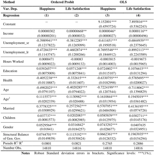
In order to answer this question we enlarge our definition of government size and test the influence of alternative variables such as government debt and deficits, calculated by the Eurostat in order to access the excessive deficits EU mechanism, which are now calculated excluding the cyclical component. If high debt and high deficits decrease wellbeing we can be more confident on our purposed explanation that relies on the negative effect macroeconomic government imbalances may have in wellbeing due to the expectations for future taxes and anticipated austerity measures.
In the following subsection we thus present results for regressions with the alternative measures of government imbalances.
4.2 The effect of alternative measures of government
imbalances in individual wellbeing
In this subsection we test the relationship between other variables that measure public finance imbalances. In this case, contrary to what has been done earlier, we choose directly available variables from the Eurostat, in particular those that serve to the excessive deficit procedure.
Firstly, we use the structural balance of general government (the negative of the deficit), calculated by the Eurostat using an adjustment based on potential GDP Excessive deficit procedure.
Table 5: Regressions for the influence of Structural Deficits on Wellbeing 2007
Method Ordered Probit OLS
Var. Dep. Happiness Life Satisfaction Happiness Life Satisfaction
Regression (1) (2) (3) (4) Constant -- -- 9.152001*** 7.895816*** (0.4593724) (0.5362243) Income 0.00000302 0.00000668** 0.0000046* 0.0000116** (0.00000201) (0.0000032) (0.0000027) (0.00000496) Unemployment_sr -0.3989941*** -0.3812285*** -0.611651*** -0.6844939*** (0.1217822) (0.1265099) (0.1950518) (0.2375645) Unemployment_lr -0.4728435*** -0.4602874*** -0.7695548*** -0.8992113*** (0.1143747) (0.1200266) (0.1846912) (0.2243589) Hours Worked 0.0000471 -0.00083 -0.0003815 -0.0019673 (0.0009022) (0.0009132) (0.0014003) (0.0015965) Education 0.0392657*** 0.0571248*** 0.0724802*** 0.1076615*** (0.0075009) (0.0075841) (0.0115107) (0.0131294) Health -0.4052238*** -0.332615*** -0.6330755*** -0.5785695*** (0.0118887) (0.011607) (0.0182998) (0.0200027) Age -0.4902025*** (0.0791107) -0.4020285*** -0.7224199*** -0.7118062*** (0.1396829) (0.0794022) (0.1207544) Age2 0.1115573*** 0.1130982*** 0.1610844*** 0.1945019*** (0.0202339) (0.020488) (0.0313954) (0.0361482) Married 0.3778325*** (0.0308929) 0.2572562*** 0.5707951*** 0.4136195*** (0.0574726) (0.0299621) (0.0484506) Children 0.037737*** (0.0081573) 0.0202083** 0.0585839*** 0.0302711** (0.0145176) (0.0082985) (0.0125975) Gender 0.0529564*** (0.01841) 0.0316842* 0.0743292*** 0.0407635 (0.0324951) (0.0184257) (0.028677) Structural Balance of Gen. Gov. 0.0744701*** (0.0149839) 0.1115192*** (0.0150424) 0.0662361*** 0.1963935*** (0.0128332) (0.0154294) Pseudo R2/ R2 0.0801 0.0821 0.2765 0.2886 Number Obs. 14810 14816 14810 14816
Notes Robust Standard deviation errors in brackets. Significance levels: ***(1%); **(5%); *(10%); for the other cases, the value is not statistic significant. Marital Status, professional, housing and country dummies included in regressions but omitted from the Table.
In Table 5 we present regressions in which we substitute the structural expenditure variable that we used earlier with the new structural balance measure, a measure that is only available for the 2007 database (as the available data begins in 2003 and we assume that an average 2003-2007 of previous years deficits is influencing wellbeing in the current year).
Table 6: Regressions for the influence of Structural Debt on Wellbeing in 2007
Method Ordered Probit OLS
Var. Dep. Happiness Life Satisfaction Happiness Life Satisfaction
Regression (1) (2) (3) (4) Constant -- -- 9.093137*** 8.086202*** (0.4421414) (0.5234773) Income 0.00000324* 0.0000063** 0.00000472* 0.0000113** (0.00000192) (0.0000028) (0.00000257) (0.00000443) Unemployment_sr -0.3253964*** -0.3416401*** -0.3930418 -0.6223497** (0.1119254) (0.1182577) (0.2722905) (0.3080155) Unemployment_lr -0.4114606*** -0.4750684*** -0.5875738** -0.9386531*** (0.1054442) (0.1123546) (0.2655505) (0.2986186) Hours Worked -0.0004002 -0.0012928 -0.0011674 -0.0029939** (0.0008242) (0.0008129) (0.0013188) (0.0014484) Education 0.0433858*** 0.0553147*** 0.0797399*** 0.1057201*** (0.0070014) (0.0070338) (0.0110163) (0.0123066) Health -0.4025707*** -0.3336939*** -0.6429343*** -0.58471*** (0.0107717) (0.0106194) (0.016932) (0.0184324) Age -0.4936903*** (0.0733333) -0.4212954*** -0.7397847*** -0.7511699*** (0.1307176) (0.0734732) (0.1148792) Age2 0.111361*** 0.1169483*** 0.1636763*** 0.2016455*** (0.0188314) (0.0190846) (0.0299124) (0.0339936) Married 0.3811907*** (0.0283387) 0.2473287*** 0.7342814*** 0.3931638*** (0.0546116) (0.0277047) (0.0490837) Children 0.0273806*** (0.0076089) 0.0164** 0.0409411*** 0.0216473 (0.0136121) (0.0076766) (0.0121408) Gender 0.069363*** (0.0171341) 0.0404152** 0.0980215*** 0.0540058* (0.0305405) (0.017178) (0.0271957) Structural Debt -0.1150848*** (0.0126166) -0.1639501*** (0.0130849) -0.0099342*** -0.0107538*** (0.0018004) (0.0018853) Pseudo R2/ R2 0.0795 0.0847 0.2778 0.2980 Number Obs. 17244 17251 17244 17251
Notes Robust Standard deviation errors in brackets. Significance levels: ***(1%); **(5%); *(10%); for the other cases, the value is not statistic significant. Marital Status, professional, housing and country dummies included in regressions but omitted from the Table.
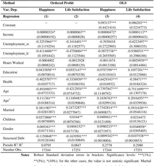
In Table 6, we use the general government consolidated gross debt calculated for the excessive deficit procedure (based on ESA 1995) – averaged from 2002 to 2007 corresponding to the 2007 database and from 1998 to 2003 corresponding to the 2003 database, which results are presented in Table 7 - as a measure of the government size.
We obtain similar values for the effects of individual effects and a strongly negative effect of debts. In this case, an additional 1% in debt/GDP would decrease wellbeing in 0.01. Thus, to decrease a one level scale in wellbeing, it would be necessary a rise in structural debt equal to 100% of GDP.
According to ordered probit analysis, an additional 1% in debt/GDP would decrease the probability of reporting the level 10 of happiness on about 1.2%. (or in the case of life satisfaction, 1.6%).
Table 7: Regressions for the influence of Structural Debt on Wellbeing in 2003
Method Ordered Probit OLS
Var. Dep. Happiness Life Satisfaction Happiness Life Satisfaction
Regression (1) (2) (3) (4) Constant -- -- 8.535198*** 6.563614*** (0.3293872) (0.3593119) Income 0.00006*** 0.0001017*** 0.0000851*** 0.0001624*** (0.00000872) (0.00000881) (0.0000132) (0.0000141) Unemployment_sr -0.3923318*** -0.1630192 -0.6122368*** -0.3183591 (0.1346769) (0.1241655) (0.215857) (0.2248268) Unemployment_lr -0.4855478*** -0.2563611** -0.8104646*** -0.5483238** (0.1327912) (0.1225157) (0.2140113) (0.2227633) Hours Worked 0.000651 -0.0004375 0.0009517 -0.0008534 (0.0007158) (0.0007243) (0.0011747) (0.0012954) Education 0.0738424*** 0.0946408*** 0.14637*** 0.1893028*** (0.0124539) (0.0125244) (0.0205707) (0.0219483) Health -0.3597083*** -0.2903714*** -0.5698401*** -0.4995031*** (0.0097698) (0.0093471) (0.014979) (0.0158812) Age -0.2750215*** (0.0438874) -0.3390571*** -0.4173913*** -0.5818934*** (0.0783632) (0.0443508) (0.0713384) Age2 0.0425908*** 0.0601597*** 0.0643098*** 0.1021738*** (0.0071709) (0.0072363) (0.0117675) (0.0128443) Married 0.3736779*** (0.0273709) 0.1964823*** 0.8112679*** 0.389683*** (0.0566351) (0.0272644) (0.0540411) Children 0.0241429*** (0.0072689) 0.0120988* 0.0367935*** 0.0140728 (0.0128985) (0.0073352) (0.0119597) Gender 0.100905*** (0.017418) 0.0994375*** 0.1500234*** 0.1635632*** (0.0307356) (0.0173492) (0.0283905) Structural Debt -0.0247495*** (0.0063169) -0.0146402** (0.0062747) 0.0006326 0.0082016*** (0.001095) (0.0011125) Pseudo R2/ R2 0.0811 0.0951 0.2833 0.3347 Number Obs. 16364 16551 16364 16551
Notes Robust Standard deviation errors in brackets. Significance levels: ***(1%); **(5%); *(10%); for the other cases, the value is not statistic significant. Marital Status, professional, housing and country dummies included in regressions but omitted from the Table.
Table 7 confirms the results obtained so far for the influence of debt in the wellbeing measure in 2003, specifically in the Ordered Probit regressions. There is a quantitatively smaller positive effect of debt in the OLS regression for life satisfaction. Moreover, with a 1% (of GDP) increase in structural debt, the probability of reporting 10 in wellbeing will decrease on 0.39% (if wellbeing is measured by happiness) or 0.16% (if wellbeing is measured by life
4.3 Differences across the income distribution and across
countries from the Euro zone and others
In this section we want to evaluate if the negative effect of government imbalances in wellbeing is different between different income levels and differs between euro zone countries and non-euro countries.7
The first issue is important as the literature points out that the eventual positive effects of government size in wellbeing may be due welfare policies, thus affecting essentially the poorest in the society. We consider high-income people that presented a monthly income that is above the fourth quartile and low-income people those who earn a monthly income that is below the median.
The second issue is important to access potential differences in the effect of government size on wellbeing between the countries of the Eurozone and countries out of the Eurozone. It would be reasonable to assume that the tighter budgetary limits under the euro area would imply a lower effect of government structural deficits/expenditures in wellbeing. In this section, due to similarities in the results between several tested specifications, we will not present results for Life Satisfaction and the influence of structural government (Stgov). However, these regressions are available upon request.
Table 8 analyses the differences from the consideration of a sample with the Euro countries and another with other European Countries for the 2007 data. Table 9 does the same but for the 2003 data. Table 10 analyses the differences from the consideration of a sample with the richest people in the sample and a sample of the poorest people in the sample. Table 11 does the same but for the 2003 data.
7As in this case we are dealing with more homogeneous (and smaller) samples, we did not introduce
country dummies. Also some of the ordered probit regressions have convergence problems when country dummies are included.
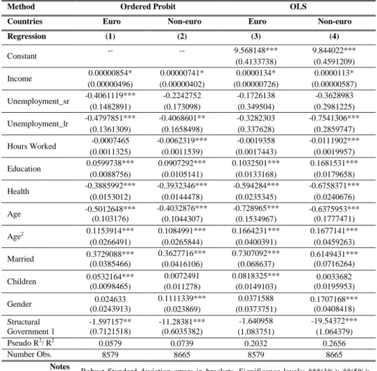
Table 8: Regressions for Wellbeing 2007 (Happiness) - euro versus non-euro countries
Method Ordered Probit OLS
Countries Euro Non-euro Euro Non-euro
Regression (1) (2) (3) (4) Constant -- -- 9.568148*** 9.844022*** (0.4133738) (0.4591209) Income 0.00000854* 0.00000741* 0.0000134* 0.0000113* (0.00000496) (0.00000402) (0.00000726) (0.00000587) Unemployment_sr -0.4061119*** -0.2242752 -0.1726138 -0.3628983 (0.1482891) (0.173098) (0.349504) (0.2981225) Unemployment_lr -0.4797851*** -0.4068601** -0.3282303 -0.7541306*** (0.1361309) (0.1658498) (0.337628) (0.2859747) Hours Worked -0.0007465 -0.0062319*** -0.0019358 -0.0111902*** (0.0011325) (0.0011539) (0.0017443) (0.0019957) Education 0.0599738*** 0.0907292*** 0.1032501*** 0.1681531*** (0.0088756) (0.0105141) (0.0133168) (0.0179658) Health -0.3885992*** -0.3932346*** -0.594284*** -0.6758371*** (0.0153012) (0.0144478) (0.0235345) (0.0240676) Age -0.5012648*** (0.103176) -0.4032876*** -0.728965*** -0.6375953*** (0.1777471) (0.1044307) (0.1534967) Age2 0.1153914*** 0.1084991*** 0.1664231*** 0.1677141*** (0.0266491) (0.0265844) (0.0400391) (0.0459263) Married 0.3729088*** (0.0385466) 0.3627716*** 0.7307092*** 0.6149431*** (0.0716264) (0.0416106) (0.068637) Children 0.0532164*** (0.0098465) 0.0072491 0.0818325*** 0.0033682 (0.0195953) (0.011278) (0.0149103) Gender 0.024633 (0.0243913) 0.1111339*** 0.0371588 0.1707168*** (0.0408418) (0.023869) (0.0373751) Structural Government 1 -1.597157** (0.7121518) -11.28381*** (0.6035382) -1.640958 -19.54372*** (1.083751) (1.064379) Pseudo R2/ R2 0.0579 0.0739 0.2032 0.2656 Number Obs. 8579 8665 8579 8665 Notes
Robust Standard deviation errors in brackets. Significance levels: ***(1%); **(5%); *(10%); for the other cases, the value is not statistic significant. Marital Status, professional and housing dummies included but omitted from the Table.
There are interesting differences between effects within the Euro zone and effects outside the Eurozone: having children seems to contribute to wellbeing within the countries of the Euro (in opposition to what happens in countries outside the Euro zone) and being male seems to increase wellbeing in countries out of the Euro zone while this is not a significant determinant of wellbeing in the Euro zone.
Table 9: Regressions for Wellbeing 2003 (Happiness) - euro versus non-euro countries
Method Ordered Probit OLS
Countries Euro Non-euro Euro Non-euro
Regression (1) (2) (3) (4) Constant -- -- 9.955948*** 9.107915*** (0.353643) (0.5121071) Income 0.0001229*** 0.00012*** 0.0001999*** 0.0001949*** (0.00000969) (0.0000119) (0.0000145) (0.0000187) Unemployment_sr -0.4393708*** -0.3627788 -0.6953463*** -0.3082216 (0.1554018) (0.2397473) (0.2338912) (0.335646) Unemployment_lr -0.5543784*** -0.4549501* -0.9913455*** -0.4658808 (0.1565406) (0.234553) (0.2416252) (0.3240451) Hours Worked 0.000684 -0.0010077 0.0006766 -0.0022035 (0.0009507) (0.0010245) (0.0014689) (0.0018478) Education 0.0191021 0.1079797*** 0.0477642* 0.2207662*** (0.0173121) (0.0175302) (0.0280206) (0.0309773) Health -0.3540828*** -0.359244*** -0.5361274*** -0.6239364*** (0.0129667) (0.0136111) (0.0189145) (0.022532) Age -0.3052281*** (0.0599948) -0.2333526*** -0.4681171*** -0.3756706*** (0.1156225) (0.0643621) (0.0915937) Age2 0.0486157*** 0.0435429*** 0.0754449*** 0.0710835*** (0.0099402) (0.0102383) (0.0153085) (0.0185004) Married 0.3384212*** (0.0358512) 0.2996646*** 0.4953292*** 0.5190673*** (0.0755466) (0.0420085) (0.0567593) Children 0.0172804* (0.0095494) 0.0247579** 0.0254036* 0.0353257* (0.0206338) (0.0114784) (0.0151994) Gender 0.034055 (0.0239688) 0.167137*** 0.0412643 0.274095*** (0.0448405) (0.0251717) (0.0373859) Structural Government 1 -5.522587*** (0.674037) -5.268*** (0.5853156) -8.029281*** -9.919494*** (1.098872) (1.076152) Pseudo R2/ R2 8718 7646 0.2106 0.2626 Number Obs. 0.0610 0.0738 8718 7646
Notes Robust Standard deviation errors in brackets. Significance levels: ***(1%); **(5%); *(10%); for the other cases, the value is not statistic significant. Marital Status, professional and housing dummies included but omitted from the Table.
In 2003 some differences between the Euro zone and other countries also arise. Unemployment is now clearly more important as a determinant of wellbeing in the Euro countries. Now, education, having children and being male are stronger determinants of welfare out of the euro zone than with the euro countries. Concerning the effect of structural government expenditures, we note that the 2007 results does not confirm in 2003. In this year both groups of countries present a significantly negative effect, with no relevant distinction between them.
There are also interesting differences in the determinants of wellbeing between the richest and the poorest. In fact, for high-income earners, income and unemployment are not statistically significant in the explanation of wellbeing, a quite intuitive result. It seems that there is also a less significant effect of structural government expenditures in high-income agents than in the poorest. This indicates that our effect is different from the potential positive effect of welfare state expenditures in the wellbeing of the poorest, supporting our approach on the analysis of the influence of structural expenditures, which excludes
counter-cyclical expenditures such as unemployment subsidies or some measures for the alleviation of poverty.
Table 10: Regressions for Wellbeing 2007 (Happiness) - differences between High-Income and Low-Income earners
Method Ordered Probit OLS
Individuals High-Income Low-Income High-Income Low-Income
Regression (1) (2) (3) (4) Constant -- -- 8.686379*** 7.777394*** (0.7025152) (0.5805595) Income -0.0000000527 0.0006612*** 0.000000661 0.0012422*** 0.00000164 0.0000562 (0.00000190) 0.0001007 Unemployment_sr -0.2765138 -0.2973768* -0.2006755 -0.1709532 0.1918318 0.1584862 (0.3407431) 0.4072372 Unemployment_lr -0.1027897 -0.4291308*** -- -0.4338661 0.2246365 0.1509682 0.3979505 Hours Worked -0.0003298 -0.0026463** -0.0011353 -0.0052094** 0.0016151 0.0011489 (0.0020309) 0.0020842 Education 0.0247298** 0.0936287*** 0.0416819*** 0.1713247*** 0.0125276 0.011179 (0.0157975) 0.0202102 Health -0.3417024*** -0.3938565*** -0.4229169*** -0.7245214*** 0.0202804 0.0153753 (0.0272783) 0.0268952 Age -0.6054246*** 0.1511379 -0.3814767*** -0.7472762*** -0.649254*** 0.1980303 0.1106464 (0.1884626) Age2 0.1522419*** 0.1008702*** 0.1869221*** 0.1729274*** 0.0422918 0.0265799 (0.0532503) 0.0479469 Married 0.3001342*** 0.0587513 0.298259*** 0.7497929*** 0.5259276*** 0.0771083 0.0424206 (0.1400172) Children 0.0634793*** 0.0148166 0.0252305** 0.0708687*** 0.044782** 0.0200138 0.0109304 (0.0183725) Gender 0.0698762** 0.032578 0.1055287*** 0.0652152 0.1938793*** 0.0460938 0.0254113 (0.0410735) Structural Government 1 -2.947929** 1.183408 -5.319798*** 0.6141005 -2.101765 -9.414843*** (1.456999) 1.127548 Pseudo R2/ R2 0.0371 7874 0.1119 0.2158 Number Obs. 4821 0.0564 4821 7874
Notes Robust Standard deviation errors in brackets. Significance levels: ***(1%); **(5%); *(10%); for the other cases, the value is not statistic significant. Marital Status, professional and housing dummies included but omitted from the Table. Unemployment_lr was excluded in column (3) due to collinearity.
Table 11: Regressions for Wellbeing 2003 (Happiness) - differences between High-Income and Low-Income earners
Method Ordered Probit OLS
Individuals High-Income Low-Income High-Income Low-Income
Regression (1) (2) (3) (4) Constant -- -- 9.23637*** 8.254977*** (0.4489854) (0.6469352) Income 0.0000645*** 0.000616*** 0.0000706*** 0.0012761*** 0.0000159 0.0000795 (0.000019) (0.0001521) Unemployment_sr -0.1905951 -0.4808955** -0.2462002 -0.4703156 0.309707 0.2309623 (0.3645275) (0.5008158) Unemployment_lr -0.2081445 -0.5108766** -0.3461647 -0.5432214 0.3253696 0.226716 (0.3849695) (0.4940437) Hours Worked 0.0023433 0.0010261 0.0025536 0.0016376 0.0016229 0.0009959 (0.0019382) (0.0019042) Education -0.0472612* 0.1164895*** -0.0458441 0.235442*** 0.0265393 0.0183443 (0.0313681) (0.0355814) Health -0.3588903*** -0.3460005*** -0.4143546*** -0.6571576*** 0.0189809 0.0146213 (0.0220163) (0.0261736) Age -0.2934693*** 0.1025129 -0.1926082*** -0.3745665*** -0.3456678*** (0.1252738) 0.0654079 (0.121873) Age2 0.0457528*** 0.0327819*** 0.0591792*** 0.0589908*** 0.0170558 0.0101963 (0.0202666) (0.019591) Married 0.3761402*** 0.0612621 0.3334035*** 0.92045*** 0.7293897*** (0.0759624) 0.0451398 (0.1712325) Children 0.055296*** 0.0172589 0.0047346 0.0610156*** 0.0097042 (0.0211193) 0.0109152 (0.0207616) Gender 0.0760193** 0.0361744 0.1007601*** 0.0874909** 0.1807097*** (0.0502694) 0.0260712 (0.042956) Structural Government 1 -3.373533** 1.374285 -3.191033*** 0.5306012 -3.39242** -5.952919*** (1.701827) (1.022862) Pseudo R2/ R2 0.0533 0.0485 0.1552 0.1872 Number Obs. 3809 7191 3809 7191
Notes Robust Standard deviation errors in brackets. Significance levels: ***(1%); **(5%); *(10%); for the other cases, the value is not statistic significant. Marital Status, professional and housing dummies included but omitted from the Table.
In 2003 almost all the results of 2007 are confirmed but in this case also Education is a worse predictor of wellbeing for the richest than for the poorest. The interesting conclusion according to which structural government expenditures affect more the wellbeing of the poorest than that of the richest remains also in 2003.
4.4 Robustness tests for the introduction of more
macroeconomic variables
As previous literature also included other macroeconomic variables (e.g. Hessami, 2010) as determinants of happiness, we want to further test our result against the introduction of other macroeconomic variables. The most important macroeconomic variables to relate with happiness are GDP per capita (which in fact can be a substitute to the consideration of average income, which has been mentioned above in footnote 5) and inflation. Previous literature had found positive effects of GDP per capita and negative effects of inflation.