Pedro Alexandre Velez Fernandes

Setembro , 2016

Pedro Alexandre Velez Fernandes

e de Computadores

Capac ity o f a Massive MIMO-OFDM system using

Millimetric Waves

Disse rtação para o btenção do Grau de Me stre em

Engenharia Eletrotécnica e de Computadores

Orie ntado r: Rui Dinis, Profe sso r Asso ciado com agregação , FCT-UNL

Co -o rie ntado r: Paulo Mo nte zuma-Carvalho , Profe sso r Auxiliar, FCT-UNL

Júri:

Presidente : Doutor Jo ão Pedro Abreu de Olive ira

Argue ntes: Doutor Luís Filipe Loure nço Bernardo

Capacity of a Massive MIMO-OFDM system using Millimetric waves

Copyright © Pedro Alexandre Velez Fernandes, Faculdade de Ciências e Tecno-logia, Universidade Nova de Lisboa.

Acknowledgement

My deepest gratitude to professor Rui Dinis and Paulo

Montezuma-Car-valho for accepting me in this very interesting project and for always being there

offering suggestions and guidance, without them this thesis would not have been

completed. My special thanks to João Guerreiro, for his help, his advises, and for

his great patience. Finally, I would like to give my heartfelt to my parents, brother

Abstract

In modern day society, wirelesses communications are fundamental to the communications worldwide. But with the saturation of the usable spectrum for communications, the need for capacity is one of the most important challenges faced nowadays.

With the development of technology, there is a much great need for quality of the service and bigger data streams. Increasing the capacity of a telecommuni-cation system will allow to cope with that need.

The solution for the need for capacity, can be solved with the use of massive multiple input multiple output (MIMO) techniques, since MIMO system ap-proach have already shown to increase the capacity of a wireless system.

The implications of this approach will make systems more complex and more energy consuming, in order to sustain the massive MIMO system. But such implementation combined with millimeter waves will allow the increase of the capacity of a system.

Resumo

Na sociedade moderna, comunicações sem fios, são fundamentais para as comunicações a nível global. Mas com a saturação do espectro passível de ser utilizado, a necessidade por capacidade é um dos desafios mais importantes para os dias de hoje.

Com o desenvolvimento de tecnologia, existe cada vez mais uma necessi-dade de qualinecessi-dade de serviço e de maior quantinecessi-dade de dados. Aumentar a ca-pacidade de um sistema de telecomunicações irá permitir cobrir essa necessi-dade.

A solução para a necessidade de capacidade, pode ser resolvida com o uso de técnicas massive input multiple output (Massive MIMO). Uma vez que a apro-ximação com sistemas MIMO, já demonstrou aumentar a capacidade de um sis-tema sem fios.

As implicações desta abordagem fará com que os sistemas tenham que se tornar mais complexos, e que consumam mais energia, de forma a conseguir sus-ter o sistema massive MIMO. Porém tal implementação combinada com ondas milimétricas irá permitir o aumento da capacidade do sistema.

Index of Contents

ABSTRACT ... IX

RESUMO ... XI

INDEX OF CONTENTS ... XIII

LIST OF FIGURES ... XV

LIST OF PUBLICATIONS ... XVII

LIST OF ABBREVIATIONS ... XVIII

1 - INTRODUCTION ... 1

1.2–OFDMMULTICARRIER TRANSMISSION ... 3

1.3-MIMO ... 4

1.4-CHANNEL ... 5

1.4.1 – Multipath Effect ... 5

1.4.3 – Rayleigh Fading ... 7

1.4.4 – Doppler Fading ... 7

1.4.5 – Slow and fast Fading ... 9

1.5–OVERVIEW OF MASSIVE MIMO ... 10

1.6CHANNEL CAPACITY ... 11

2-EXISTING TECHNIQUES ...13

2.1–OFDM TECHNIQUES ... 13

2.2–MIMOSYSTEM ... 16

2.3–MIMO-OFDMSYSTEM ... 18

2.4.1 – Selection Diversity ... 19

2.4.2 – Alamouti Scheme ... 20

2.4.3 – Alamouti Scheme with two transmitter antennas one receiver antenna ... 20

2.4.4 – Alamouti Scheme two transmitter antennas two receiver antenna ... 22

2.4.5 – Beamforming technique ... 23

2.4.6 – Maximal-ratio combining (MRC) ... 25

CAPACITY OF THE SYSTEM ...27

3.1CAPACITY OF A LINEAR SISO SYSTEM ... 32

3.2CAPACITY OF A NONLINEAR SISO SYSTEM ... 34

3.3CAPACITY OF A LINEAR MIMOSYSTEM ... 37

3.4CAPACITY OF A NONLINEAR MIMOSYSTEM ... 38

CONCLUSION ...45

List of Figures

Fig 1.1- Multipath effect……….……..…….. 7

Fig 1.2 - Doppler effect ……….…………..…… 10

Fig 1.3 – SISO system..……….…….…13

Fig 2.1 –Basic OFDM transmitter……….….….15

Fig 2.2 –Basic OFDM Receiver………..….….16

Fig 2.3 – Signal with Cyclic prefix …..………..….….16

Fig 2.4 –MIMO structure..………..….…17

Fig 2.5- Basic structure MIMO-OFDM………..….…19

Fig 2.6 – Basic structure of transmit selection diversity………... 21

Fig 2.7 Basic structure of Maximal-ratio Receiver Combining………..…… 26

Fig 3.1 Linear SISO System………..…... 34

Fig 3.2 Linear SISO System with SVD………..……..34

Fig 3.3 – Non Linear SISO system………...……..36

Fig 3.4 – Non Linear SISO system with SVD………...…….. 37

Fig 3.5- Evolution of capacity of the linear MIMO-OFDM for different values of T……….……..40

Fig 3.7 - Evolution of the capacity for nonlinear channel for 𝑆_𝜎𝑀

𝑥 = 0,5, q = 1, R = 8

and different values of T . ………....……44

Fig 3.8. Evolution of the degradation for an SSPA with different saturation levels

and different values of q. ………...…. 45

Fig 3.9- Evolution of the channel capacity for R = 8, T = 32, different saturation

List of publications

This thesis consists of an overview and of the following publications which are

referred to in the text by their Roman numerals.

I

Nonlinear Massive MIMO-OFDM Systems ”, In Proc. of IEEE VTC'16 (Fall),

List of Abbreviations

5G - 5𝑡ℎ Generation

4G - 4𝑡ℎ Generation

3G - 3𝑡ℎ Generation

VLSI - Very-Large-Scale Integration

OFDMA - Orthogonal Frequency-Division Multiple Access

FDE - Frequency-Domain Equalization

MIMO - Multiple-Input Multiple-Output ADSL - Asymmetric Digital Subscriber Line

SISO - Single-Input-Single-Output

ISI - Inter Symbol Interference

SNR - Signal-to-Noise Ratio

AWGN - Addictive White Gaussian Noise

NLOS - Non-Line-Of-Sight

PDF - Probability Density Function

BS - Base Stations

TDD - Time Division Duplexing

FDD - Frequency Division Duplexing

SISO - OFDM - Single Input Single Output Orthogonal Frequency-Division

IFFT - Inverse Fast Fourier Transformation

S/P - Serial to Parallel

P/S - Parallel to Serial

MRC - Maximal-Ratio Combining

LLR - Log-Likelihood Ratio

BPSK - Binary Phase-Shift Keying

STBC - Space Time Block Code

SSPA - Solid State Power Amplifier

1 - Introduction

Wireless systems are one of the most used and more important

communi-cation systems in the current days. In the past years, they have become the

elec-tion choice for millions of users around the world, having democratize

commu-nications. Such development allowed the world to be more connected than ever,

connecting the most remote zones of the world to the rest of the world. Massive

MIMO have the capability of expanding even more its influence, if they can

in-crease the quality and capacity. If such objectives are obtained the wireless

sys-tems will be able to become the most important communication system in use,

substituting even optical fiber cable in some cases.

The 5𝑡ℎ generation(5G) are the proposed next generation

telecommunica-tion standards, that will substitute the present 4𝑡ℎ generation (4G) systems. 5G

systems are being planned to allow greater capacity. With 5G systems, and

there-fore the increase in capacity, it will be possible to have more mobile broadband

users per area, at the same time will allow the users to consume higher data

quan-tities. That is possible thanks to the spectral efficiency, that 5G will allow. The use

of 5G will also allow a better coverage and reduced latency.

1.1 - Overview of a Wireless system

Wireless communication systems have been a topic of study since 1960. The

development of wireless communication technology is due to several reasons.

First the demand by users for wireless connectivity increased in the past years.

Second the development of Very-large-scale integration (VLSI) technology,

ena-bled the implementation of small area circuits, low power signal processing and

coding algorithms [1]. Third, the demand of high bit rates and high mobility

in-creased in the last years with the advance of smartphones and PDA’s or tablets.

In the 4G systems the spread spectrum radio technology used in 3G was

abandoned and replaced with Orthogonal Frequency-Division Multiple

Ac-cess (OFDMA) multicarrier transmission and other frequency-domain

equaliza-tion (FDE) schemes, making possible to transfer very high bit rates despite

multi-path propagation effects and channel selectivity. The peak bit rate was further

improved by smart antenna arrays for multiple-input multiple-output (MIMO)

communications.

Wireless communication systems enabled the development of several

ap-plications, such as smart phones with Internet connection, industrial sensor

net-works, smart homes, wireless controlled cars, as several other applications in

terms of autonomous health, security and leisure systems. The adaptability of the

wireless systems as well as its reliability, allowed the expansion and

develop-ment of new technology all across the globe, , at an accessible quality-price

rela-tion, democratizing the data and information access.

However, there are two significant technical challenges in supporting these

applications: first is the phenomenon of fading due to time variation of the

ef-fect like the path loss by distance attenuation and shadowing by obstacles.

Sec-ond, since wireless transmitter and receiver need to communicate over the air,

there is significant interference between them.

Overall, the challenges are mostly because of limited availability of radio

frequency spectrum and a complex time-varying wireless environment (fading

and multipath). In nowadays, the key goal in wireless communication is to

in-crease data rate and improve transmission reliability. In other words, the

increas-ing demand for higher data rates implies better quality of service, fewer dropped

calls, higher network capacity and user coverage calls. This can only be achieved

by techniques that improve spectral efficiency and link reliability and more

tech-nologies in wireless communication were introduced, like OFDM and MIMO. [2]

1.2

–

OFDM Multicarrier transmission

OFDM is a method of digital modulation in which the data stream is split

into N parallel streams of reduced data rate, each of them transmitted on separate

subcarriers. In short, it is a kind of multi-carrier digital communication method.

OFDM has been around for about 40 years and it was first conceived in the 1960s

and 1970s to minimize interference among channels near each other in frequency

[3].

OFDM is employed in wireless and fixed communication systems

stand-ards such as asymmetric digital subscriber line (ADSL) broadband and digital

audio and video broadcasts. OFDM is also successfully applied to a wide variety

of wireless communication due to its high spectral efficiency and its robustness

In conclusion OFDM has been proposed as a transmission method to

sup-port high-speed data transmission over wireless links in multipath environments

[5].

1.3- MIMO

MIMO has been developed for many years for wireless systems. One of the

earliest MIMO implementations on wireless communications applications came

in mid 1980 with the breakthrough developments by Jack Winters and Jack Saltz

of Bell Laboratories [6]. They tried to send data from multiple users on the same

frequency/time channel using multiple antennas both at the transmitter and

re-ceiver. After such experience several evolutions on the MIMO systems have been

developed all across the world.

Now the interest in MIMO technology has aroused because when

com-pared with Single-input-single-output (SISO) system, MIMO provides enhanced

system performance under the same transmission conditions. First, a MIMO

sys-tem greatly increases the channel capacity, which is proportional to the total

number of transmitter and receiver arrays. Second, MIMO system provides the

advantage of spatial diversity: each one transmitting signal is detected by the

whole detector array, which not only improves system robustness and reliability,

but also reduces the impact of inter symbol interference (ISI) and channel fading,

since each signal determination is based on N detected results. In other words,

spatial diversity offers N independent replicas of the transmitted signal. Third,

the Array gain is also increased, which means a signal-to-noise ratio (SNR) gain

the increased complexity in both the transmitter and receiver. With the use of

Massive MIMO the problem escalates, since the implementation of massive

MIMO is far more complex than the one used with MIMO, therefore it will

re-quire more energy in order to allow the system to work at is full potential.

1.4- Channel

In wireless communications there are several distortion effects and

impair-ments in the communication channels. One cause is the multi-path effect, in

which the signal will be reflected on several objects such as cars, buildings and

others. Therefore the receiver antennas will receive the same signal several times,

because the signal will follow several different paths and will arrive at different

times (called time dispersion). Such effect creates multipath fading and

inter-symbolic interference. Fading due to multi-path spread is called frequency

selec-tive fading.

Other cause is the relative motion between receiver and transmitter which

originates the Doppler effect as well as slow and fast fading.

A third cause is the signal attenuation, since the power received depends

on the path length that the transmitted signal has to travel. When there is an

ob-stacle between the transmitter and the receivers such as buildings, the most likely

case to happen is the attenuation of the power of the signal. Finally, the noise that

the system experiences, such as thermal noise in the receiver, atmospheric noise

or noise resulting of the interference of wireless carriers, transmitters and

sys-tems. These types of noise are independent from the transmitted signals and from

the channel. Such noises can be described as Addictive White Gaussian Noise

(AWGN), although not all of types of noise can be described as AWGN.

1.4.1 – Multipath Effect

In conventional wireless systems such as SISO, where there is one

be described as the signal being reflect in inanimate objects creating several

rep-licas of the original signal. The several reprep-licas will be perceived at the receptor

with different phases, amplitudes and angles.

In figure 1.1 it can be seen the representation of the multipath effect, where

the signal is reflected on buildings, the different colors serve as a demonstration

of the alterations that the signal is submitted, when it is reflected.

Fig 1.1- Multipath effect

The multipath effect may cause several interferences, creating an increase

in number of errors, lowering the quality of the signal and therefore a reduction

in data speed.

Regarding the fading we can have two different: flat fading and frequency

selective fading. When the transmission occurs, the signal can be affected on its

amplitude and phase. If the transmitted signal experiences an alteration in all of

its spectral components with the same amplitude gains and phase shifts, the

channel is called flat fading channel. Frequency selective fading will induce

inter-symbol interference, which can be compensated by digital processing. Assuming

a single transmitted impulse, whose time duration 𝑇_𝑚 is the duration between

the first and last received component that possesses the maximum delay spread,

therefore the coherence bandwidth 𝑓_𝑐 is _𝑇1

𝑚. As we all know, symbol time is 𝑇𝑠. A

fading if 𝑇_𝑚<𝑇_𝑠 . [7]. In this particular case, the transmitted signal bandwidth is

much smaller than the channel’s coherent bandwidth. Flat fading channel occurs

in many wireless environments and causes deep fades. The amplitude

distribu-tion of flat fading is either Raleigh distribudistribu-tion or Ricean distribudistribu-tion.

1.4.3 – Rayleigh Fading

The Rayleigh distribution is used to model the multipath fading effect, in a

case where non-line-of-sight (NLOS) transmission occurs, which means that the

signal perceived at the receiver is the result of the reflections. In this case, the

probability density function (PDF) of fading amplitude of the 𝑖𝑡ℎ path 𝑎_𝑖 is given

by

𝑓𝛼𝑖(𝛼𝑖) = 2𝛼𝑖

Ω_𝑖 𝑒𝑥𝑝 (−

𝛼_𝑖2

Ω_𝑖) , 𝛼𝑖 ≥ 0, (1.1)

where Ω_𝑖= E [𝑎_𝑖2 ] and exp[·]denotes the expectation of its argument [8].

In the case where it exists line of sight, the Rician fading is more applicable.

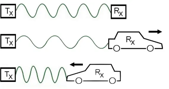
1.4.4 – Doppler Fading

In wireless communications where there is relative movement of the

ele-ments of the system i.e. the receiver moves away or closer to the transmitter, the

Doppler effect (shift) may occur. The Doppler effect is the change in

fre-quency/wavelength due to relative motion to the source of the waves. The

Dop-pler effect is directly proportional to the magnitude of the relative speed and is

modeled here as a contribution to the carrier frequency. For waves which do not

require a medium, only the relative difference in velocity between the observer

representation of the Doppler effect, showing the effect that the movement of the

receptor to the transmitter has on the frequency of the transmitted wave. It is

possible to observe the stationary case, the case where the receiver is moving

away from the transmission source and the case where the receiver is moving

towards the transmission source.

Fig. 1.2 - Doppler effect

Because the detected frequency increases as the receiver is moving toward

the observer, the source's velocity must be subtracted when motion is moving

toward the observer. Therefore when receiver is moving away from the observer

the detected frequency decreases, so the source’s velocity must be added when

the motion is moving away from the observer.

The phase difference between two transmission paths is given by

𝛥𝜙 =2𝜋𝛥𝑙_𝜆 =2𝜋𝛥𝑡_𝜆 cos 𝜃. (1.2)

The Doppler shift is given by

If a pure sinusoid wave is transmitted, a range of frequencies adjacent to

this sinusoid frequency will be received. The Doppler shift broadens the

spec-trum of the received signal by spreading the basic specspec-trum in frequency domain.

If the signal spectrum is wide enough compared to this spreading, the effect is

not noticeable, otherwise, distortion will occur.

Both multi-path fading and Doppler effects can impair the reception of the

transmitted signal. It is also well known that ISI happens when multiple paths

are received with various delays and co-channel users create distortion to the

target user. And thermal noise is electronic white noise that definitely needs to

be counted in. Diversity, as stated by Proakis [10] is an effective way to improve

error rate performance in fading channels. MIMO OFDM is introduced as a

scheme in wireless communications to offer diversity, capacity and array gain

[11]

1.4.5 – Slow and fast Fading

The Doppler effect fading effect creates a spread, that can be divided in Fast

Fading and slow fading. In wireless communication, a channel can be time

vary-ing and those dynamic channels are characterized as slow or fast fadvary-ing channels.

Fast fading channel changes significantly during the duration of a symbol. And

when the channel varies rapidly, it distorts the symbol’s amplitude and phase

erratically over its interval. On the other hand, slow fading occurs when the

chan-nel changes much slower than one symbol duration. This does not imply that the

effects of the channel can be neglected, but it is possible to track the changes in

the channel to appropriately compensate for channel dynamics. We define

coher-ence time 𝑇_𝑐 of the channel as the period of time over which the fading process is

correlated. 𝑇_𝑐 is closely related to Doppler spread 𝑓_𝑑 as:

If the symbol time duration 𝑇_𝑠 is smaller than 𝑇_𝑐, the fading is slow fading,

otherwise, the channel fading is considered fast fading [12].

1.5

–

Overview of Massive MIMO

Since MIMO gains increase with the number of antennas, there is interest

in MIMO systems with a huge number of antennas, usually denoted massive

MIMO schemes. Massive MIMO schemes where a given base stations (BS) with

several tens or even hundreds of antenna elements communicates

simultane-ously with several tens of MTs are being proposed for 5G systems [13].

Although the potential capacity gains can be very high, the implementation

complexity of MIMO schemes grows very fast with the number of antenna

ele-ments. Therefore, massive MIMO schemes cannot be regarded as a scaled version

of conventional MIMO schemes, and low-complexity implementations are

re-quired [14].

In massive MIMO the number of transmitters is large, so a time division

duplexing (TDD) is preferable in opposing to a frequency division duplexing

(FDD), because that with TDD adding more antennas does not affect the

re-sources needed for the channel estimation. Because of the large number of BS

antennas and the number of users are large, the signal processing at the terminal

end must deal with large dimensional matrices/vectors. Thus, simple signal pro-cessing is preferable. In Massive MIMO, linear propro-cessing (linear combining schemes in the uplink and linear precoding schemes in the downlink) is nearly optimal.

as large as desired with no increase in the channel estimation overhead. Further-more, the signal processing at each user is very simple and does not depend on other users' existence, i.e., no multiplexing or de-multiplexing signal processing is performed at the users. Adding or dropping some users from service does not affect other users activities.[15]

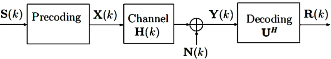
1.6 Channel Capacity

Capacity of systems has been widely studied across the years. The channel

capacity is defined as the tight upper bound on the rate at which information can

be reliably transmitted over a communication channel. For a linear single input

single output Orthogonal Frequency-Division (SISO- OFDM) transmission in

ideal additive white Gaussian noise AWGN channels, the capacity is [16]

𝐶 = 𝐵 log2(1 + 𝑆𝑁𝑅). (1.5)

By the Shannon Hartley theorem, where C represents the capacity, B the

bandwidth and SNR represents the signal to noise ratio that is _𝑁𝑆. The

representa-tion of the SISO system being considered for this results can be seen in Fig 1.3

Fig 1.3 – SISO system

This model will serve as the base for the study of the capacity of massive

MIMO with linear and non-linear effects. Since that after the precoding and

de-coding operation, such approach is valid to the analysis of the capacity of

2-Existing techniques

In this chapter it will be presented the existing communication techniques

used to deal with the MIMO transmission. First it will be presented the OFDM

used to improve the results of the channel. Second the MIMO systems

architec-ture. Third it will be presented the MIMO-OFDM system that combines a MIMO

system with the OFDM technique. We then will explore the diversity combining

techniques and beamforming. Finally, we will characterize the user separation

techniques used to deal with the effects of the channel.

2.1

–

OFDM techniques

In OFDM, a block of data is converted into a parallel form and mapped

into each subcarrier in the time domain. By transmitting the symbols in parallel,

the interval between the signals becomes much larger and this effectively

elimi-nates ISI in time dispersive channels. Inverse fast Fourier transformation (IFFT)

is used to transfer the signal from time domain to frequency domain. It takes N

symbols at one time where N is the number of subcarriers in the system. Each of

for an IFFT are N orthogonal sinusoids. Each input symbol acts like a complex

weight for the corresponding sinusoidal basis function. Since the input symbols

are complex, the value of the symbol determines both the amplitude and phase

of the sinusoid for that subcarrier. The IFFT output is the sum of all N sinusoids.

Thus, the IFFT block provides a simple way to modulate data onto N orthogonal

subcarriers. The block of N output samples from the IFFT makes up a single

OFDM symbol [17].

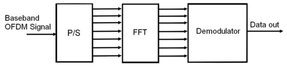
In the Fig 2.1 we can see the basic structure of an OFDM transmitter.

Fig 2.1 – Basic OFDM transmitter.

The signal is then submitted to a serial to parallel conversion (S/P), where

the serial bitstream is converted into several parallel bitstreams to be divided

among the individual carriers. After that the signal is transmitted through the

channel, being the channel the route that the signal goes through from the

ceiver to the transmitter. When the frequency signals reach the receiver, the

re-ceiver must perform the synchronization (both in time and frequency), channel

Estimation, demodulation and decoding. At the receiver the data processing is

converted using a parallel to serial conversion (P/S) and a fast Fourier

transfor-mation (FFT) block is firstly used to transfer the received time-domain signal into

frequency-domain. Ideally, the output of the FFT block should be identical to the

transmitted symbols before the IFFT block. Assuming that the information about

the channel is know, the symbols will be demodulated and estimated based on

In Fig 2.2 we can see the basic structure of a OFDM receiver.

Fig 2.2 – Basic OFDM Receiver.

When there is more than one transmission path between the transmitter and

the receiver, or the received signal is the sum of many versions of the transmitted

signal with different delays and attenuations, it causes ISI effect. To reduce this

effect, two methods are generally used in the OFDM scheme: parallel data

trans-mission and cyclic prefix. Usually the length of the cyclic prefix is longer than the

length of the channel’s impulse response. The basic idea is to replicate part of the

OFDM time-domain block from the back to the front to create a guard period.

The duration of the guard period 𝑇_𝑔 should be longer than the worst-case delay

spread of the channel. The structure of cyclic prefix is illustrated in Figure 2.3,

[18].

Fig 2.3 – Signal with Cyclic prefix

OFDM signals are known to have substantial envelope fluctuations, which

MIMO-OFDM schemes [19]. In the last years, several techniques to combat the large

en-velope fluctuations of OFDM signals have been proposed [20]. The simplest ones

based on nonlinear clipping operations [21], [22].

2.2

–

MIMO System

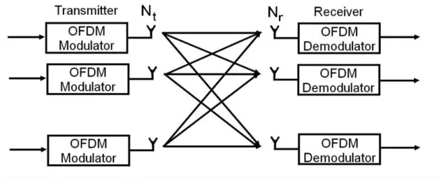
MIMO is a technology that uses multiple antennas at the transmitter and

at the receiver to transmit and receive signals. In the Fig. 2.4 it is shown the basic

concept of a MIMO system.

Fig 2.4 – MIMO structure.

In a MIMO system, the data [𝑥₁, 𝑥₂, … . 𝑥_𝑁] is transmitted with N

transmit-ting antenna arrays. The receiver is composed by M (M≥N) antenna arrays. Let

𝑟𝑗( j= 1, 2,…, M ) represents the signal received by the 𝑗𝑡ℎ antenna. The signals received

at the receiver can be represented as:

𝑟1 = ℎ11 𝑥1+ ℎ12𝑥2+ ⋯ + ℎ1𝑁𝑥𝑁 , (2.1)

𝑟2 = ℎ21 𝑥1+ ℎ22𝑥2+ ⋯ + ℎ2𝑁𝑥𝑁 , (2.2)

where h ij is a weight coefficient that represents the impact of the 𝑗𝑡ℎ transmitting

signal 𝑥_𝑗on the 𝑗𝑡ℎ receiver signal strength. We define a frequency channel matrix

H as:

H=(

ℎ11

ℎ21

ℎ12

ℎ22 ⋯ ℎ

1𝑁

ℎ2𝑁

⋮ ⋮ ⋱ ⋮

ℎ𝑀1 hM2 ⋯ ℎ𝑀𝑁

). (2.4)

Therefore, in MIMO system, the transmitted signals {𝑥_𝑖} can be recovered

by estimating the channel matrix H and the receiving signal vector R.

MIMO systems can provide two types of gains: diversity gain and spatial

multiplexing gain. It is known that there is a fundamental tradeoff between these

two gains: higher spatial multiplexing gain comes at the price of sacrificing

di-versity [23]. Didi-versity is used in MIMO to combat channel fading. Since in MIMO

each pair of transmitting and receiving antennas provides a signal path from the

transmitter to the receiver and each path carries the same information

simultane-ously, the signal achieved in the receive antenna is more reliable and the fading

can be effectively decreased. If the path gains between individual transmit–

re-ceive antenna pairs fade independently, in this case multiple parallel spatial

channels are created. By transmitting independent information streams in

paral-lel through the spatial channels, the data rate can be increased. This effect is also

called spatial multiplexing [24].

The benefit of using diversity is a higher SNR and a lower error probability

and the benefit of using multiplexing is that it allows a higher rate. Diversity

re-quires that the same information is sent by all the antennas, and multiplexing

requires independent information to be sent by each antenna. Because of that

order to get the benefits required from the use of one or the other accordingly to

the location requirements.

2.3

–

MIMO-OFDM System

MIMO OFDM is a technology that combines MIMO and OFDM together

to transmit data in wireless communications in order to deal with frequency

se-lective channel effect. The OFDM signal on each subcarrier can overcome

nar-rowband fading, therefore, OFDM can transform frequency-selective fading

channels into parallel flat ones. Then by combining MIMO and OFDM

technol-ogy together, MIMO algorithms can be applied in broadband transmission [25].

A MIMO OFDM system transmits data modulated by OFDM from

multi-ple antennas simultaneously. At the receiver, after OFDM demodulation, the

sig-nal is recovered by decoding each one of the sub-channels from all the transmit

antennas [26]. MIMO-OFDM takes advantage of the multipath properties of

en-vironments using base station antennas without NLOS. By using MIMO and

OFDM, a higher throughput can be achieved.

Fig 2.5- Basic structure MIMO-OFDM

In Figure 2.5, the basic structure of MIMO OFDM is shown. In this figure,

MIMO system, finally, the signals are recovered by the OFDM demodulator.

Therefore, MIMO OFDM achieves spectral efficiency, increased throughput and

ISI can thus be prevented.

2.4

–

Diversity combining techniques

Nowadays, the most popular transmit diversity techniques in use are

Selec-tion diversity, space time coding (Alamouti scheme) and beamforming

tech-niques. It will be also explored the usage of Maximal-Ratio combining (MRC) in

which the estimations of different channels are coherently combined to recover

the transmit signals.

2.4.1 – Selection Diversity

In MIMO systems, selection diversity selects the branch providing the

larg-est magnitude of log-likelihood ratio (LLR). The LLR for Binary Phase-shift

key-ing (BPSK) signals in fading channels is found to be proportional to the product

of the fading amplitude and the matched filter output after phase compensation.

Channel state includes statistics information such as fading amplitudes,

phases and delay. In selection diversity technique, none of these channel

infor-mation parameters are required. Selection diversity uses one receiver antenna

which greatly reduces the complexity of the wireless systems. Here, the receiver

simply looks at the outputs from each fading channel and selects the one with

the highest SNR. In this case, the strongest signal is picked up and other signals

that have undergone deep fades are unlikely to be picked by the receiver, which

can avoid the deep fading effect. Therefore, the more the channels are, the more

accurate the recovered signal would be. There is also no need for any addition of

the fading channel outputs, which further decreases the complexity. Since

Selec-tion diversity does not require any knowledge of the phases, it is usually used in

non-coherent or differential coherent modulation schemes. The signals from the

system and finally received by the receive antenna. The structure for this type of

diversity can be seen in Fig. 2.6

Fig.2.6 – Basic structure of transmit selection diversity.

2.4.2 – Alamouti Scheme

Alamouti scheme is an orthogonal transformation scheme that gives the

second order transmission diversity, which is applied to the receiver that can

greatly reduce the complexity of the receiver. The Alamouti scheme also assumes

that the channel is invariant in the two transmission intervals.

2.4.3 – Alamouti Scheme with two transmitter antennas one receiver

an-tenna

The MIMO Alamouti code is a simple space time block code (STBC), where

the different replicas sent for exploiting diversity are generated by a space-time

encoder which encodes a single stream through space using all the transmit

an-tennas and through time by sending each symbol at different times.

The Alamouti STBC scheme uses two transmit antennas and Nr receive antennas

At the transmitter of the Alamouti scheme, the two signals 𝑥₁ , 𝑥₂ are

trans-mitted at the same time from the two transmitting antennas. In this case, 𝑥₁, 𝑥₂

are baseband complex symbols carrying the information.

The time and transmit sequence are shown as the following:

Symbols x 1 and x 2 are sent with the first beam at time t, while -𝑋₂*and 𝑋₁* (*

stands for complex conjugate) are transmitted through the second antenna at

time t+T, where T is the symbol duration[27]. Where we assume that the rows of

each coding scheme represent a different time instant, while in this case, the first

and second rows represent the transmission at the first and second time instant

respectively.

The channel model is

ℎ1 = ℎ1(𝑡+𝑇)= 𝐻1 = 𝑎1𝑒𝑗𝜃1 (2.7)

ℎ2 = ℎ2(𝑡+𝑇)= 𝐻2 = 𝑎2𝑒𝑗𝜃2

At the receiver of the Alamouti scheme, the signals are respectively

re-ceived at times t and t+T, where

𝑅₁ = 𝐻₁𝑋₁+ 𝐻₂𝑋₂+ 𝑁₁ (2.8)

𝑅2 = −𝐻1𝑋2∗+ 𝐻2𝑋1∗+ 𝑁2

Time Antenna1 Antenna2

T 𝑋1 𝑋2

Here 𝑟₁, 𝑟₂are the received signals and 𝑛₁, 𝑛₂are the complex random

vari-ables representing the noise and interference. The received symbols are then

combined and processed by the decoder. The receivers obtain the signals 𝑠₁ , 𝑠₂

through the following matrix after computing the estimates of the complex

chan-nel gains, that is,

𝑆₁ = 𝐻₁∗𝑅₁+ 𝐻₂𝑅₂∗ (2.9)

𝑆2 = 𝐻2∗𝑅1− 𝐻1𝑅2∗

2.4.4 – Alamouti Scheme two transmitter antennas two receiver antenna

When it is used an Alamouti scheme with two transmitter antennas and one

receiver antenna its possible to have a diversity of 2. When a Alamouti scheme

with two transmitter antennas and two receiver antennas is used, it is possible to

have a diversity of 4. In this case, the transmission sequence has minor change

from the two transmitters and one receiver Alamouti scheme [28].

The transmitting signals at the transmitting antennas are the following:

Time Antenna1 Antenna2

T 𝑋1 𝑋2

t+T -𝑋₂* 𝑋₁*

where symbols 𝑋₁and 𝑋₂are sent with the first beam at time t, while -𝑋₂*and 𝑋₁*

are transmitted through the second beam at time t+T, where T is the symbol

du-ration.

The receiving signals at the receiving antennas are shown in the following

Time Antenna1 Antenna2

T 𝑅1 𝑅2

t+T 𝑅3 𝑅4

There are four communication channels between the two transmitter

anten-nas and two receiver antenanten-nas, which are defined as 𝐻₁, 𝐻₂. 𝐻₃, 𝐻₄ respectively.

The relationship between the receiving and transmitting signals can be

repre-sented as:

𝑅1 = 𝐻1𝑋1+ 𝐻2𝑋2+ 𝑁1

𝑅2 = −𝐻1𝑋2∗+ 𝐻2𝑋1∗+ 𝑁2 (2.10)

𝑅3 = 𝐻3𝑋1+ 𝐻4𝑋2+ 𝑁3

𝑅4 = −𝐻3𝑋2∗+ 𝐻4𝑋1∗+ 𝑁4,

where 𝑋₁, 𝑋₂represent the transmitted signals 𝑅, 𝑅₂, 𝑅₃, 𝑅₄are the received

sig-nals and 𝑁₁, 𝑁₂, 𝑁₃, 𝑁₄ are complex random variables representing the noise and

interference. The receivers then obtain the signals 𝑆₁, 𝑆₂ after computing the

es-timates of the complex channel gains, that is,

𝑆1 = 𝐻1∗𝑅1+ 𝐻2𝑅2∗+ 𝐻3∗𝑅3 + 𝐻4𝑅4 , (2.11)

𝑆2 = 𝐻2∗𝑅1− 𝐻1𝑅2∗+ 𝐻4∗𝑅3− 𝐻3𝑅4∗ .

In this case, the results of this scheme are equivalent to those obtained by

the 4-branch MRC scheme [29].

2.4.5 – Beamforming technique

In beamforming transmission scheme, usually the CSI should be known at

the transmitter, so we use the known channel information to code the

simpli-fied. For example, in a one-transmitter–two-receiver Beamforming scheme,

as-sume that the transmitted signal is X, the first channel as 𝐻₁and the second

chan-nel as 𝐻₂where

𝐻₁ = 𝑎₁𝑒𝑗𝜃1 (2.12)

𝐻2 = 𝑎2𝑒𝑗𝜃2.

The signal transmitted by the first transmitting antenna is 𝑋𝐻₁∗ and the signal

transmitted by the second transmitting antenna is, X𝐻₂∗.

After going through the channels, signals that are received by the receivers could

be represented as:

𝑅1 = 𝑋 𝐻1∗𝐻1+ 𝑁1 = 𝑎12𝑥 + 𝑁1, (2.13)

𝑅2 = 𝑋 𝐻2∗𝐻2+ 𝑁2 = 𝑎22𝑥 + 𝑁2,

where 𝑅_1,, 𝑅₂are the received signals and 𝑁₁, 𝑁₂, are complex random variables

representing the noise and interference.

The combining scheme for two-branch Beamforming is:

𝑆′ _{= 𝑅}

1+ 𝑅2 = 𝑎12𝑥 + 𝑁1+ 𝑎22𝑋 + 𝑁2 (2.14)

= (𝑎12+ 𝑎22)𝑥 + 𝑁1+ 𝑁2.

After equalizing the coefficient (𝑎₁2+ 𝑎₂2), we can get the final signal after

decision making. The benefits of MIMO beamforming is that the power gain and

array gain get increased and the co-channel inter-cell interference is reduced.

Also the diversity gain get increased, because Beamforming can combat the

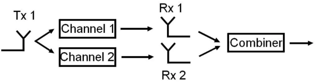
2.4.6 – Maximal-ratio combining (MRC)

The MRC is a diversity technique over fading channels. While it is slightly

more complex than Selection Diversity, the performance is especially good in the

case of independent fading channels.

MRC selects all the branches and gets the average square value of each

branch to decrease Rayleigh fading. The basic structure of MRC scheme is

illus-trated in Figure 2.7.

Fig 2.7 Basic structure of Maximal-ratio Receiver Combining.

Let us first consider a one-transmitter-two-receiver MRC model. At a given

time, a signal 𝑥 is sent from the transmitter. The channels between the transmit

antenna and the receive antennas are denoted by 𝐻₁and 𝐻₂ given by

𝐻₁ = 𝑎₁𝑒𝑗𝜃1, (2.15)

𝐻2 = 𝑎2𝑒𝑗𝜃2.

Considering the noise and interference added at the two receivers, the

re-sulting received signals could be written as:

𝑅1 = 𝐻1𝑋 + 𝑁1, (2.16)

𝑅1 = 𝐻2𝑋 + 𝑁2,

where 𝑅₁, 𝑅₂are the received signals and 𝑁₁, 𝑁₂ are complex random variables

After the combiner we have:

𝑆′_{= 𝐻}

1∗𝑅1+ 𝐻2∗ 𝑅2 = 𝐻1∗ (𝐻1𝑋 + 𝑁1) + 𝐻2∗(𝐻2𝑋 + 𝑁2) (2.17)

Then after equalizing the coefficient 𝑎₁2 + 𝑎₂2, we can get the final signal after

Capacity of the System

In this chapter we describe the results of capacity for several systems, that

were the result of a developed software program, that simulates the SISO and

MIMO system. First we describe the capacity for a linear SISO system. Second

the capacity for a nonlinear SISO system. Third the capacity for a linear MIMO

system, and finally the capacity for a nonlinear MIMO system. The channel is

frequency-selective and based on a cluster ray model where the antennas have a

correlation factor. In the case of MIMO-OFDM it will be considered a scenario

with T transmitter antennas and R receiver antennas. The total number of

multi-path components is L = G X B, where G is the number of clusters of B rays. The

channel is represented by the R X T matrix given by

ℎ(𝑡) = ∑𝐿−1𝑙=0𝜷(𝑙)𝛿(𝑡 − 𝜏𝑙) , (3.1)

where 𝜏_𝑙 and 𝛽(𝑙) are the delay and the channel matrix associated with the 𝑙𝑡ℎ tap.

The channel matrix for the 𝑙𝑡ℎ path is,

𝛽(𝑙) ₌

[

𝛽1,1(𝑙) 𝛽1,2(𝑙) … 𝛽1,𝑡(𝑙)

𝛽_2,1(𝑙) 𝛽_2,2(𝑙) … 𝛽_2,𝑡(𝑙) ⋮

𝛽_𝑟,1(𝑙) …… …⋱ ⋮ 𝛽_𝑟,𝑡(𝑙)_]

,

where 𝛽_𝑟,𝑡(𝑙) is the fading coefficient between the 𝑟𝑡ℎreceive antenna and the 𝑡𝑡ℎ

transmit antenna for the 𝑙𝑡ℎ tap. Each OFDM block is formed by P = min(T; R)

streams with 𝑁_𝑡 subcarriers and is represented by the 𝑃 𝑋 𝑁_𝑡 matrix

𝑆 = [ 𝑆(0)

𝑆(1)

⋮ 𝑆(𝑃)

] = [𝑆(0) 𝑆(1) … 𝑆(𝑝)]. (3.3)

This matrix can be decomposed along its lines or its columns. On one

hand, we use the 1 𝑥 𝑁_𝑇 matrix 𝑆(𝑝) = [𝑆₁(𝑝) _𝑆2(𝑝) _{… 𝑆𝑁𝑇}𝑃 ] to represent the set

of data symbols associated to the 𝑝𝑡ℎ stream. On the other hand, we use the P x 1

matrix 𝑆 = [𝑆(𝑘)₁ 𝑆(𝑘)₂ … 𝑆(𝑘)𝑝]𝑇 to define the set of data symbols

associ-ated to the 𝑘𝑡ℎ subcarrier. Regarding the composition of each OFDM signal, only

N of the 𝑁_𝑇 subcarriers are effectively used to transmit data. The other 𝑁_𝐺 =

N(M-1) subcarriers are left idle so as to obtain an oversampling operation by a factor

of M. Therefore, 𝑆(𝑘)_𝑝 = ±𝜎_𝑆± 𝑗𝜎_𝑆 and E[|𝑆(𝑘)_𝑝|2]= 2σ𝜎_𝑆2 for k ∈N and 𝑆(𝑘)_𝑝 =

0.

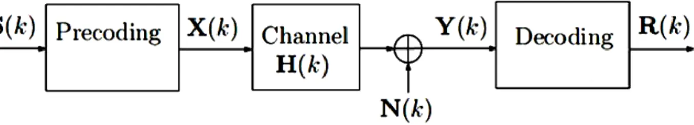
The signal will then be submitted to a precoding technique. It will be

con-sidered the SVD technique for the precoding and decoding operation because of

its properties, and because we are interested in the system capacity [29][30]. Of

course, such precoding and decoding operation requires the perfect channel

knowledge at the receiver and transmitter.

This means that there will be a precoding operation at the transmitter and

level. With the SVD, the channel matrix associated to the kth subcarrier is

decom-posed as

𝐻(𝑘) = 𝑈(𝑘)𝛬(𝑘)𝑉𝐻_{(𝑘), (3.4)}

where U(k) and 𝑉𝐻(k) are the matrices used for the decoding and precoding pro-cesses, respectively. Λ(k) = ([ 𝛬(𝑘)₁ 𝛬(𝑘)₂ … 𝛬(𝑘)_𝑝] is a diagonal matrix

com-posed by the P non-zero singular values of H(k), with 𝛬(𝑘)₁ > 𝛬(𝑘)₂> … > 𝛬(𝑘)_𝑝.

The precoded version of S(k) is X(k), where

𝑋(𝑘) = 𝑉(𝑘)𝑆(𝑘), (3.5)

with V(k) denoting the precoding matrix with dimensions T x P . The

time-do-main version of X(k) is obtained through an inverse discrete Fourier transform

(IDFT), i.e.,

𝑥(𝑡) _{= [𝑥}

1(𝑡) 𝑥2(𝑡)… 𝑥𝑁𝑇

(𝑡) _{]. (3.6)}

After the precoding operation, the resulting signal is submitted to a

non-linear power amplifier (PA), and the output is

𝑦(𝑡) = 𝑓(𝑥(𝑡)). (3.7)

The nonlinear PA is modeled as a bandpass memoryless nonlinearity,

characterized by the amplitude modulation/amplitude modulation (AM/AM)

and amplitude modulation/phase modulation (AM/PM) conversion functions

A(.) and θ(.), respectively. For a given input 𝑥_𝑛(𝑡) = |𝑥_𝑛(𝑡)| exp (𝑗𝑎𝑟𝑔(𝑥_𝑛(𝑡))), the PA

yields

Without loss of generality, we considered the specific model of a solid

state power amplifier (SSPA) [31]. This amplifier has negligible AM/PM

charac-teristic and AM/AM characcharac-teristic given by

𝐴 (|𝑥𝑛(𝑡)|) = |𝑥𝑛 (𝑡)_|

√1+|𝑥𝑛(𝑡)|_𝑆𝑀2𝑞

2𝑞 , (3.9)

where 𝑆_𝑀 denotes the saturation level (naturally, the performance will be

condi-tioned by the normalized saturation level 𝑆_𝑀/𝜎_𝑥, where 𝜎_𝑥 is the variance of the

real and imaginary parts of the precoded OFDM signal) and q defines the

sharp-ness of the transition between the linear and nonlinear regions. When q =∞ the

amplifier turns into an ideal envelope clipping with clipping level 𝑆_𝑀 .

Due to the Gaussian nature of the precoded OFDM signal at the

nonlin-ear input, one can take advantage of the Bussgang’s theorem [32]. This allows

us to decompose a nonlinearly distorted Gaussian signal into two uncorrelated

components: a useful component that is a scaled version of the input signal and

a term that concentrates the nonlinear distortion [33]. Therefore, we may write

the nonlinearly distorted signal at the output of the 𝑡𝑡ℎPA as

𝑦(𝑡) _{= 𝑓(𝑥}(𝑡)_{) = 𝛼}(𝑡)_𝑥(𝑡)_{+ 𝑑}(𝑡)_{, (3.10)}

where 𝑑 = [𝑑₁(𝑡) _𝑑2(𝑡) _{… 𝑑3}(𝑡)] is the set of nonlinear distortion terms of the

𝑡𝑡ℎ _{branch and 𝛼}(𝑡) _{is the scale factor associated to the 𝑡}𝑡ℎ _{branch that can be}

ob-tained as

𝛼(𝑡) ₌ 𝐸[𝑥𝑛(𝑡)𝑦𝑛∗(𝑡)] 𝐸[|𝑥_𝑛(𝑡)|2_] =

𝐸[𝑥𝑛(𝑡)𝑓∗(𝑥𝑛(𝑡))]

2𝜎_𝑛2 . (3.11)

In fact, since it is assumed that the nonlinear characteristics of the power

precoded signals is the same for all branches, the scale factor of (3.12) is

inde-pendent of t and 𝛼(𝑡)= 𝛼 ∀ 𝑡. The discrete Fourier transform (DFT) of (3.10) yields the frequency-domain version of the signal to be transmitted 𝑌(𝑡) =

𝐷𝐹𝑇([𝑦₁(𝑡) 𝑦₂(𝑡) … 𝑦_𝑁(𝑡)_𝑇]). Once again, from the Bussgang’s theorem, we can

sepa-rate into two uncorrelated components, leading to

𝑌(𝑡)_{= 𝛼𝑋}(𝑡)_{+ 𝐷}(𝑡)_{, (3.12)}

where 𝐷(𝑡)= 𝐷𝐹𝑇([𝑑₁(𝑡) 𝑑₂(𝑡) … 𝑑_𝑁(𝑡)_𝑇]) represents the nonlinear distortion terms

along the 𝑡𝑡ℎ branch. Under these conditions, the nonlinearly distorted signal for

the kth subcarrier is

𝑌(𝑡) = 𝛼𝑋(𝑘) + 𝐷(𝑘). (3.13)

The nonlinearly amplified signals are transmitted through the

frequency-selec-tive channel represented in (3.1). Since the 𝑘𝑡ℎ channel is represented by H(k),

the received signal is

𝑊(𝑘) = 𝐻(𝑘)𝑌(𝑘) + 𝑁(𝑘), (3.14)

where 𝑁(𝑘) = [𝑁(𝑘)₁ 𝑁(𝑘)₃ … 𝑁(𝑘)_𝑅]𝑇represents the noise components

asso-ciated to the 𝑘𝑡ℎ subcarrier. The power of the noise is 𝐸 = [|𝑁(𝑘)_𝑟2] = 2𝜎_𝑁2, with

𝜎𝑁2 defined according to the desired SNR. Our SNR definition accounts for the

impact of the nonlinear distortion effects and is dependent on the fraction of

power wasted in the nonlinear distortion term. This “degradation” is measured

by the ratio

𝜂 = 𝑃𝑢

𝑃𝑢+𝑃𝑑 , (3.15)

where 𝑃_𝑢 = |𝛼|2 𝐸 [ |𝑥_𝑛(𝑡)|2] and 𝑃_𝑑 = 𝐸 [|𝑦_𝑛(𝑡)|2] - 𝑃_𝑢 represent the useful power

and the power associated to the nonlinear distortion component, respectively.

Therefore,

𝑆𝑁𝑅 = 𝐸[|𝛼𝑆(𝑘)𝑟|2] 𝜂𝐸[|𝑁(𝑘)𝑟|2] =

𝐸[|𝛼𝑆(𝑘)𝑟|2]

By using (3.13) and (3.14), we have

𝑊(𝑘) = 𝐻(𝑘)(𝛼𝑋(𝑘) + 𝐷(𝑘)) + 𝑁(𝑘). (3.17)

To complete the SVD process, the received signal W(k) decoded by the matrix 𝑈𝐻(𝑘), leading to 𝑅(𝑘) = [𝑅(𝑘)₁ 𝑅(𝑘)₂ … 𝑅(𝑘)_𝑝 ]𝑇. The decoded signal can be written as

𝑅(𝑘) = 𝑈𝐻_{(𝑘)𝑊(𝑘) = 𝑈}𝐻_{(𝑘)(𝐻(𝑘)𝑌(𝑘) + 𝑁(𝑘))}

= 𝑈𝐻_{(𝑈(𝑘)𝛬(𝑘)𝑉}𝐻_{(𝑘)(𝛼(𝑘)𝑋(𝑘) + 𝐷(𝑘)) + 𝑁(𝑘)}

= 𝛼𝛬(𝑘)𝑆(𝑘) + 𝛬(𝑘)𝑉𝐻_{(𝑘)𝐷(𝑘) + 𝑈}𝐻_{𝑁(𝑘). (3.18)}

From (3.18), one can note that the SVD decomposition allows the

trans-mission of P decoupled flat-fading OFDM streams that can be analyzed

sepa-rately. The singular value 𝑘𝑡ℎ represents the flat-fading coefficient associated the

pth stream of kth subcarrier.

3.1 Capacity of a linear SISO system

A linear SISO system is a system with only one transmitter antenna and a

single receiver antenna, that as the addiction of AWGN to the signal. In Fig 3.1 it

is shown the system.

Fig 3.1 Linear SISO System

The signal S is submitted to a precoding operation that will result in the

signal X, then it will be transmitted across the channel. When X reaches the

result in the channel Y. After that, the signal will be submitted to the decoding

operation, resulting finally in the signal R. The resulting capacity for such

ap-proximation can be directly taken from the Shannon theorem seen in (1.5).

In this case it is considered the use of a SVD technique as the precoding

and decoding operation to deal with the effects of the channel. It is considered

that there is a perfect channel estimation in both the receiver and transmitter, that

will allow the use of the SDV technique on the channel, in order to deal with the

effects that the channel will introduce to the signal. In Fig. 3.2 it is show the

scheme for such a system.

Fig 3.2 Linear SISO System with SVD

Considering a system with one transmitter antenna and one receiver

an-tenna, H being the channel and the SVD decomposition of the channel being

𝐻 = 𝑈𝜆𝑉𝐻_{, (3.19)}

where 𝑉𝐻 is the precoding matrix and U is the decoding matrix, the signal at the

input of the channel is

𝑋 = 𝑉𝑆. (3.20)

The received signal is

𝑌 = 𝐻𝑋 + 𝑁= 𝐻𝑉𝑆 + 𝑁

= 𝑈𝜆𝑉𝑉𝐻_{𝑆 + 𝑁 = 𝑈𝜆𝑆 + 𝑁. (3.21)}

The decoding signal is obtained by multiplying (3.21) by 𝑈𝐻 resulting in

𝑅 = 𝑈𝐻_{𝑌 = 𝑈}𝐻_{𝑈𝜆𝑆 + 𝑈}𝐻_𝑁

In this case, the calculation of the capacity respects the Shannon theorem

on capacity, allowing the easy calculation of the capacity of the channel.

Throughout the simulation of results, we proceeded to the calculation on

the capacity of the SISO system using SVD. It was used the approximation

equa-tion

𝐶 = log2(1 + 𝑆𝑁𝑅). (3.23)

For this approximation, it is considered that the SNR can be described by

𝑆𝑁𝑅 = |𝜆|_{𝐸[|𝑁′|}2𝐸[|𝑆|_2]2] . (3.24)

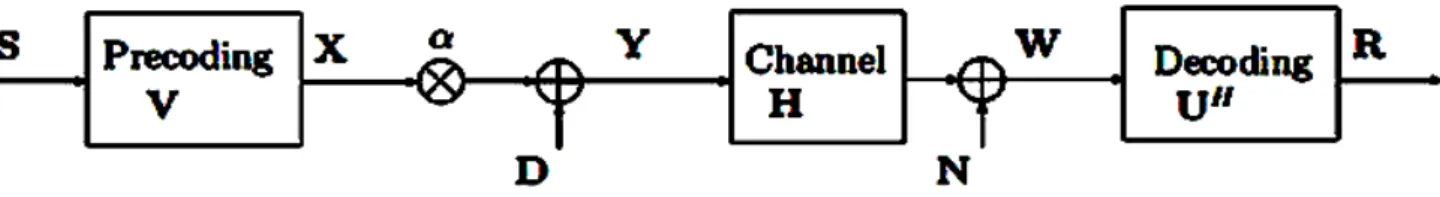
3.2 Capacity of a nonlinear SISO system

A nonlinear SISO system it is a system that has the addition of a nonlinear

distortion added to the signal. It will be considered that the nonlinear effect can

be compared to a Solid State Power Amplifiers, SSPA amplifier, since the

multi-plication for α and the addiction of interference can simulate the non linear

ef-fects to with the signal will be subjected. In fig 3.3 it is show the nonlinear SISO

system.

In Fig. 3.3 it is possible to see the representation of the SISO system. S

rep-resents the symbol to be transmitted, X the result after the precoding, α is the

scalar amplification of a SSPA, D is the distortion introduced by the SSPA, Y is

the transmitted signal that will go through the channel H, N represents the

AWGN, W is the signal before the decoding operation and R, the final received

signal. Since we are considering a SISO system for a single symbol, all the factors

Fig 3.3 – Non Linear SISO system.

For a nonlinear SISO -OFDM transmission in ideal AWGN channels, the

received signal for the 𝑘𝑡ℎ subcarrier is [16], [34]

𝑌(𝑘) = 𝛼𝑆(𝑘) + 𝐷(𝑘) + 𝑁(𝑘), (3.25)

where S(k), D(k) and N(k) are the transmitted signal, the distortion signal and

the noise signal for the 𝑘𝑡ℎ subcarrier. Therefore, the corresponding signal to

in-terference and noise ratio (SINR) for the kth subcarrier is [35]

𝑆𝐼𝑁𝑅𝑆𝐼𝑆𝑂_{(𝑘) =} |𝛼|2𝐸[|𝑆(𝑘)|2]

𝐸[|𝐷(𝑘)|2_{]+𝐸[|𝑁(𝑘)|}2_] . (3.26)

In this case we considered the use of SSPA, to recreate the nonlinear effects

that the signal is submitted. The nonlinearity can be viewed as the multiplication

of the signal by a scalar α and the addiction of distortion represented in the figure

as D.

So the system using a SVD precoding and decoding can be represented as seen

in fig. 3.4.

With H being the channel and the SVD decomposition of the channel

be-ing

𝐻 = 𝑈𝜆𝑉𝐻_{, (3.27)}

𝑉𝐻 _{is the precoding matrix and U is the decoding matrix, the signal at the input} of the channel is

𝑋 = 𝑉𝑆. (3.28)

The signal after the nonlinear effect will be

𝑌 = 𝛼𝑋 + 𝐷. (3.29)

then, the resulting signal Y will be submitted to the channel H and will suffer the addiction of noise resulting in the received signal W:

𝑊 = 𝐻𝑌 + 𝑁 = 𝛼𝐻𝑋 + 𝐻𝐷 + 𝑁

= 𝛼𝐻𝑉𝑆 + 𝐻𝐷 + 𝑁 = 𝛼𝑈𝜆𝑉𝐻_{𝑉𝑆 + 𝑈𝜆𝑉}𝐻_{𝐷 + 𝑁}

= 𝛼𝑈𝜆𝑆 + 𝑈𝜆𝑉𝐻_{𝐷 + 𝑁. (3.30)}

The decoding signal is obtained by multiplying (3.29) by 𝑈𝐻 resulting in

𝑅 = 𝑈𝐻_{𝑊 = 𝑈}𝐻_{𝛼𝑈𝜆𝑆 + 𝑈}𝐻_𝑈𝜆𝑉𝐻_{𝐷 + 𝑈}𝐻_𝑁

= 𝛼𝜆𝑆 + 𝜆𝑉𝐻_{𝐷 + 𝑈}𝐻_{𝑁 = 𝛼𝜆𝑆 + 𝐷′ + 𝑁′. (3.31)} Therefore, the corresponding signal to interference and noise ratio (SINR) for the kth subcarrier is (3.26)

For large SNR values, (i.e. 𝐸[|𝑁(𝑘)|2 → 0 ) the SINR reduces to the signal to in-terference ratio (SIR) and, for the 𝑘𝑡ℎ subcarrier, we may write

𝑆𝐼𝑅𝑆𝐼𝑆𝑂_{(𝑘) ≃}|𝛼|2𝐸[|𝑆(𝑘)|2]

3.3 Capacity of a linear MIMO System

The analysis of the nonlinear MIMO system is in many ways equal do the

approximations made to the linear SISO system. The channel will suffer the same

decomposition but now we will be dealing with a large number of antennas, both

in the receiver as in the transmitter.

The capacity associated to the 𝑘𝑡ℎsubcarrier of the 𝑝𝑡ℎ stream is

𝐶𝐻_(𝑘)

𝑝 = log2(1 + 𝑆𝑁𝑅𝐻(𝑘)𝑝) . (3.33)

The total capacity associated to the 𝑘𝑡ℎsubcarrier is

𝐶𝐻_{(𝑘) = ∑ 𝐶}𝐻_(𝑘)

𝑝 𝑃

𝑝=1 . (3.34)

And the average capacity of the block for a given channel realization is

𝐶𝐻′(𝑘) ₌ 1

𝑁 ∑𝑁𝑘=1𝐶𝐻(𝑘). (3.35)

The fig 3.5 shows the evolution of the channel capacity associated to linear

massive MIMO-OFDM systems considering frequency selective channels with L

= 12, where G = 3, B = 4 and = 0.5. OFDM signals have N = 128 and M = 4. It can

be observed in the figure that the capacity increases with the SNR. When the

number of transmitter antennas is doubled, we can observe that the capacity also

increases, the difference in capacity when it is observed T=8 and T= 16, it is not

linear, as the SNR increases, the gain in capacity that is possible by duplicating

the number of antennas, goes from around 5 bps/Hz in the case of SNR= -10dB’s,

up to around 20 bps/Hz in the case of SNR=30dB’s. When we double the number

of antennas from 16 to 32, the difference in capacity between T=32 and T= 16 goes

Fig 3.5- Evolution of capacity of the linear MIMO-OFDM for different

values of T.

3.4 Capacity of a nonlinear MIMO System

The analysis of the nonlinear MIMO system is in many ways equal do the

approximations made to the nonlinear SISO system. The channel will suffer the

same decomposition, but now we will be dealing a large number of antennas,

both in the receiver as in the transmitter. We start to obtain the SINR the 𝑘𝑡ℎ

sub-carrier of the 𝑝𝑡ℎ stream considering a given channel realization. In order to do

that, we write the received signal for the kth subcarrier of the 𝑝𝑡ℎ stream as (see

(3.18))

Being 𝛼𝛬(𝑘)_𝑝𝑆(𝑘)_𝑝 the signal component and 𝛬(𝑘)_𝑝𝐷′(𝑘)_𝑝+ 𝑁′(𝑘)_𝑝 the noise

and distortion component. Under these conditions, the SINR for the kth

subcar-rier of the 𝑝𝑡ℎstream is

𝑆𝐼𝑁𝑅𝐻_(𝑘)

𝑝 = |𝛼| 2_|𝛬(𝑘)

𝑝|2𝐸[|𝑆(𝑘)𝑝|2]

|𝛬(𝑘)𝑝|2𝐸[|𝐷′(𝑘)𝑝|2]+𝐸[|𝑁′(𝑘)𝑝|2] . (3.37)

However, when T > R, it can be shown that [36][37]

𝐸 [|𝐷′_(𝑘)

𝑝|2] = 𝐸[| ∑ 𝑉𝐻(𝑘)𝑐,𝑡 𝑇

𝑡=1

𝐷(𝑘)𝑡|2]

≈𝑅_𝑇𝐸[|𝐷(𝑘)|2_{]. (3.38)}

In fact, (3.37) reveals that there is a linear relation between the spectral

dis-tribution of the nonlinear distortion term in each one of the P streams and the

nonlinear distortion term associated to a nonlinear SISO-OFDM system. This

re-lation is approximately T/R, which shows that the robustness to nonlinear

distor-tion effects increases with T (considering a fixed number of streams). Fig. 3.6

shows the spectral distribution of the nonlinear distortion term concerning the

first stream (p=1) i.e. 𝐸[|𝐷′(𝑘)₁|2for R = 8and different values of T as well as the

Fig 3.6 – Evolution of 𝐸[|𝐷(𝑘)|2] and 𝐸[|𝐷′(𝑘)₁|2] for different values of T

and R=8.

The OFDM signals have N = 256 and M = 4 and the SSPA is parameterized

by q = 1 and 𝑆_𝜎𝑀

𝑥 = 0.5. From this figure it can be noted that for that the case of

Nonlinear Massive MIMO with R = T = 8, it possible to have 𝐸[|𝐷′(𝑘)₁|2 ≈

𝐸[|𝐷(𝑘)|2_{, that meaning we have the same value of 𝐸[|𝐷(𝑘)|}2_{] that is expected}

for the Nonlinear SISO -OFDM, T=R = 1 and in contrast, the spectral distribution

of the nonlinear distortion term decreases by a factor of T/R = 1/2 when T = 16

and T/R = 1/4 when T = 32, which confirms that the distortion level can be greatly

reduced when T≫ R. Therefore, (3.37) can be rewritten as

𝑆𝐼𝑁𝑅𝐻_(𝑘)

𝑝= |𝛼|

2_{|𝛬(𝑘)𝑝|}2_{𝐸[|𝑆(𝑘)𝑝|}2_]

The capacity associated to the 𝑘𝑡ℎsubcarrier of the 𝑝𝑡ℎ stream is

𝐶𝐻_(𝑘)

𝑝 = log2(1 + 𝑆𝐼𝑁𝑅𝐻(𝑘)𝑝)) . (3.40)

The total capacity associated to the 𝑘𝑡ℎsubcarrier is

𝐶𝐻_{(𝑘) = ∑ 𝐶}𝐻_(𝑘)

𝑝 𝑃

𝑝=1 , (3.41)

and the average capacity of the block for a given channel realization is

𝐶𝐻_{′(𝑘) =}1

𝑁 ∑𝑁𝑘=1𝐶𝐻(𝑘). (3.42)

Therefore, the total capacity can be obtained by averaging (3.42) over the

channel realizations (i.e. over H),

𝐶 = 𝐸𝐻[𝐶𝐻′] . (3.43)

Fig. 3.7 shows the evolution of the channel capacity associated to nonlinear

mas-sive MIMO-OFDM systems considering frequency selective channels with L = 12,

where G = 3, B = 4 and 𝑆_𝜎𝑀

𝑥= 0.5. OFDM signals have N = 128 and M = 4. We

con-sidered massive MIMO-OFDM systems with R = 8 and different values of T. The

Fig. 3.7 - Evolution of the capacity for nonlinear channel for 𝑆_𝜎𝑀

𝑥 = 0,5, q = 1, R = 8

and different values of T.

From figure 3.7 it can be noted that as the number of transmit antennas

increases, not only the linear channel capacity increases (as expected), but also

the capacity associated to the nonlinear massive MIMO-OFDM increases. In fact,

the “floor level” of the nonlinear channel capacity increases due to the fact that

the PSD associated to the nonlinear distortion term decreases with T for a fixed

number of streams. For low SNR, it should be pointed out that the linear and

nonlinear channel capacities are not exactly equal. The difference between them

is related with the fraction of power wasted in the nonlinear distortion

Fig. 3.8 shows the evolution of η considering different saturation levels and

dif-ferent values of q. As expected, the stronger the nonlinearity the larger the

deg-radation, since the distortion component is higher (moreover, there is more

power wasted in its transmission, i.e., decreases). Meaning that to counterbalance

this effect, with will need to use more power in the signal transmission, in order

to increase the SINR. When an ideal envelope clipping is considered (i.e., for

q=+∞), the degradation with 𝑆_𝑀/𝜎_𝑥= 0.5 can be 0.5 dB.

Fig. 3.9 shows the evolution of the linear and nonlinear channel capacities for R

= 8 and T = 32 considering an SSPA with q = 1 and different saturation levels.

From the figure it can be noted that the larger the saturation level, the better the

capacity. In fact, the capacity floors increase substantially with 𝑆_𝑀/𝜎_𝑥. [38]

Fig 3.9- Evolution of the channel capacity for R = 8, T = 32, different saturation levels and q = 1.

It is possible to determine that for different saturation levels the capacity of the massive MIMO system also changes. With the increase of 𝑆_𝜎𝑀

𝑥 the capacity of the

system also increases, and for the considered SNR interval the difference can be as high as 7 bps/Hz for SNR=30dB’s and 20dB’s.

By analysis of the several simulations it can be show that the evolution of capacity does not have a linear behavior in terms of gain of bps/Hz. But it can be clarified that as expected the bigger the number of transmission antennas, the higher it will be the capacity, and that there is an increase of the capacity according to the 𝑆𝑀