MIMO Array Capacity Optimization
Using a Genetic Algorithm
Manuel O. Binelo, André L. F. de Almeida,
Member, IEEE
, and F. Rodrigo P. Cavalcanti,
Member, IEEE
Abstract—This paper discusses the design of multiple-input–multiple-output (MIMO) antenna systems and proposes a genetic algorithm to obtain the position and orientation of each MIMO array antenna that maximizes the ergodic capacity for a given propagation scenario. One challenging task in the MIMO system design is to accommodate the multiple antennas in the mobile device without compromising the system capacity, due to spatial and electrical constraints. Based on an interface between the antenna model and the propagation channel model, the ergodic capacity is considered as the objective function of the MIMO array optimization. Simulation results corroborate the importance of polarization and antenna pattern diversities for MIMO in small terminals. Our results also show that the electromagnetic coupling effect can be exploited by the optimizer to decrease signal correlation and increase MIMO capacity. A comparison among a uniform linear array (ULA), a uniform circular array (UCA), and a genetic algorithm (GA)-optimized array is also carried out, showing that the topology given by the optimizer is superior to that of the standard ULA and UCA for the considered propagation channel.
Index Terms—Array optimization, capacity, genetic algorithm (GA), multiple-input–multiple-output (MIMO).
I. INTRODUCTION
M
ULTIPLE-input–multiple-output (MIMO) systems have been an important research topic due to their capability of providing a significant increase in channel capacity pro-portional to the number of transmit and/or receive antennas. This is generally achieved by exploiting spatial diversity at the transmit and receive branches [1], [2]. When considering realistic antenna models, the channel capacity will depend on three main variables, namely, the transmit antenna array configuration, the receive antenna array configuration, and the environment configuration, i.e., the distribution of the channel scatterers [3].Manuscript received November 29, 2010; revised March 16, 2011 and May 18, 2011; accepted May 21, 2011. Date of publication June 2, 2011; date of current version July 18, 2011. This work was supported in part by the Innovation Center, Ericsson Telecomunicações S.A., Brazil, by Sony Ericsson Mobile Communications do Brasil Ltda, and by Conselho Nacional de Desenvolvimento Científico e Tecnológico under Grant 312845/2009-0. The review of this paper was coordinated by Prof. E. Bonek.
M. O. Binelo is with the Wireless Telecom Research Group, Federal Univer-sity of Ceará, 60455-760 Fortaleza-CE, Brazil, and also with the UniverUniver-sity of Cruz Alta, 98025-810 Cruz Alta-RS, Brazil (e-mail: manuel@gtel.ufc.br).
A. L. F. de Almeida and F. R. P. Cavalcanti are with the Wireless Telecom Research Group, Federal University of Ceará, 60455-760 Fortaleza-CE, Brazil (e-mail: andre@gtel.ufc.br; rodrigo@gtel.ufc.br).
Color versions of one or more of the figures in this paper are available online at http://ieeexplore.ieee.org.
Digital Object Identifier 10.1109/TVT.2011.2158460
Multiplexing and diversity gains in MIMO systems can be obtained, for instance, by resorting not only to spatial diversity but to polarization diversity as well. Whereas spatial diversity can be achieved by ensuring enough antenna separation, polar-ization diversity can be achieved by exploiting different antenna orientations in the array configuration [4]. In cellular systems, a reasonable degree of spatial diversity can be obtained at the base station. However, at the mobile terminal, this situation is completely different since a good separation of the antennas ensuring spatial diversity is not always possible. Moreover, electromagnetic coupling between terminal antennas is a prac-tical problem that affects system performance. Therefore, under these constraints, optimizing the antenna placement at the mo-bile terminal to yield a satisfactory performance is a challenging problem [5], [6].
The work in [7] shows some important aspects about im-plementation of MIMO transceivers in small terminals. In [8], planar inverted-F antenna (PIFA) compact arrays are compared with dipole arrays with the same antenna separation. That work states that PIFA antennas are an ideal candidate for compact array designs due to the low interference between antennas caused by the proximity to the ground plane. Although find-ing the globally optimal antenna set was not in the scope of [8], the work allows one to conclude about the importance of empirical inference from the designer. The dipoles were uniform linear arrays (ULAs), whereas the PIFAs had a 180◦ difference in orientation between the two elements. The PIFA arrays outperformed the dipoles. The said paper attributes this result to the nearly omnidirectional pattern of the PIFA, but it does not justify the position and orientation of the used PIFA antennas and does not investigate the influence of the orientation.
In [9], the relationship between MIMO capacity and array configuration is investigated for different outdoor propagation scenarios. The work concludes that, for a small angular spread of 8◦, the best separation of antenna array elements would be four wavelengths to approximate the uncorrelated channel performance, whereas for 68◦, the optimum distance is the typical 1/2 wavelength. It is also noted in that work that, with higher angle spreads, the system was less sensitive to array orientation changes. In general, these works corroborate the relevance of the propagation environment characteristics in the design of the MIMO array.
Another very important MIMO diversity technique is true polarization diversity (TPD). In TPD, instead of typical al-ternated 0◦ and 90◦ polarization, we can use any angle to change polarization. This is particularly useful for small mobile terminals that have small space for exploring spatial diversity.
The study in [4] shows that TPD can significantly improve MIMO capacity. However, now, the designer has to deal not only with antenna positioning in the array but also with an-tenna orientation, bringing more complexity to the transceiver design. Not only the orientation of individual array elements is important, but the orientation of the hole array also has an important impact on MIMO capacity, particularly for small angle spreads, typically in outdoor environments, according to [10]. In [11], a model for antenna correlation using arbitrary antenna orientation is used, and the work also shows that using different orientations for the antennas increases MIMO capac-ity. In [12], the challenges of antenna configurations in small mobile terminals are discussed. The work uses a measurement system to evaluate antenna configurations. The conclusions of the work are that small changes in antenna configuration can cause drastic changes in capacity and that the directive proper-ties of the antennas and propagation channel cause important fluctuations on performance.
In [13], the question is whether UCAs are better for MIMO capacity than ULAs. It turns out that ULAs are better for some direction-of-arrival (DOA) configurations whereas UCAs have a more stable behavior. A similar analysis is made in [14]. However, the question on the MIMO transceiver design is much wider. Which array arrangement is better for a given propagation scenario or for a given set of scenarios? Which array configuration, from a MIMO capacity viewpoint, is more stable?
Reviewing these works, we can see that the possibilities for the MIMO system designer are endless, and just studying reference cases might not be enough to find a solid solution. Using optimization tools that can take all these possibilities into account may yield more robust MIMO designs.
Suppose that the designer knows the antenna model and the number of antenna elements to be used in a mobile termi-nal. Given an available space at the terminal for placing the antennas, a pertinent question is now in order. What are the best antenna configurations to be used in a given propagation environment? To answer this question, a possible road to take is to make use of experimental results or intuition to find a probable good antenna configuration for a certain propagation scenario and then use simulation or prototype measurements to see if the design fulfills the project requisites.
The second approach is to use an optimization method for finding an optimal (or suboptimal) solution to the antenna array configuration problem and then check if this solution is satisfactory. In this case, we jump from a computer-aided design paradigm to a computer design one. This approach has become increasingly common, as shown in [15].
Genetic algorithm (GA)-based optimization has been used with success in various engineering problems. In [16], a GA is used to optimize antenna arrays used for channel charac-terization, i.e., determination of multipath DOAs. The system starts with big regular 2-D or 3-D array of antennas (more than 20 antennas), and then, the algorithm changes individual antenna position and orientation by trying to find the array that minimizes the parameter estimation error. Although the obtained antenna positioning patterns may seem random and sometimes not intelligible for the designer, they offer better
precision in terms of channel characterization than usually regular (or uniformly spaced) patterns.
In [17], the authors resort to GA-based optimization to find channel parameters such as multipath attenuations and delays. In [18], a GA is used for blind channel estimation. The study reports that the GA method can offer better channel estimation accuracy than traditional methods. A similar approach was also proposed in [19]. Recently, a GA has been used to find good antenna element positions in sparse MIMO radar arrays [20] by minimizing the sidelobes of the radar pattern. Another recent work [21] used a GA to find the optimal distribution of a 3× 3 MIMO system for an indoor propagation channel. An inter-esting aspect of that work is the inclusion of electromagnetic coupling in the model. However, the work does not show either which distributions were found or how the distributions change according to different multipath channel parameters.
The work in [22] defends the idea of using nature-inspired methods for MIMO antenna design, but the works mentioned in there deal with the problem of antenna geometry definition and not antenna array topology for different propagation envi-ronments. In [23], a method of moments (MOM) is proposed to optimize MIMO antenna position and orientation. The op-timization is done by minimizing antenna cross correlation by considering an independent and identically distributed (i.i.d.) propagation scenario. Although antenna cross correlation de-grades capacity, we cannot say that the configuration that minimizes antenna correlation is the same configuration that maximizes MIMO capacity in non-i.i.d. propagation scenarios. A similar approach is used in [24]. The work in [25] solves the problem of MIMO PIFA placement for an i.i.d. channel, also minimizing antenna cross correlation, but using the infinitesi-mal dipole method and invasive weed optimization, which is another nature-inspired method.
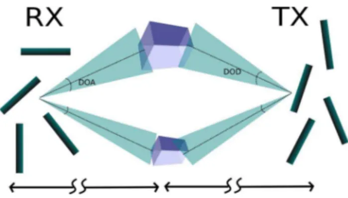
Fig. 1. Geometric channel model used in simulations.
ergodic channel capacity as the fitness function of the GA. Section IV presents simulation results and results discussion. Finally, in Section V, we draw conclusions.
II. CHANNELMODEL
In Fig. 1, the channel geometric model used to generate the plane waves and to interface it to the antenna arrays is illustrated. We assume that the distance between antenna arrays and the scattering clusters is much higher than the distance between the array elements. In this case, we can assume that the DOA and the direction of departure (DOD) of a given plane wave are the same for all the antenna elements of the array. Each cluster is modeled by a finite set of plane waves and has a main DOA/DOD, both in azimuth and elevation. Angle spread and polarization spread within a cluster follow a Gaussian distribution.
The channel double-directional impulse response, which is associated with the DOA pair (φRx, θRx) and the DOD pair
(φTx, θTx), is given by the contribution of a finite number of
dominant multipath components [28], i.e.,
A(φRx, θRx, φTx, θTx) =
L
l=1
Al(φRx,l, θRx,l, φTx,l, θTx,l)
(1)
whereLis the number of arriving paths, andφandθdenote the azimuth and elevation angles, respectively. The contribution of each pathAlcan be expanded as follows:
Al(φRx, θRx, φTx, θTx) =Wlejφl ×δ(φRx−φRx,l)δ(θRx−θRx,l)
×δ(φTx−φTx,l)δ(θTx−θTx,l) (2)
where φl=j2πfc, and Wl is the polarimetric transmission
matrix, which is defined as
Wl=
γHH γVH
γHV γVV
. (3)
The(m, n)th entryhm,nof MIMO channel matrixH(M ×
N)can be expressed in terms of the directional channel impulse
response according to the following expression [28]:
hmn= L
l=1
gTTx(φTx,n,l, θTx,n,l,rTx,n) ×Al(φRx,l, θRx,l, φTx,l, θTx,l) ×gRx(φRx,m,l, θRx,m,l,rRx,m) ×exp (j[k(φRx,l, θRx,l)·xRx,m])
×exp (j[k(φTx,l, θTx,l)·xTx,n]) (4)
where gRx is the antenna pattern response to the direction
(φRx,m,l, θRx,m,l), andgTxis the antenna pattern response to
the direction(φTx,m,l, θTx,m,l)at the transmitter. The response
of the antenna considers the impact of mutual electromagnetic coupling of nearby antennas. We calculate this effect by inte-grating the numerical electromagnetics code (NEC) in our sim-ulation. The (2×1) vectorgRx is the product of the complex
scalar gain gRx(phase and amplitude) of the receiver antenna
and the unitary (2×1) polarization vectorpRx composed of
vertical and horizontal responses, i.e.,
gRx(φRx,n,l, θRx,n,l,rRx,n)=gRx(φRx,n,l, θRx,n,l,rRx,n)pRx.
(5)
Similarly, for transmitter antenna pattern response gTx, we
have
gTx(φTx,n,l, θTx,n,l,rTx,n)=gTx(φTx,n,l, θTx,n,l,rTx,n)pTx.
(6)
VectorrRx,mis the antenna orientation,kis the wave vector,
xRx is the relative position of the mth receiver antenna, and
xTxis the relative position of thenth transmitting antenna. The
inner product of vector wave k (arriving or departing wave) with an antenna position (transmitter or receiver) is defined by
k(φ, θ)·x=2π
λ(xcosθcosφ+ycosθsinφ+zsinθsinφ). (7)
Fig. 2 shows the interface between the antenna and the propa-gation environment, which is used to build the effective MIMO channel response. Note that (4) is an entry of the effective
MIMO radio channel, which includes the effect of antenna responses in the channel impulse response. As we will see later, the position and orientation of each receive antenna, which are defined by vectorsxRx andrRx, respectively, are variables to
be optimized by the proposed optimization algorithm. Vector rRx is composed of elementsα,β, andγ, which represent the
rotations around the x-, y-, and z-axes, respectively. In this paper, we limit ourselves to the optimization of the receive array parameters. The joint optimization of the receive and transmit array parametersxTxandrTxis left to future work.
A. Electromagnetic Coupling
Fig. 2. Antenna–propagation environment interface.
available and well-established code, which is integrated to our channel model. We use the NEC [29], which is a public domain software. The version we chose to work with is NEC2C, which is a C language implementation of the NEC2 Fortran original code. The NEC uses the MOM to solve the electromagnetic field problem. One of its main qualities is the low computational cost of the solutions, since MOM codes are much faster than, e.g., finite-element-method-based codes.
The mutual coupling of the antennas affect the far-field response of the antennas in two ways. First, it changes the mag-nitude of the response, modifying the directivity of the antenna. Second, it perturbs the phase response of the antenna. Fig. 3 shows both effects in a dipole antenna under the influence of mutual coupling with a nearby dipole antenna. It is worth noting that the effect of mutual coupling will not always degrade MIMO capacity. Depending on the considered channel model and on the antenna configuration, it may well increase capacity by decorrelating the signal (true MIMO gain) or by increasing the directive gain toward a cluster direction. The work in [10] explains how electromagnetic coupling can decrease antenna correlation by means of pattern diversity. Since in small termi-nals it is not possible to use spatial separation of antennas to achieve diversity, it is important to consider mutual coupling as a possible source of pattern diversity and not just a downside in MIMO antenna design.
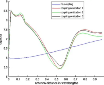
Fig. 4 shows the capacity of a 2 ×2 MIMO system as a function of antenna separation for a channel with one cluster. When the antennas are very close, there is a strong gain in capacity for the system with antenna mutual coupling. This is caused not only by the signal decorrelation effect but also by a directive gain toward the cluster. The drop in capacity for a distance of λ/2 and its raise at 0.8λ are caused by correlation and decorrelation effects of mutual coupling. Our results corroborate the works in [5] and [6], where the same pattern of the raise in correlation (drop in capacity) atλ/2and the drop in correlation (raise in capacity) at0.2λand0.8λis found.
Fig. 3. Effect of mutual coupling in the far field of a dipole antenna.
Fig. 4. Effect of mutual coupling on MIMO capacity.
III. GENETICALGORITHMOPTIMIZATION
A GA works by analogy to genetic inheritance and differen-tiation that occurs in biology that permits a species to fit itself to the environment in an adaptation process. We can think about the channel characteristics as the environment and the antenna array as the biologic species that needs to fit in the environment (the channel). The fitness of the antennas to the environment can be measured by the ergodic capacity. As a bird can develop a beak more adapted to a specific kind of seed, by analogy, an antenna array could develop characteristics better suited for a specific channel or kind of channel.
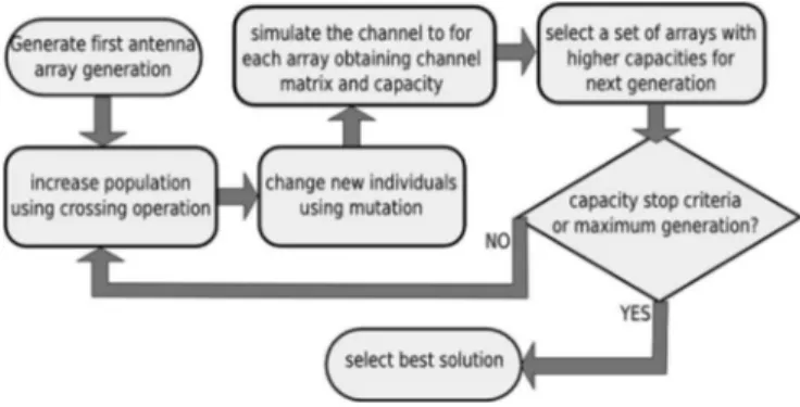
Fig. 5. Fluxogram of the employed GA.
genetic code is the channel array model stored in the computer memory. A population, or generation, is a collection of antenna arrays. The genes that define an array are the antenna type, position, and orientation. We start with a random generation, where each antenna has a position and an orientation assigned to it by a random variable with a uniform distribution, within the limits of the desired volume space for the antennas. The number of individuals in the generation is increased by crossing and mutation. The crossing operation is the reproduction of new individuals that inherit part of the characteristics from one individual and other part from other individuals, e.g., the parents. Which characteristic will come from each parent is decided by an aleatory factor. The mutation operation is an aleatory small change in the genes.
The next step is to select the individuals better suited to the environment using the fitness function and then repeat the reproduction step with this selected group. The reproduction and selection steps are repeated until an optimization criterion is met or a certain number of generations are met. Our fitness function is defined by the channel ergodic capacity, as will be detailed later.
We can see the GA as a method that explores a search space. The randomness of mutation makes the optimizer explore dif-ferent regions escaping from local maxima, whereas the fitness function gives a direction to the search. One advantage of the proposed GA is its low sensibility for initial conditions when compared with traditional numerical methods. A very useful aspect of the GA is that, as a searching algorithm, it is not limited to numerical field operations and can use any operation that can be expressed in the algorithm. One example of this feature would be the search for the best kind of antenna for a given scenario or even to merge different antennas into the same solution. A limitation of this method is that it can stop in a local maximum, and in some cases, it is not possible to know if the solution is local or global, or if the algorithm is capable or not of leaving the local maxima. Fig. 5 shows a general diagram of the GA optimization method that is applied to our problem.
A. Population and Reproduction
The antenna is represented in the system by the tuple
(kind,position,orientation). The kind is an integer token that identifies the antenna far-field pattern. In this paper, we consider ideal half-wave dipoles, although more than one kind of antenna could be used. Position vector x= [x, y, z]T and orientation
vectorr= [α, β, γ]T (yaw, pitch, roll). A collection of antennas [a1, a2, . . . , aM]defines an array. An array is one individual in
the population. The GA needs a finite set into which to search; thus, the position and orientation need to be both limited and quantized. The degrees of freedom of the position are limited by a limited volume defined prior to the simulation. The available volume is generally a practical constraint of the antenna array design in small terminals. The quantization is naturally imposed by the computer quantization of the floating-point numbers. Defining the antenna geometry by a collection of 3-D pointsS, its radiation pattern is rotated by the following transformation:
S′= (c1 c2 c3)S (8) where
c1=
⎛
⎝
cosγ cosβ cosα−sinγ sinα −sin γcosβ cosα−cosγ sinα
sinβ cosα
⎞
⎠ (9)
c2=
⎛
⎝
cosγ cosβ sin α+ sin γcosα
−sin γcosβ sinα+ cosγcosα sin β sinα
⎞
⎠ (10)
c3=
⎛
⎝
−cosγ sinβ sin γsinβ
cosβ ⎞
⎠. (11)
The genetic code of each individual in the collection is formed by the antennas’ tuples. The reproduction is done by combining portions of the deoxyribonucleic acid from two parents. A new array is derived by choosing antennas from two ancestor arrays. A pseudorandom function is used to choose from which parent each antenna will be copied for the new individual in the population. After the reproduction, a small pseudorandom change is made in each antenna parameter. Such a change defines the mutation procedure. It is worth noting that the amount and extent of the mutation have a strong impact on the algorithm performance. Small changes can make the algorithm converge faster, but it is more prone to get stuck in a local maximum, whereas stronger changes make it leave the local maximum for better maxima but makes the system less stable. Therefore, a tradeoff between convergence speed and stability exists, as usual in numerical optimization methods.
Another parameter to take into account is the size of the offspring in each generation. A small offspring provides faster computation and less memory usage, at the expense of more iterations necessary to solve the problem. Fig. 6 shows the reproduction and mutation operations, whereα1toα6denote a random displacement.
B. Fitness Function
Fig. 6. Crossing and mutation procedure.
Fig. 7. Fitness function used in the GA.
obtained by the crossing and mutation operations. The output of the function has to be some value attached to each individual, making it possible to classify it. In our case, that value corre-sponds to the ergodic channel capacity (in bits per channel use), which is given by [30]
C= 1
Nq Nq
q=1
log2det
IN r+
SNR N t HqH
H q
(12)
whereNq is the number of realizations to compute the
expec-tation statistics, andHq represents theqth channel realization.
Note that, according to (4), each entryhmn ofHq (M ×N)
depends on relative antenna positionsxRx,1,...,M and antenna
far-field patterns according to their orientationsrRx,1,...,M at a
given channel realization. Recall that only the receive antennas are the object of the present investigation. The antennas at the transmitter (i.e., the base station for the downlink) are supposed to have fewer placement constraints and are not optimized here. Therefore, the objective function of the GA is to solve the following problem:
arg max xRx,1,...,M,rRx,1,...,M
C(xRx,1,...,M,rRx,1,...,M). (13)
The diagram given in Fig. 7 illustrates the fitness function. Indexirefers to theith array configuration in the generation population, whereas indexkrefers to thekth generation in the simulation. These two pieces of information generate a set of plane waves that are stored and remain constant during all the simulations. This is important because each generation is not a leap in time. The succession of generations is time related in nature but has no relation to the time variation of the radio channel. The collection of plane waves has two dimensions. We refer tow as the wave index and q as the realization index. A number of wave realizations are first generated and stored and further used to compute the statistics of ergodic channel
Fig. 8. Capsule collision detection.
capacity. The same random realizations have to be applied for each individual of the generation; otherwise, a noise would be added to the solution. It is interesting to note that this architecture makes it possible to use any channel environment definition model that delivers a set of plane waves as the output. Even real site channel characterization measurements might be used.
The NEC is integrated to our optimization software in the fitness function, as shown in Fig. 7. For each iteration, and for each array in the population of possible solutions, the input files that define the geometry and electric characteristics of the antennas are created. Then, the NEC is invoked, and its solver calculates the far-field results of the antennas considering the mutual coupling effect. The NEC then writes the far-field results to its output files. Our software then reads the NEC output files and proceeds with the channel simulation for the fitness function.
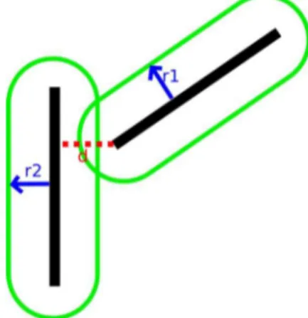
One problem initially faced during the simulations was the fact that, when two antennas had an intersection, the NEC would see a short circuit between the antennas, generating incorrect far-field results. The problem was solved by applying a collision test during the phase of reproduction of antennas. Every antenna wire was protected by a capsule. The system measures the minimum distance between antennas’ wires; if this distance is greater than the sum or than capsule radios r1 andr2, the antennas are considered to be in collision, and
the array is dropped from the population. This idea is shown in Fig. 8.
IV. SIMULATIONRESULTS
Here, a set of computer simulation results is presented for some propagation scenarios and system configurations. We aim at investigating the link between the GA-optimized antennas’ positions and orientations to the propagation environment in question. We also evaluate the theoretical channel capacity obtained by optimizing the antenna array configurations using the proposed GA algorithm.
A. One Cluster, 3×3 MIMO
Fig. 9. Evolved 3×3 MIMO configuration. One cluster with a fixed main direction. SNR= 20dB. Volume= (2λ)3.
Fig. 10. Histogram for the evolved 3×3 MIMO configuration. One cluster with a fixed main direction. SNR= 20dB. Volume= (2λ)3
.
two wavelengths. The propagation channel is characterized by a single scattering cluster with high angle spread and total polarization diversity. Since there is a large space for the system to exploit, any solution with antenna separation greater than λ/2 and polarization diversity will be a good solution. We made 20 simulations, and all results presented a pattern similar to that of Fig. 9. The lines in the figure present a sampling of the DOAs, and the line color represents its polarization, ranging from fully horizontal to fully vertical. Fig. 10 shows the histogram of the ergodic capacity of the initial random antenna positions and orientation, as well as the ergodic capac-ities obtained after optimization. The initial ergodic capacity had a mean of 9.48 bits/s/Hz with a standard deviation of 1.01 bits/s/Hz. The GA improved it to a mean of 14.14 bits/s/Hz with a standard deviation of 0.43 bit/s/Hz.
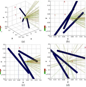
Fig. 11. First evolved 3×3 MIMO configuration. One cluster with a fixed main direction. SNR= 20dB. Volume= (0.2λ)3
.
Fig. 12. Second evolved 3×3 MIMO configuration. One cluster with a fixed main direction. SNR= 20dB. Volume= (0.2λ)3
.
B. One Cluster, 3×3 MIMO, Small Volume
Fig. 13. Evolved 3×3 MIMO configuration. One cluster with a uniformly distributed main direction. SNR= 20dB. Volume= (0.2λ)3.
capacity of mean 11.89 bits/s/Hz and standard deviation of 0.33 bit/s/Hz. The initial conditions of the antennas had a mean of 6.76 bits/s/Hz and a standard deviation of 0.92 bit/s/Hz.
Fig. 13 shows the simulation results for a 3 × 3 MIMO system with a search space limited to0.23
λ. It also considers one cluster, but this time, the cluster main direction is not fixed but uniformly distributed around the space. The cluster has the same angle spread of other simulations but is not plotted in the figure due to its main direction distribution. In this case, all 20 simulations had shown results similar to that of Fig. 11. Since the available space is too small to achieve signal diversity through antenna spacing, the optimizer made use of two strategies, i.e., orthogonal polarizations and orthogonal pat-terns. According to Fig. 11, antenna 3 is orthogonally polarized to antennas 1 and 2. Antennas 1 and 2 are placed in parallel. The electromagnetic coupling effect makes antennas 1 and 2 get directional gains in opposite directions. Fig. 14 shows how the optimizer made use of polarization and pattern diversity, ex-ploiting the electromagnetic mutual coupling effect, to produce MIMO diversity.
Fig. 15 shows the histogram for all 20 simulations for one cluster with a fixed main direction. Fig. 16 shows the histogram for one cluster with a uniformly distributed main direction. Fig. 17 shows the evolution of the solutions for this last sim-ulation scenario. We can see the ability of the system to escape from a local maximum.
C. Array Topology Comparison
In [13], an ULA is compared with an UCA. The work in [31] shows the impact of DOA over correlation for the ULA, and the correlation degrades MIMO capacity. The capacity is calculated for one cluster for different DOAs using a 4 × 4 MIMO
Fig. 14. Resulting antenna pattern for the evolved 3×3 MIMO configuration. One cluster with a fixed main direction. SNR= 20dB. Volume= (0.2λ)3
.
Fig. 15. Histogram for the evolved 3×3 MIMO configuration. One cluster with a fixed main direction. SNR= 20dB. Volume= (0.2λ)3
.
Fig. 16. Histogram for the evolved 3×3 MIMO configuration. One clus-ter with a uniformly distributed main direction. SNR= 20 dB. Volume= (0.2λ)3.
Fig. 17. A 3×3 MIMO array evolution in a small volume.
Fig. 18. Schematic of the ULA and UCA.
Fig. 19. Array topology resulted from GA optimization.
Fig. 20. Performance comparison of ULA, UCA, and GA array topologies.
Fig. 21. Histogram for the evolved 4×4 MIMO configuration. Uniform cluster main direction distribution. SNR= 20dB. Volume= (0.2λ)3.
could not escape from a local optimum. This behavior indicates that the proposed algorithm can be further improved to avoid such local optima.
V. CONCLUSION
The proposed GA-based optimization algorithm for antenna array positioning has proved to be successful in finding good MIMO antenna schemes for a given propagation scenario. Some solutions found by the GA optimizer were very subtle, and a human designer would have difficulties in trying to iden-tify the best location and orientation for the antennas according to the specified propagation environment. The comparison of the ULA, the UCA, and the array evolved by our method shows that it is a much more efficient engineering method than the intuitive and trial-and-error approach.
The results so far have shown that pattern and polarization diversities play an important (if not the most important) role in MIMO capacity when there is little space available to position the antennas. One important aspect of the proposed method is its generality, as it can be adapted to be used with different antenna and propagation models.
As a perspective of this work, we should consider the use of different types of antennas: preferably practical mobile terminal antennas.
REFERENCES
[1] G. J. Foschini and M. J. Gans, “On limits of wireless communications in a fading environment when using multiple antennas,”Wireless Person. Commun., vol. 6, no. 3, pp. 311–335, Mar. 1998.
[2] I. E. Telatar, “Capacity of multiantenna Gaussian channels,”Eur. Trans. Telecommun., vol. 10, no. 6, pp. 585–595, Nov./Dec. 1999.
[3] A. Glazunov, M. Gustafsson, A. Molisch, F. Tufvesson, and G. Kristens-son, “Spherical vector wave expansion of Gaussian electromagnetic fields for antenna–channel interaction analysis,”IEEE Trans. Antennas Propag., vol. 57, no. 7, pp. 2055–2067, Jul. 2009.
[4] J. Valenzuela-Valdes and D. Sanchez-Hernandez, “Increasing handset performance using true polarization diversity,” inProc. 69th IEEE VTC Spring, Apr. 26–29, 2009, pp. 1–4.
[5] B. Lindmark, “Capacity of a 2×2 MIMO antenna system with mutual coupling losses,” inProc. Int. Symp. IEEE Antennas Propag. Soc., 2004, vol. 2, pp. 1720–1723.
[6] X. Liu and M. E. Bialkowski, “Effect of antenna mutual coupling on MIMO channel estimation and capacity,”Int. J. Antennas Propag., vol. 2010, no. 8, pp. 1452–1463, 2010.
[7] D. Manteuffel, “MIMO antenna design challenges,” in Proc. LAPC, Loughborough, U.K., Nov. 16–17, 2009, pp. 50–56.
[8] D. Browne, M. Manteghi, M. Fitz, and Y. Rahmat-Samii, “Experiments with compact antenna arrays for MIMO radio communications,”IEEE Trans. Antennas Propag., vol. 54, no. 11, pp. 3239–3250, Nov. 2006. [9] P. Lusina and F. Kohandani, “Analysis of MIMO channel capacity
depen-dence on antenna geometry and environmental parameters,” inProc. 68th IEEE VTC, Sep. 21–24, 2008, pp. 1–5.
[10] L. Xin and N. Zai-ping, “Effect of array orientation on capacity of MIMO wireless channels,” inProc. 7th Int. Conf. ICSP, Aug. 31–Sep., 4, 2004, vol. 3, pp. 1870–1872.
[11] L. Wang and H. G. Wang, “An analytical three dimensional correlation model for array with antennas having arbitrarily oriented directions,” in
Proc. APMC, Dec. 16–20, 2008, pp. 1–4.
[12] P. Vainikainen, M. Mustonen, M. Kyro, T. Laitinen, C. Icheln, J. Villanen, and P. Suvikunnas, “Recent development of MIMO antennas and their evaluation for small mobile terminals,” inProc. 17th Int. Conf. MIKON, May 2008, pp. 1–10.
[13] X. Liu and M. Bialkowski, “Effective degree of freedom and channel ca-pacity of a MIMO system employing circular and linear array antennas,” inProc. 5th Int. Conf. WiCom, Sep. 24–26, 2009, pp. 1–4.
[14] L. Jian-gang, L. Ying-hua, H. Peng-fei, and L. Peng, “Evaluation of capacity of indoor MIMO channel with different antennas array,” inProc. IEEE Int Symp. MAPE, Aug. 8–12, 2005, vol. 1, pp. 204–207.
[15] X. Chen, K. Huang, and X.-B. Xu, “Automated design of a three-dimensional fishbone antenna using parallel genetic algorithm and NEC,”
IEEE Antennas Wireless Propag. Lett., vol. 4, no. 1, pp. 425–428, 2005. [16] P. Karamalis, A. Kanatas, and P. Constantinou, “A genetic algorithm
applied for optimization of antenna arrays used in mobile radio channel characterization devices,”IEEE Trans. Instrum. Meas., vol. 58, no. 8, pp. 2475–2487, Aug. 2009.
[17] A. Ebrahimi and A. Rahimian, “Estimation of channel parameters in a multipath environment via optimizing highly oscillatory error functions using a genetic algorithm,” inProc. 15th Int. Conf. SoftCOM, Sep. 27–29, 2007, pp. 1–5.
[18] L. Hua, Z. Wei, Z. Qing-hua, W. Hua-kui, and Z. Zhao-xia, “Blind estima-tion of MIMO channels using genetic algorithm,” inProc. 5th Int. Conf. ICNC, Aug. 14–16, 2009, vol. 4, pp. 163–167.
[19] S. Chen and Y. Wu, “Genetic algorithm optimisation for maximum likeli-hood joint channel and data estimation,” inProc. IEEE Int. Conf. Acoust., Speech Signal Process., May 12–15, 1998, vol. 2, pp. 1157–1160. [20] Z. Zhang, Y. Zhao, and J. Huang, “Array optimization for MIMO radar
by genetic algorithms,” inProc. 2nd Int. Congr. CISP, Oct. 17–19, 2009, pp. 1–4.
[21] A. Farkasvolgyi, R. Dady, and L. Nagy, “Channel capacity maximization in MIMO antenna system by genetic algorithm,” inProc. 3rd EuCAP, Mar. 23–27, 2009, pp. 1119–1122.
[22] Y. Rahmat-Samii, “Modern antenna designs using nature inspired opti-mization techniques: Let Darwin and the bees help designing your multi band MIMO antennas,” inProc. IEEE Radio Wirel. Symp., Jan. 2007, pp. 463–466.
[23] M. Mohajer and S. Safavi-Naeini, “MIMO antenna optimization using method of moments analysis,” inProc. IEEE iWAT, Mar. 2009, pp. 1–4. [24] M. Mohajer, G. Rafi, and S. Safavi-Naeini, “MIMO antenna design
and optimization for mobile applications,” in Proc. IEEE APSURSI, Jun. 2009, pp. 1–4.
[25] S. Karimkashi, A. Kishk, and D. Kajfez, “MIMO antenna system opti-mization for mobile applications using equivalent infinitesimal dipoles,” inProc. IEEE APSURSI, Jul. 2010, pp. 1–4.
[26] M. Binelo, A. de Almeida, J. Medbo, H. Asplund, and F. Cavalcanti, “MIMO channel characterization and capacity evaluation in an outdoor environment,” inProc. IEEE 72nd VTC-Fall, 2010, pp. 1–5.
[27] L. Ximenes and A. de Almeida, “Capacity evaluation of MIMO antenna systems using spherical harmonics expansion,” inProc. IEEE 72nd VTC-Fall, 2010, pp. 1–5.
[28] N. Costa and S. Haykin,Multiple-Input Multiple-Output Channel Models, Theory and Practice. New York: Wiley, 2010.
[29] D. Nitch and A. Fourie, “A redesign of NEC2 using the object-oriented paradigm,” inProc. Int. Symp. AP-S. Dig., Jun. 1994, vol. 2, pp. 1150– 1153.
[30] A. Goldsmith,Wireless Communications. New York: Cambridge Univ. Press, 2005.
[31] J.-A. Tsai, R. Buehrer, and B. Woerner, “The impact of AOA energy distribution on the spatial fading correlation of linear antenna array,” in
Proc. IEEE 55th VTC Spring, 2002, vol. 2, pp. 933–937.
Manuel O. Binelo received the B.Sc. degree in computing science from the University of Cruz Alta, (UNICRUZ), Cruz Alta, Brazil, in 2004 and the M.Sc. degree in mathematical modeling from the Regional University of Northwest of Rio Grande do Sul State, Ijuí, Brazil, in 2007. He is currently working toward the Ph.D. degree in teleinformatics engineering with the Federal University of Ceará, Fortaleza, Brazil.
André L. F. de Almeida(M’08) received the B.Sc. and M.Sc. degrees in electrical engineering from the Federal University of Ceará, Fortaleza, Brazil, in 2001 and 2003, respectively, and the double Ph.D. degree in sciences and teleinformatics engineering from the University of Nice-Sophia Antipolis, Nice, France, and the Federal University of Ceará in 2007. In 2002, he was a Visiting Researcher with Ericsson Research, Stockholm, Sweden. He was a Postdoctoral Fellow with the Computer Science, Sig-nals and Systems Laboratory, Centre National de la Recherche Scientifique, University of Nice-Sophia Antipolis, from January to December 2008. He is currently an Assistant Professor with the Department of Teleinformatics Engineering. Federal University of Ceará. He is also a Researcher with the Wireless Telecom Research Group, where he has worked on several funded research projects. His research interests include blind equal-ization and source separation, multiple-antenna techniques, multilinear algebra, and applications of tensor modeling to wireless communication systems.
F. Rodrigo P. Cavalcanti(M’10) received the B.Sc. and M.Sc. degrees in electrical engineering from Federal University of Ceará, Fortaleza, Brazil, in 1994 and 1996, respectively, and the D.Sc. degree in electrical engineering from the State University of Campinas, Campinas, Brazil, in 1999.
Upon graduation, he joined the Federal Univer-sity of Ceará, where he is currently an Associate Professor and holds the Wireless Communications Chair with the Department of Teleinformatics En-gineering. In 2000, he founded and, since then, has directed the Wireless Telecom Research Group (GTEL), which is a research laboratory based on Fortaleza, which focuses on the advancement of wireless telecommunications technologies. At GTEL, he manages a program of research projects in wireless communications sponsored by the Ericsson Innovation Center in Brazil. He has edited one book, published over 100 conference and journal papers, and deposited three international patents dealing with subjects such as radio resource management, cross-layer algorithms, service quality provisioning, transceiver architectures, and signal processing algorithms.