HEVC-based 3D holoscopic video coding using self-similarity compensated prediction

Deposited in Repositório ISCTE-IUL:

Deposited version:

Peer-review status of attached file:

Citation for published item:

Conti, C., Soares, L. D. & Nunes, P. (2016). HEVC-based 3D holoscopic video coding using self-similarity compensated prediction. Signal Processing: Image Communication. 42, 59-78

Further information on publisher's website:

Publisher's copyright statement:

This is the peer reviewed version of the following article: Conti, C., Soares, L. D. & Nunes, P. (2016). HEVC-based 3D holoscopic video coding using self-similarity compensated prediction. Signal

Processing: Image Communication. 42, 59-78, which has been published in final form at https://dx.doi.org/10.1016/j.image.2016.01.008. This article may be used for non-commercial purposes in accordance with the Publisher's Terms and Conditions for self-archiving.

Use policy

Creative Commons CC BY 4.0

The full-text may be used and/or reproduced, and given to third parties in any format or medium, without prior permission or charge, for personal research or study, educational, or not-for-profit purposes provided that:

• a full bibliographic reference is made to the original source • a link is made to the metadata record in the Repository • the full-text is not changed in any way

The full-text must not be sold in any format or medium without the formal permission of the copyright holders. Serviços de Informação e Documentação, Instituto Universitário de Lisboa (ISCTE-IUL)

Av. das Forças Armadas, Edifício II, 1649-026 Lisboa Portugal Phone: +(351) 217 903 024 | e-mail: administrador.repositorio@iscte-iul.pt

HEVC-based 3D holoscopic video coding using self-similarity

compensated prediction

Caroline Conti

, Luís Ducla Soares, and Paulo Nunes

Abstract

Holoscopic imaging, also known as integral, light field, and plenoptic imaging, is an appealing technology for glassless 3D video systems, which has recently emerged as a prospective candidate for future image and video applications, such as 3D television. However, to successfully introduce 3D holoscopic video applications into the market, adequate coding tools that can efficiently handle 3D holoscopic video are necessary. In this context, this paper discusses the requirements and challenges for 3D holoscopic video coding, and presents an efficient 3D holoscopic coding scheme based on High Efficiency Video Coding (HEVC). The proposed 3D holoscopic codec makes use of the self-similarity (SS) compensated prediction concept to efficiently explore the inherent correlation of the 3D holoscopic content in Intra- and Inter-coded frames, as well as a novel vector prediction scheme to take advantage of the peculiar characteristics of the SS prediction data. Extensive experiments were conducted, and have shown that the proposed solution is able to outperform HEVC as well as other coding solutions proposed in the literature. Moreover, a consistently better performance is also observed for a set of different quality metrics proposed in the literature for 3D holoscopic content, as well as for the visual quality of views synthesized from decompressed 3D holoscopic content.

Keywords: 3D holoscopic video, integral imaging, light field, plenoptic imaging, 3D video coding, HEVC

1. Introduction

Three dimensional (3D) video technologies are continuously maturing to provide more immersive visual experiences to the end-users. Although the public acceptance of the current 3D stereo technology is far from what the industry expected, the research on alternative 3D acquisition and display systems has been rapidly progressing [1–3].

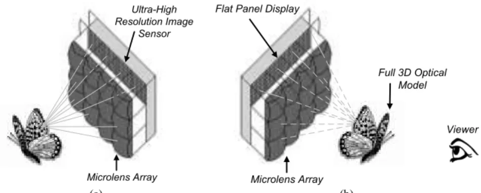
In this context, holoscopic imaging – also known as integral, light field, and plenoptic imaging – derives from the fundamentals of light field sampling, where not only spatial information about the 3D scene can be captured but also angular, i.e., the “whole observable” (holoscopic) scene. As a result of the used optical system, known as a “fly’s eye” microlens array [4] (as shown in Fig. 1), the 3D holoscopic technology allows: i) capturing a dense number of views with smooth motion parallax in both horizontal and vertical directions [4], ii) reducing the eye fatigue due to more natural convergence-accommodation cues[5].

Recently, holoscopic imaging has become a promising approach for 3D imaging and sensing, being applied in many different areas of research, such as 3D television [6], image recognition and medical imaging [5]. Moreover, novel initiatives on

* Corresponding author. Tel.: +351 218418164.

E-mail address: caroline.conti@lx.it.pt.

(a) (b)

Fig. 1 A holoscopic imaging system: (a) acquisition side; (b) display side Microlens Array

Ultra-High Resolution Image

Sensor

Microlens Array Flat Panel Display

Viewer Full 3D Optical

image and video coding standardization have also considered 3D holoscopic application scenarios, notably: the JPEG working group started recently a new study activity – known as JPEG Pleno [7] – targeting richer image capturing, visualization, and manipulation; the MPEG group started the third phase of Free-viewpoint Television (FTV), in August 2013, targeting super multiview, free navigation and full parallax imaging applications [8].

Naturally, the future success of 3D holoscopic video applications in the consumer’s market depends on how well various challenges in this type of systems will be overcome. Providing an efficient coding scheme to deal with the large amount of data involved in such systems is a requirement of utmost importance, and will be the main focus of this paper. Although the state-of-the-art HEVC [9] standard is able to fulfill current requirements for high and ultra-high resolution 2D video content, it does not comprise adequate coding tools for the inherent characteristics of 3D holoscopic video content. In fact, in [10], the authors have already presented preliminary results that show that further performance improvements relatively to HEVC can be reached for 3D holoscopic image coding. This is possible by making use of a self-similarity (SS) compensated prediction.

While addressing the aforementioned challenges, this paper proposes an efficient 3D holoscopic codec for Intra and Inter coding based on HEVC. This solution makes use of the SS compensated prediction to efficiently explore the inherent correlation of the 3D holoscopic content in Intra- and Inter-coded frames. Furthermore, a novel vector prediction scheme is also proposed to take advantage of the distinctive characteristics of the SS prediction data. The proposed prediction scheme is not tuned for any particular optical system since it does not require any explicit knowledge about it (e.g., microlens’ size, focal length, and distance of the microlenses to the image sensor).

In addition, relevant 3D holoscopic coding schemes proposed in the literature are reviewed and compared against the proposed solution. To do this, an extensive analysis of the proposed codec for Intra and Inter coding is also provided.

The remainder of this paper is organized as follows. Section 2 reviews the major concepts of holoscopic imaging. Section 3 presents a literature review in terms of 3D holoscopic image and video coding solutions. Section 4 presents the proposed codec architecture for 3D holoscopic video coding based on HEVC, including an efficient SS vector prediction to further improve the proposed coding solution. Section 5 presents test conditions and experimental results; and, finally, Section 6 concludes the paper.

2. Holoscopic Imaging Technology

In order to better understand the relevant aspects for 3D holoscopic image and video coding, this section overviews the principles behind the holoscopic imaging approach, as well the intrinsic correlations existing in this type of content.

2.1. Principles of holoscopic imaging

The concepts behind holoscopic imaging were firstly proposed by G. M. Lippmann and referred to as integral photography in 1908 [11]. Briefly, the holoscopic imaging system comprises a regularly spaced array of small microlenses, known as a “fly’s eye” lens array [1], which is used for both acquisition and display of the 3D holoscopic images, as can be seen in Fig. 1. At the acquisition side (Fig. 1a), the light beams coming from a given object with various incident angles are firstly refracted through the microlens array to be, then, captured by the 2D image sensor. Hence, each microlens works as an individual small low resolution camera conveying a particular perspective of the 3D object at slightly different angles. At the display side (Fig. 1b), a similar optical setup can be used, where a simple flat panel display is used to project the recorded 3D holoscopic image through the microlens array. Then, the intersection of the light beams passing through the microlenses recreates a full 3D optical model of the captured object, which can be observable without the need for special glasses.

As a result of the used optical system, the planar light intensity distribution representing a 3D holoscopic image corresponds to a 2D array of micro-images, as illustrated in Fig. 2, where both light intensity and direction information are recorded. Furthermore, several packing schemes, shapes and sizes of microlenses are possible in the array, as can be seen in Fig. 3, and the structure of the micro-images is a consequence of the chosen microlens array.

Regarding the inherent redundancy in 3D holoscopic content, although there is a resemblance with 2D content, an analysis of its autocorrelation function (in Fig. 4) reveals inherent correlations that are not exploited by state-of-the-art 2D video coding solutions. Notably, in the spatial domain, the pixel correlation in 3D holoscopic content is not as smooth as in conventional 2D video content, presenting a periodic structure of approximately one micro-image size (represented in each direction by  and

 in Fig. 4b). Additionally, each micro-image itself has some degree of inter-pixel redundancy as is also common in 2D images.

On the other hand, as in conventional 2D video, a 3D holoscopic video consists of a temporal sequence of frames with motion (e.g., object or camera motion). Consequently, the holoscopic video sequence can be represented more efficiently by exploring not only the spatial correlation inside each frame, but also the temporal correlation between successive frames.

However, since each micro-image contains a different perspective of the same scene from slightly different angles, this high temporal correlation occurs between micro-images in the same position in successive frames and also across micro-images in different positions (in successive frames).

2.2. Other data arrangements for holoscopic content

As will be seen in Section 3, some coding schemes in the literature propose to re-arrange the 3D holoscopic data to explore its intrinsic correlations. In this context, there are two relevant data arrangements that will be briefly reviewed in this section, based on viewpoint images and ray-space images.

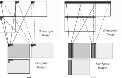
A viewpoint image represents an orthographic projection of the complete (captured) 3D scene in a particular direction. As can be seen in Fig. 5a, a viewpoint image is simply constructed by extracting one pixel with the same relative position from each micro-image of a given 3D holoscopic frame.

It is also possible to re-arrange the 3D holoscopic data as an array of all viewpoint images, as illustrated in Fig. 6a. The resulting image is here referred to as VI-based holoscopic image.

Additionally, the epipolar-plane technique [12] can be used to generate ray-space images from the 3D holoscopic content. A ray-space image can be formed by stacking together micro-images in the same row/column (in the array of microlenses) and,

(a) (b)

Fig. 2 3D holoscopic image captured with a 250 µm pitch microlens array: (a) full image with resolution of 1920×1088; (b) enlargement of 280×224 pixels showing the array of micro-images

(a) (b) (c)

Fig. 3 Possible microlens array’s structures: (a) honeycomb-packed, hexagonal shaped lenses; (b) rectangular-packed, circular-shaped lenses with different focal lengths; and (c) rectangular-packed, squared-shaped lenses

(a) (b)

Fig. 4 Example of inherent 3D holoscopic spatial correlation: (a) autocorrelation function for a 3D holoscopic image; and (b) projection onto x and y axis, showing the high correlation between points spaced of about one micro-image size (× )

-MIj 0+MIj 1.12 1.22 1.32 1.42 x 104 x 2 D co rr (H I) -MIi 0+MIi 1.119 1.219 1.319 1.419 x 104 y 2 D c o rr (H I)

then, taking a slice from a particular horizontal plane (perpendicular to the micro-image plane). As can be seen in Fig. 5b, this process corresponds to take one line of each micro-image in the same row in the array and to stitch them together to form a different ray-space image. In this case (Fig. 5b), the angular information across different micro-images in the horizontal direction is represented. Similarly to the VI-based holoscopic image, it is possible to re-arrange the 3D holoscopic data as an array of all ray-space images, as shown in Fig. 6b. The resulting image is here referred to as RI-based holoscopic image

It is possible to see by the enlargement (right side of Fig. 6a and Fig. 6b) that these images also present a repetitive structure, which may be alternatively exploited.

3. Review of 3D Holoscopic Image and Video Coding Schemes

Several image and video coding schemes have been proposed in the literature for 3D holoscopic content and try to take advantage of its peculiar planar intensity distribution.

For still images, the coding schemes proposed in the literature can be clustered in three main types of approaches: i) transform-based image coding, ii) pseudo video sequence coding, and iii) non-local spatial predictive image coding. For 3D

(a) (b)

Fig. 5 Process to construct viewpoint images (a), and ray-space images (b) from a 3D holoscopic image

Holoscopic Image Viewpoint Images Ray-Space Images Holoscopic Image (a) (b)

Fig. 6 Alternative data arrangements for 3D holoscopic images: (a) VI-based holoscopic image (left) and its enlargement (right); and (b) RI-based holoscopic image (left) and its enlargement (right)

holoscopic video, not many schemes have been proposed in the literature, being limited to a few multiview-based video coding schemes. Coding schemes in each of the distinguished groups are briefly reviewed as follows.

· Transform-based image coding: Most of the firstly proposed coding schemes for 3D holoscopic image coding are based on the discrete cosine transform (DCT) [13–15]. In these schemes, a 3D-DCT is applied to a stack of several micro-images so as to exploit the existing spatial redundancy within each image, as well as the redundancy between adjacent micro-images. The resulting transform coefficients are then quantized and entropy coded. In alternative to the DCT, other coding schemes are based on the discrete wavelet transform (DWT) [16,17]. For instance, in [17], the 3D holoscopic image is decomposed into viewpoint images, and a 3D-DWT is applied to a stack of them. Thus, the lower frequency bands are transformed using a two-dimensional discrete wavelet transform (2D-DWT) followed by arithmetic encoding, while the remaining high frequency coefficients are simply quantized and arithmetic encoded. In [18], a hybrid compression scheme is presented, which applies a 2D-DWT to each individual micro-image followed by a 2D-DCT applied to sets of DWT coefficients from neighboring micro-images. Moreover, in [19], the author proposes to encode stacks of micro-images, viewpoint images, and ray-space images (referred to as pseudo volumetric images) using JPEG2000 Part 10 [20]. After these transform-based coding schemes have been proposed in the literature, it has been since demonstrated that HEVC [9] also presents significant improvements in compression performance compared to the state-of-the-art in still image compression technology [21], showing that currently both still images and moving pictures can be efficiently compressed by using the very flexible predictive coding tools of HEVC.

· Pseudo video sequence coding: Alternatively, other compression methods propose to ‘look’ to the stack of micro-images, viewpoint images or ray-space images as a low resolution pseudo video sequence (PVS) and to encode it using a standard video encoder such as MPEG-2 [22], in [23,24], and H.264/AVC [25], in [19]. In these schemes, various scanning topologies to order the PVS are considered (raster, parallel, zigzag, spiral, and Hilbert). Generally, if the resolution of micro-, viewpoint or ray-space images is considerably smallmicro-, the coding performance using PVSs may be negatively affected by a large amount of header information and increased complexity. Notice that, when considering PVS of viewpoint images, this approach becomes very similar to the multiview-based coding schemes, although it is restricted to still image coding only. · Non-local spatial predictive image coding: This category corresponds to encode the entire 3D holoscopic image by using a

special prediction scheme to exploit the non-local spatial redundancy between different micro-images. The authors firstly proposed a scheme for self-similarity estimation and compensation in [26] to improve the performance of the H.264/AVC for 3D holoscopic image coding. In [10], the authors proposed to introduce the self-similarity compensated prediction into HEVC to take advantage of the flexible partition patterns used in this video codec. A similar prediction scheme, referred to as Intra Block Copy (IntraBC) prediction [27], has been lately proposed in the context of screen content coding (rather than 3D holoscopic video coding). This prediction scheme has been considered in the current HEVC range extension developments [28,29] with some fast algorithm implementations (e.g., by limiting partition patterns and sizes, and restricting the search window) to decrease the encoder complexity. More recently, in [30], the authors investigate alternative non-local spatial prediction, and also propose to include a prediction framework based on locally linear embedding into HEVC for 3D holoscopic image coding.

· Multiview-based video coding: Some coding schemes propose to decompose the 3D holoscopic video into several viewpoint sequences to be represented as a multiview video [31–33]. In [31], a coding scheme based on an evolutionary strategy is proposed to jointly exploit temporal motion and disparity between adjacent viewpoint images. Similarly, in [32,33], the sequence in each viewpoint is encoded using multiview video coding (MVC) [34] by defining different scanning orders. A common characteristic of these coding schemes is that they usually consider computer generated sequences with only a small numbers of VIs (up to 9). However, this number is substantially higher for natural 3D holoscopic content (usually, more than 50). Consequently, these coding schemes become much more complex and with a larger amount of header information.

4. Proposed Self-similarity Compensated Prediction Scheme for 3D Holoscopic video coding

Since a 3D holoscopic video is, actually, a sequence of 2D frames (as explained in Section 2), a simple coding approach by using a regular 2D video encoder, such as HEVC [9], can be also used. In this sense, the inherent spatial cross-correlation between neighboring micro-images in 3D holoscopic content can be seen as a type of spatial redundancy, referred to as self-similarity. This inherent correlation can then be exploited by a self-similarity (SS) compensated prediction [26] for improving coding efficiency. In the past, the idea of exploiting non-local spatial correlations has also been proposed for 2D images and

video in order to further enhance the performance of H.264/AVC intra prediction. Examples are the intra displacement compensation technique [35], and the method called template matching prediction proposed by T. K. Tan et al. [36].

This section proposes an efficient coding solution for 3D holoscopic image and video content which is based on HEVC architecture. The proposed codec using the SS compensated prediction is described, as well as an efficient vector prediction method is proposed.

4.1. Proposed Codec Architecture

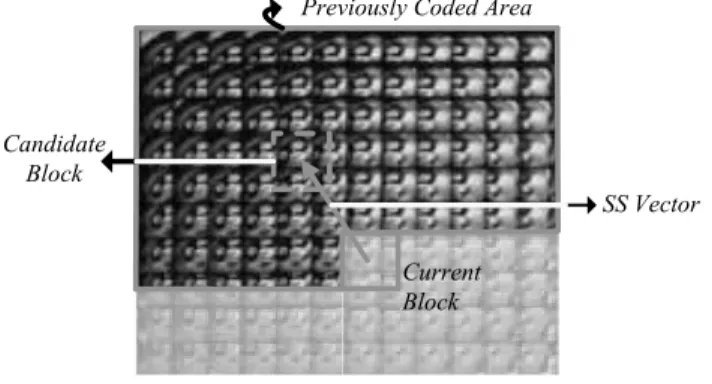
As illustrated in Fig. 7, the SS estimation process uses a block-based matching over the previously coded and reconstructed area of the current picture, to find a best match – in terms of a suitable matching criterion, such as Sum of Absolute Differences (SAD) (as used in HEVC), and Sum of Square Differences (SSD) – for prediction of the current block. As a result, the chosen block becomes the candidate predictor and the relative position between the two blocks is derived as an SS vector (similarly to a motion vector). Furthermore, the previously coded and reconstructed area of the current frame itself forms the referred SS reference frame.

The advantage of this prediction scheme is that it explores the particular correlation of the 3D holoscopic content without requiring any explicit knowledge about the used optical system (e.g., microlens’ size, focal length, and distance of the microlenses to the image sensor). Notice that, although these parameters may be provided by camera makers, many of them are highly dependent on the manufacturing process, being different from camera to camera. For instance, the fabrication process results in microlenses that may vary slightly in shape, size, and relative position, needing a very careful and complex calibration process in the holoscopic camera. For this reason, using compression and rendering tools that are less dependent to these calibration processes would be advantageous for supporting a vaster selection of devices without increasing the complexity.

Moreover, considering a scalable video coding scenario where the base layer is HEVC-compatible, such as in [37], it is convenient from an implementation point of view that most of the syntax in the enhancement layers – supporting the holoscopic coding – be as close as possible to that of this standard codec. In addition, it is also possible to improve the prediction or to reduce the complexity of the encoding process by reusing coding information from the lower layers, similar to what has been done for the 3D and scalable extensions of HEVC.

In this sense, Fig. 8 presents the proposed 3D holoscopic codec architecture, which is based on HEVC and comprises additional and modified modules to efficiently handle the 3D holoscopic content. HEVC has demonstrated significant improvements compared to the state of the art image and video codecs, such as JPEG 2000 and H.264/AVC. This high compression performance is mainly due to the very flexible prediction modes and partition patterns. Basically, the basic unit for compression is a square 2N×2N block with up to 64×64 luma samples in size, called coding block (CB), which can be recursively split into four smaller CBs until a pre-defined minimum size is reached (which may be as small as 8×8). Each CB is encoded based on a spatial prediction (Intra Picture Prediction in Fig. 8) or temporal prediction (Motion Estimation and Compensation in Fig. 8) and the residual information (difference between the chosen predictor block and the current coding block) is them transformed and quantized. To employ these prediction modes, each CB can be further split into smaller prediction units (PU), which correspond to the basic unit that carries information related to the used prediction mode, such as the type of prediction, number of PUs, their sizes, and partition patterns.

Therefore, the proposed codec introduces an additional type of prediction mode, and the encoder will choose the best one based on the conventional RD optimization (RDO) process of HEVC. Specifically, introducing the SS compensated prediction into HEVC for Intra- and Inter-code frames includes adaptation at the following stages of the coding process:

A1.7 A3.6 A1.21

A2.1

Fig. 7 The self-similarity estimation process

SS Vector Previously Coded Area

Current Block Candidate

(1) Reference picture list construction: The conventional HEVC has two reference picture lists that are used to hold the temporal reference frames. To distinguish which temporal reference frame is in each position of the list, the Picture Order Count (POC) value or POC distance to the current picture is used.

a. To allow the SS compensated prediction in Intra-coded frames, the reference list construction and signaling need to be allowed so as to include the SS reference. This process is managed by the reference memory block in Fig. 8. The computational complexity and necessary memory for this new Intra frame are comparable to those of HEVC Inter P frames with only one active reference in the reference picture list.

b. For Inter-coded frames, since there is only one SS reference picture for each picture, no additional signaling is necessary to distinguish between a SS reference and a temporal reference picture, and the distinction is also based on the POC distance to the current picture. In the proposed coding scheme, the POC distance for the SS reference is always zero. Furthermore, extensive tests were carried out to determine the most efficient position in which to include the SS reference in the list of reference pictures. It was concluded that the list should be firstly initialized with the available short term temporal reference pictures. Hence, the SS reference is appended to the list afterwards, becoming available for prediction of the current picture. Notice that, if the number of active reference pictures is kept the same (i.e., if it is not increased by one to include the SS reference), the computational complexity load will be identical to conventional HEVC Inter-coded frames. Extensive tests were also conducted during the implementation of the proposed solution (by increasing the number of active references) and this resulted in no significant improvement in the compression efficiency. Detailed information about HEVC computational complexity can be found in [38].

(2) Prediction modes and partition patterns: For Intra-coded frames, the proposed coding scheme includes two new prediction modes, referred to as SS and SS-skip prediction modes. The SS prediction mode allows to use the eight HEVC PU partition patterns (i.e., 2N×2N, N×2N, 2N×N, N×N, 2N×nU, 2N×nD, nL×2N and nR×2N [9]). Basically, each pattern defines a flexible way to partition the coding block for evaluating the SS estimation process. These prediction modes can be evaluated for all CB sizes (i.e., from 64×64 down to 8×8) in the conventional RD optimization (RDO) process to choose the best prediction mode. In the SS-skip prediction mode, the SS vector is directly derived from the HEVC merge technique [9], used in the HEVC Inter prediction. However, the SS-skip mode restricts the SS vector candidates from only spatially neighboring PUs guaranteeing that the referenced area is limited to the area defined in the SS estimation process. This means that the prediction block signaled by the chosen SS vector is already available in the SS reference buffer at decoding time. Improvements to the conventional merge method for the SS prediction are also proposed in Section 4.2.

A1.8

A1.8 A2.1

Fig. 8 Proposed 3D holoscopic video codec architecture based on HEVC

Transform, Scaling & Quantization Scaling & Inverse Transform Reference Memory Input Video Signal -Header Formatting & CABAC Motion Data Control Data Motion Estimation Intra-Picture Prediction Motion Compensation

General Coder Control

Coded Bitstream Deblocking & SAO Filters Coefficient Data SS Estimation SS Compensation SS Data Filter Control Data Intra Data

(3) Block-based matching search: Similarly to the motion estimation, the search area is restricted in the SS estimation (Fig. 8) to minimize the computational complexity. However, due to the different nature of the SS vectors (as will be seen in Section 4.2), a larger search area than in temporal prediction of conventional 2D content may be needed so as to the SS vectors compensate the micro-image structure.

(4) SS Vector Prediction: To further improve the performance of inter prediction of HEVC, motion vectors are encoded or directly derived by calculating a predicted motion vector, based on vector candidates from PUs in a spatial or temporal neighborhood. Regarding the SS vector prediction:

a. In Intra-coded frames, an optimal prediction for each SS vector is computed for each PU partition, in RDO sense, using a scheme derived from the HEVC Advanced Motion Vector Prediction (AVMP) [9], but considering only the vector candidates from spatially neighboring CBs (since there are no candidates in co-located PU positions of the SS reference). b. In Inter-coded frames, the following restrictions are considered when constructing the vector candidates list in the

AMVP: i) the co-located candidate is not allowed for an SS reference (once more, this distinction is done by a POC difference of zero); and ii) when constructing the AMVP candidate list, only vector candidates of the same type as the current vector being coded are allowed. For instance, if the current vector corresponds to an SS reference (with a POC difference of zero), the vector candidate must correspond to an SS reference (and the same for temporal reference). Based on the inherent 3D holoscopic structure of micro-images, a novel vector prediction scheme is also proposed in Section 4.2.

4.2. Proposed MI-based prediction for self-similarity vectors

Regarding the conventional HEVC, vector prediction is used in two methods: AMVP and merge [9]. In these methods, a vector candidate (or merge candidate) list is constructed by selecting vectors from CBs in the spatial and temporal (co-located) neighborhood. If there is no available vector at neighboring CBs (e.g., if the CB was coded with an Intra prediction mode), zero vector candidates are added to fill the candidate list. From these spatio-temporal (or zero) candidates, the encoder selects the best predictor vector in a RDO sense, and transmits only the index of the chosen candidate in the list.

The definition of SS co-located CB positions is not applicable since the SS reference is the current frame itself. For this reason, in Intra-coded frames, AMVP and merge candidate lists are limited to spatial candidates only. Furthermore, zero vector candidates are never available for a SS reference – as it corresponds to a position outside the causal area of previous coded and reconstructed blocks – making the number of candidate vectors even more limited. Similarly, for Inter-coded frames, although the co-located CB in a temporal reference is still available, the derived temporal vector will only be possible to use if it is inside the causal area of the SS reference.

A1.9 A2.1

(a)

(b)

Fig. 9 SS vectors in a coded 3D holoscopic image with micro-image resolution of 28×28: (a) Distribution along the image (right); (b) Heat map showing the corresponding vector values’ distribution

0 200 400 600 800 1000 1200 1400 1600 1800 0 200 400 600 800 1000 x y -120 -100 -80 -60 -40 -20 0 20 40 60 80 100 120 -120 -100 -80 -60 -40 -20 0

However, for 3D holoscopic content, besides the possible correlation between vectors from neighboring CBs, the SS vectors present a regular distribution, which is related to the structure of the micro-images. As an example, Fig. 9a shows the distribution of the transmitted SS vectors (right) for a 3D holoscopic image with micro-image resolution of 28×28, and Fig. 9b shows a heat map of the corresponding SS vector values distribution. From this, it can be observed that the magnitude of the SS vectors is usually multiple of the micro-image resolution so as to compensate the micro-image boundaries.

Due to the specific nature of SS vectors, a set of new candidate SS vectors, referred to as MI-based SS candidate vectors, is proposed to be included into AMVP and merge methods of HEVC to further improve the proposed coding solution.

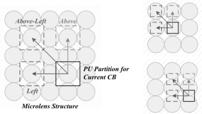
This new set includes the left MI-based vector, above MI-based vector, and above-left MI-based vector, as given by (1), (2), and (3), respectively. Where _× _ corresponds to the size of the current PU partition, and !"_#× !"_$ represents the micro-image resolution (in pixels).

The terms %_⁄!"_#' and ⌈_⁄!"_$⌉ force the candidate vectors to be distributed according to the structure of micro-images, as well as to be inside the area of previous coded and reconstructed CBs. Fig. 10 shows that the position of the three vector candidates is always related to the micro-image structure independently of the PU partition size (that can be larger or smaller than the micro-image resolution).

*+,-./012 = 3− 5  !"#6 × !"#, 0 9 (1) :+,-./012= ;0 , − <  !"$> × !"$ ? (2) :*+,-./012= 3− 5  !"#6 × !"#, − <  !"$> × !"$ 9 (3)

Finally, to introduce the proposed MI-based vector candidates into AMVP and merge methods, the following changes are needed:

(1) Allowing based candidate in AMVP: for the SS reference, after the selection of conventional vector candidates, one MI-based vector candidate is selected between the left MI-MI-based vector and above MI-MI-based vector. In the final list there are two candidates (as in [9]). As a consequence, the chosen prediction vector from this new set of candidates becomes a better starting point for the block-based matching search.

(2) Allowing MI-based candidates in merge: for the SS reference, after selecting the available conventional merge candidates, up to three MI-based merge candidates are included into the merge candidate list until the maximum number of candidates is reached. The order of selection is defined as left, above and above-left. As in [9], the maximum number of merge candidate is five. As will be shown in 5.2, adopting the proposed MI-based vector prediction into the merge method (for the SS-skip prediction mode) allows further improvements on the performance of the proposed coding solution.

Notice that, the used resolution of the micro-images !"_#× !"_$ can be an approximate value that may be easily derived from the texture information. For instance, by detecting the distance between the peaks in the autocorrelation function shown in Fig. 4, or by using a segmentation algorithm to recognize the vignetting existing at the border of the micro-images (see Fig. 2b). Moreover, this information can be derived at the encoder side and transmitted at once in the high level syntax elements of the bitstream, resulting in nearly no performance loss.

A1.21

Fig. 10 Proposed MI-based vector candidates: when the prediction block is larger (left) and smaller (right) than the micro-image resolution

Left

Above-Left Above

Microlens Structure

PU Partition for Current CB

5. Performance assessment

This section assesses the RD performance of the proposed 3D holoscopic video coding solution. For this purpose, the test conditions are firstly introduced and, then, the obtained results are presented and discussed.

5.1. Test Conditions

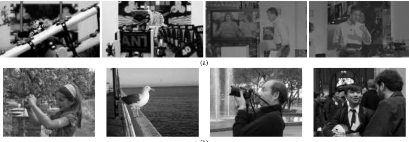
To evaluate the performance of the proposed 3D holoscopic coding solution, four different 3D holoscopic test sequences are considered: Plane and Toy, Robot 3D, Demichelis Cut, and Demichelis Spark, as well as four images, Laura, Seagull, Jeff, and Zhengyun [39] (see Fig. 11). All the sequences and images were captured using a holoscopic camera with a focused setup [40]. A detailed description about the characteristics of this test set is shown in Table 1.

For these tests, the reference software of HEVC (MV-HEVC) version 14.0 was used as the benchmark, as well as the base software for implementing the proposed codec. Therefore, the abovementioned test sequences were encoded according to the common test conditions defined in [41] as “Intra, main” and “Low-delay, main, P slices only” configurations, respectively, for Intra and Inter coding. Notice that, although other coding configurations with B slices may lead to higher compression efficiency, they are especially useful for sequences with high temporal variations [42]. For this reason, it is not expected that the introduction of B frames will change much the results for the used test sequences, since all of them have relatively low temporal information indices (see Table 1). Therefore, for Inter coding, it was considered an “IPPP...” structure with:

· Group of Pictures (GOP) size: The GOP size was fixed as 1, corresponding to an “IPPP...” GOP prediction structure. · Intra Period: The intra refresh period was 9 with the decoding refresh type Clean Random Access (CRA) [9].

· Quantization Parameter (QP) value: For Intra-coded frames the used QP values are 22, 27, 32, 37 and 42 to analyze the RD performance of the proposed codec. When analyzing the results in terms of the Bjøntegaard Delta in PSNR (BD-PSNR) and rate (BD-BR) [43], the QP values 22 and 42 were interchanged to better analyze the performance, respectively, for high and low bitrates. For the “Low-delay, main, P slices only” configuration the proposed 3D holoscopic video codec, it was observed that for the same QP there is always a slight decrease in PSNR in comparison to HEVC Intra-coded frames. This affects significantly the consecutive Inter-coded frames, which also present lower PSNR when compared to HEVC. Moreover, this might indicate that the RD model used by HEVC is not properly optimized for coding 3D holoscopic content with this new Intra-coded frame using SS modes. Therefore, since there is a significant margin in RD gains of the proposed codec compared to the HEVC Intra coding, the QP for Intra-coded frames was adjusted, as explained in [44], so that both HEVC and the proposed codec spend the same number of bits. For Inter-coded frames, the QP values are computed as defined by the reference software [41].

· Search Range: A search range value of 128 was adopted in both Intra- and Inter-coded frames for all reference types (for temporal and SS references), and the full search algorithm is also used in the both cases.

A1.12 A2.2 A3.1 A1.22 A1.13 (a) (b)

Fig. 11 Example of the central rendered view from each holoscopic test content. (a) Sequences (from left): Plane and Toy, Robot 3D, Demichelis Cut,

Additionally, in order to better assess the performance of the proposed coding scheme, a comparison between alternative objective quality metrics for decompressed 3D holoscopic content is performed as well as an analysis of the impact over the perceived quality of views synthesized from the 3D holoscopic content is also provided.

Notice that, due to the relative early stage of 3D holoscopic display technology, proposing quality evaluation metrics for this type of content is a completely open issue, and there have been only a few works addressing it in the literature. In [45], an angle-dependent metric is proposed to be compatible with the viewing characteristics of 3D holoscopic content. Instead of using the general PSNR calculated in the entire 3D holoscopic image, the average PSNR across all viewpoint images is taken, as well the corresponding minimum and a maximum margin values. In [19], two metrics are proposed for quality assessment in 3D holoscopic content visualization: sparse angle-dependent and sparse depth-dependent. In the both metrics the explicit knowledge of the optical capturing system (e.g., focal length, pitch and position of the microlens array) is used to extract views from the 3D holoscopic content at the exact position of a viewer in front of a 3D holoscopic display. In the sparse angle-dependent, the average Structural Similarity Index (SSIM) is taken in a set of five views from equidistant viewing angles (with

A3.1 A3.2

Table 1 3D Holoscopic Test Sequences and Images with a detailed description of the captured scene, camera setup and rendering parameters.

Sequence/Image Description Information for Rendering [40]

Plane and Toy*

1920×1088 at 25Hz (250 frames) Focus: patch size of 9×9 pixels to have the toy in focus

Studio scene; the plane moves closer and nearer to the

camera. (Temporal Information Index (TI) [22]: 23.33) Perspective: 9 different perspectives, corresponding to the pixel positions: { (-4,-4), (-4,0), (-4,4), (0,-4), (0,0), (0,4), (4,-4), (4,0), (4,4)}

MLA: Rectangular-arranged (Ra), squared-based lenses

Microlens: 0,25 mm (pitch), 1,0 mm (focal length) MI resolution: 28×28

Robot 3D*

1920×1088 at 25Hz (150 frames) Focus: patch size of 4×4 pixels to have the Robot in focus

Studio scene with color and ISO charts; the robot moves

and all around the scene. (TI: 26.03) Perspective: 9 different perspectives, corresponding to the pixel positions: { (-4,-4), (-4,0), (-4,4), (0,-4), (0,0), (0,4), (4,-4), (4,0), (4,4)}

MLA: Ra-MLA, squared-based lenses

Microlens: 0,25 mm (pitch), 1,0 mm (focal length) MI resolution: 28×28

Demichelis Cut*

2880×1620 at 25Hz (150 frames) Focus: patch size of 14×14 pixels to have the presenter in focus

Studio scene; the background (TV scene) continuously

changes. (TI: 33.96) Perspective: 9 different perspectives, corresponding to the pixel positions: { (-6,-6), (-6,0), (-6,6), (0,-6), (0,0), (0,6), (6,-6), (6,0), (6,6)}

MLA: Ra-MLA, semi-spherical lenses

Microlens: 0,3 mm (pitch), 2,2 mm (focal length) MI resolution: 38×38

Demichelis Spark*

2880×1620 at 25Hz (150 frames) Focus: patch size of 12×12 pixels to have the presenter in focus

Studio scene with linear camera movement. (TI:

12.4086) Perspective: 9 different perspectives, corresponding to the pixel positions: { (-6,-6), (-6,0), (-6,6), (0,-6), (0,0), (0,6), (6,-6), (6,0), (6,6)}

MLA: Ra-MLA, semi-spherical lenses

Microlens: 0,3 mm (pitch), 2,2 mm (focal length) MI resolution: 38×38

Laura

7240×5432 (1 frame) Focus: patch size of 10×10 pixels to have the girl in focus

Nature scene with a girl standing in the center Perspective: 9 different perspectives, corresponding to the pixel positions: {

(-16,-16), (-16,0), (-16, 16), (0,-16), (0,0), (0, 16), (16,-16), (16,0), (16,16)}

MLA: Ra-MLA, squared-based lenses

Microlens: 0,5 mm (pitch), 1,5 mm (focal length) [40] MI resolution: 75×75

Seagull

7240×5432 (1 frame) Focus: patch size of 9×9 pixels to have the seagull in focus

Landscape scene with a seagull in the foreground Perspective: 9 different perspectives, corresponding to the pixel positions: {

(-16,-16), (-16,0), (-16, 16), (0,-16), (0,0), (0, 16), (16,-16), (16,0), (16,16)}

MLA: Ra-MLA, squared-based lenses

Microlens: 0,5 mm (pitch), 1,5 mm (focal length) [40] MI resolution: 75×75

Jeff

7240×5432 (1 frame) Focus: patch size of 11×11 pixels to have the photographer in focus

Outside scene with transparent and reflecting objects Perspective: 9 different perspectives, corresponding to the pixel positions: {

(-16,-16), (-16,0), (-16, 16), (0,-16), (0,0), (0, 16), (16,-16), (16,0), (16,16)}

MLA: Ra-MLA, squared-based lenses

Microlens: 0,5 mm (pitch), 1,5 mm (focal length) [40] MI resolution: 75×75

Zhengyun

7240×5432 (1 frame) Focus: patch size of 9×9 pixels to have the man in the center in focus

Inside scene (two different light sources) with people in

different depth positions Perspective: 9 different perspectives, corresponding to the pixel positions: { (-16,-16), (-16,0), (-16, 16), (0,-16), (0,0), (0, 16), (16,-16), (16,0), (16,16)}

MLA: Ra-MLA, squared-based lenses

Microlens: 0,5 mm (pitch), 1,5 mm (focal length) [40] MI resolution: 75×75

fixed distance to the microlens array). In the sparse depth-dependent, depth information is estimated and an average PSNR is taken in a rendered view (with fixed angular position) over sets of pixels in different depth layers. In [24], a micro-image deviation-dependent metric is proposed. Based on the fact that the viewed 3D object is formed by the intersection of the light beams passing through neighboring microlenses, the average PSNR and standard deviation across all micro-images are calculated.

Therefore, to accomplish this additional comparison, the following methodology was defined:

(1) Use case definition: This analysis will consider prospective 3D application services that may use a 3D holoscopic display in the future for a more immersive visualization (e.g., medical imaging, industrial manufacturing, and gaming), or FTV applications where views are synthesized from the 3D holoscopic content. Notice that, to reduce the degrees of freedom in this analysis, only algorithms that do not need interpolation for generating the views (or viewpoint images) are considered. However, since rendering views from the 3D holoscopic content may induce new types of artifacts, the reliability of these quality assessments need to be studied more carefully in the future by comparing them with subjective quality scores. (2) Quality metrics selection: Three alternative metrics are used and compared to the PSNR over the entire 3D holoscopic

image:

a. Angle-dependent PSNR: In this case the metric proposed in [45] is used, as given in (4) for all  ×  viewpoint images of a 3D holoscopic image. Since it is possible to establish a relationship between the viewpoint image and the reconstructed scene that a user (who is at a particular viewing position) would see with a holoscopic display [46], this metric tries to directly analyze the quality of this visualized 3D object. However, notice that as any rendering algorithm, constructing viewpoint images may produce other undesirable artifacts that will also affect the subjective quality of the visualized 3D object. In this case, the texture resampling from micro-images to the viewpoint images usually results in very low resolution images with severe aliasing artifacts [46].

b. MI-deviation PSNR: In this case the metric proposed in [24] is used, as given in (5) for all  ׁ micro-images of a 3D holoscopic image. As discussed in [24], the idea behind this metric is that the quality of the visualized 3D object by using a holoscopic display will be affected by drastic variations on the quality of neighboring micro-images. However, it should be also noted that the MIs contains only a small portion of the captured scene that will be never visualized directly, being difficult to correlate with a subjective quality assessment.

!" ########_Angl-dep.= 1 ! × $ % % !"&,' ( ')* + &)* /Angle-dep.= 0% % !"&,'2 ( ')* − !"########_Angle-dep.2 + &)* (4) !" ########_MI-dev. =_{ ×  % % !"}1 4,5 6 5)* 7 4)* /MI-dev.= 0 % % !"4,52 6 5)* − !"########_MI-dev.2 7 4)* (5)

c. Rendering-dependent SSIM: Similarly to the metric proposed in [19], the average (and also the standard deviation) SSIM is calculated from a set of 8 views rendered from the 3D holoscopic image, as given in (6). However, the algorithm proposed in [40], referred to as Basic Rendering, is used to generate the views instead of the one used in [19] (since usually there is no information about the used optical system and to avoid interpolation). This algorithm allows selecting a particular perspective and plane of focus (i.e., which image plane will appear in sharp focus) in the generated 2D view. Therefore, this metric is used to provide a better correspondence with the quality perception expected by a user positioned in front of a 3D holoscopic display as well as the quality of synthesized views for FTV applications. Note that any rendering algorithm may be used, and each of them will introduce different degradation that also affect the subjective quality of the synthesized view.

A1.15

A1.15

!!9 #######_:;5<-dep.= 1 8 % !!9> ? >)* /:;5<-dep.= 0 % % !!9>2 6 5)* − !!9#######_:;5<-dep.2 7 4)* (6)

(3) Solution assessment: Due to resource issues (there is no commercially available 3D holoscopic display to employ subjective tests), extensive subjective quality assessment is not employed to validate the tested objective metrics. Moreover, since there is still no consensus regarding evaluation methodologies for 3D holoscopic content, results for synthesized views are shown as a qualitative analysis of the proposed coding solution. An alternative would be to perform the subjective evaluation by view sweeping or using a stereo or multiview display. However, this is left for future work.

5.2. Experimental Results for Intra Coding

Although the SS compensated prediction is able to explore the intrinsic correlation between neighboring MIs to improve the coding performance, it is also important to understand how the intrinsic correlations of this type of content depend on the way the 3D holoscopic data is arranged. As described in Section 2.2, besides the representation based on a micro-images array, it is also possible to arrange the 3D holoscopic data as viewpoint images or ray-space images.

Therefore, in order to investigate how advantageous these different arrangements are in terms of the RD performance of the prediction scheme, four solutions are tested and compared:

(1) HEVC: The original 3D holoscopic image is encoded using HEVC with “Intra, main” configuration [41].

(2) 3DHolo: The original 3D holoscopic image is encoded using the proposed Intra coding scheme with SS compensated prediction.

(3) VI-based 3DHolo: The original 3D holoscopic image is re-arranged so as to generate the corresponding VI-based holoscopic image, which is then coded with the proposed 3DHolo coding scheme. Since, in most of the cases, generated VIs have higher resolution than the corresponding MIs, areas with significant correlation will be further apart. Therefore, larger search ranges are allowed for the SS estimation. In this case, the search range used for the 3DHolo solution (128) is multiplied to ratio between the viewpoint image resolution to the micro-image resolution.

(4) RI-based 3DHolo: The original 3D holoscopic image is re-arranged so as to generate the corresponding RI-based holoscopic image, which is then coded with the proposed 3DHolo coding scheme. In this case, the search range is also multiplied to the ratio between the ray-space image resolution to the micro-image resolution.

The RD performance is also compared to solutions where the 3D holoscopic image is decomposed into PVS (or multiview) content [19,23,24]. For a fair comparison, the following three coding solutions are tested:

(1) MI-based PVS: A PVS of micro-images is coded using HEVC. Since the resolution of each micro-image is considerably smaller than HEVC commonly supported resolutions, the largest CB size was set to 16×16. The MI-based PVS is then encoded using an “IPPP...” configuration. Various MI scanning orders were tested (raster, parallel, zigzag, and spiral), but only the spiral order is presented as it achieved the best performance.

(2) VI-based PVS: A PVS of viewpoint images is encoded with HEVC. After testing various orders for scanning the viewpoint images, the spiral order is presented as it achieved the best performance. In HEVC, the largest CU is set to 16×16 and an “IPPP...” configuration is also used.

(3) RI-based PVS: A PVS of ray-space images is encoded with HEVC using the same configuration of the previous two solutions.

In order to assess the RD performance for different non-local spatial prediction schemes, the 3DHolo solution is also compared to the following two coding solutions for screen content coding:

(1) HEVC RExt 6.0: The original 3D holoscopic image is encoded using the Range Extension HEVC reference software version 6.0 [28], where IntraBC prediction is used. Based on the characteristics of the screen content, the complexity of IntraBC prediction was reduced in this solution, mainly due to: i) the smaller number of allowed PU partition patterns (only 2N×2N, N×2N, 2N×N, N×N); ii) limited CB sizes (CBs larger than 16×16 are skipped, based on a threshold on RD cost); iii) the use

of only one dimensional (1D) vectors for 16×16 CBs; iv) the use of integer block matching search across only one or more CBs to the left; v) the usage of a default vector predictor instead of AMVP (the vector of the latest coded CB).

(2)HEVC SCC 1.0: The original 3D holoscopic image is encoded using the screen content coding extension of HEVC, reference software SCC 1.0 [29]. Some improvements in performance for screen content coding were proposed in this solution compared to the HEVC RExt 6.0. Notably, the search window was expanded over the entire CB row or column (for 16×16 CBs), and over some positions in the entire picture by using a hash-based search (for 8×8 CBs).

The RD performance is assessed in terms of luma Peak Signal to Noise Ratio (PSNR) versus average bits per pixel (bpp) by using the first frame from each 3D holoscopic test sequences (see Table 1). Fig. 12 shows the RD performance for each tested image.

Additionally, to illustrate the effectiveness of the 3DHolo solution (with MI-based vector prediction), a comparison against HEVC, HEVC RExt 6.0, HEVC SCC 1.0, and 3DHolo without MI-based vector prediction, referred to as 3DHolo w/o MIvp, coding solutions is presented in Table 2. The results are shown in terms of the Bjøntegaard Delta in PSNR (BD-PSNR) and rate (BD-BR) for low bitrates [43]

From the results in Fig. 12 and Table 2, the following conclusions can be drawn.

· Results for different data arrangements: From the results presented in Fig. 12, it is possible to conclude data arrangements based on micro-images (i.e., MI-based PVS, HEVC RExt 6.0, HEVC SCC 1.0, and 3DHolo solutions) are considerably more efficient than the corresponding viewpoint and ray-space image arrangements. A careful analysis has shown that the resampling process from the captured micro-images to viewpoint and ray-space images resulted in images with significant aliasing artifacts, which are then difficult to predict and to compress. Analyzing and comparing the DCT coefficients of these images, it was seen that the viewpoint images presented significant high frequency energy. The same happens with the ray-space images mainly along the horizontal axis (that corresponds to the direction used to arrange the angular information, as seen in Fig. 5b). Therefore, as observed in Fig. 12, viewpoint and ray-space image arrangements lead to a significant drop in PSNR values at lower bpp since the high frequency DCT coefficients are more coarsely quantized. On the other hand, at higher bpp, the needed number of bits considerably increases for encoding these high frequency coefficients.

· Results for different coding schemes: Comparing the performance for solutions based on the micro-image arrangement (i.e., HEVC, 3DHolo, HEVC RExt 6.0, HEVC SCC 1.0), in Fig. 12 and Table 2, it is possible to conclude that coding solutions that somehow exploit the inherent correlation of the 3D holoscopic content (i.e., 3DHolo, HEVC RExt 6.0, HEVC SCC 1.0) lead to a better RD performance compared to the conventional HEVC (with gains up to 3.54 dB / -55.26 %).

A1.12 A3.8 A3.4

(a) (b) (c)

(d) (e) (f)

Additionally, the proposed 3DHolo solution always outperforms HEVC RExt 6.0 and HEVC SCC 1.0, mainly when using the MI-based vector prediction (see Table 2), with significant gains and bitrate savings in average when compared to both HEVC RExt 6.0 (1.40 dB / -26.76 %) and HEVC SCC 1.0 (0.77 dB / -16.89 %). Regarding the MI-based PVS solution, although it presented significant better RD performance compared to the other PVS representations, it is still always outperformed by HEVC SCC 1.0.

· Results for different camera parameters and type of scenes: From the results in Fig. 12 and Table 2, it was observed that, the performance of the proposed 3DHolo solution seems to be more related to the used camera parameters than to the scene type. This may indicate that the more optimized for the camera parameters the coding process is, the better the compression efficiency of the solution will be.

· Results for MI-based vector prediction: on Table 2, it can be seen that by using MI-based vector predictions it is possible to improve the RD performance of the 3DHolo solution, leading to further bitrate savings (up to -8.27 %, -4.46 % in average) and coding gains (up to 0.30 dB, 0.18 dB in average) compared to 3DHolo w/o MIvp.

· Computational Complexity: Although the computational complexity of the proposed 3DHolo solution is comparable to HEVC Inter-coded frames, the encoder complexity is still a limitation when compared to fast search schemes, such as the proposed for IntraBC prediction in HEVC RExt 6.0 and HEVC SCC 1.0. Table 3 compares the encoding complexity of the 3DHolo, regarding the HEVC RExt 6.0 and HEVC SCC 1.0 solutions in terms of  _) !"#$%&'(. For these

results, a machine with a Core i7-860 processor at 2.80 GHz with 16 GB of RAM and Windows 7 64-bits operating system was used. Moreover, the results were obtained by using the same software conditions (i.e., Visual Studio C++ compiler version 9.0, and optimization parameters on). As seen in Table 3, the 3DHolo solution is the most complex encoding process (in average, 14.14 times compared to HEVC RExt 6.0, and 8.03 times compared to HEVC SCC 1.0) mainly due to the full search that was employed for the SS prediction. However, notice that the RD gains of the 3DHolo solution compared to the HEVC RExt 6.0 (1.40 dB and -26.76 % in average) and the HEVC SCC 1.0 (0.77 dB and -16.89 % in average) are not negligible, showing the importance of considering the characteristics of the 3D holoscopic content for proposing a more suitable low complexity coding solution. For instance, a fast search approach can still be studied by taking advantage of the proposed MI-based SS vectors to efficiently decrease the search window in the SS estimation. Since the development of fast coding solutions is not a normative concern, it is not a target issue in this paper and it will be left for future work.

A1.23 A3.6

A3.2

A1.23

Table 3 Encoding complexity of 3DHolo solution.

Name HEVC RExt 6.0 HEVC SCC 1.0

Plane and Toy 7.19 6.70

Robot 3D 9.13 7.62 Demichelis Cut 17.38 15.96 Demichelis Spark 13.59 13.03 Laura 10.27 0.98 Seagull 19.50 2.30 Jeff 13.25 5.11 Zhengyun 25.39 14.11 Average 14.46 8.23

Table 2 BD-PSNR and BD-BR performance for Intra coding when introducing MI-based vector candidates into AMVP and merge methods into the proposed 3D holoscopic coding solution (QPs 27, 32, 37, and 42)

Name 3DHolo vs. HEVC

3DHolo vs. HEVC RExt 6.0

3DHolo vs.

HEVC SCC 1.0 3DHolo vs. 3DHolo w/o Mivp

BD-PSNR BD-BR BD-PSNR BD-BR BD-PSNR BD-BR BD-PSNR BD-BR

Plane and Toy 1.11 dB -15.32 % 0.47 dB -6.91 % 0.41 dB -6.17 % 0.18 dB -2.76 %

Robot 3D 1.02 dB -12.71 % 0.22 dB -2.94% 0.14 dB -1.89 % 0.04 dB -0.57 % Demichelis Cut 2.38 dB -42.37 % 1.19 dB -27.16 % 0.69 dB -18.82% 0.18 dB -5.16 % Demichelis Spark 2.44 dB -47.55 % 1.34 dB -31.32 % 0.99 dB -24.81 % 0.30 dB -8.27 % Laura 2.82 dB -42.69 % 1.82 dB -31.32 % 0.75 dB -15.14 % 0.11 dB -2.48 % Seagull 3.54 dB -55.26 % 2.22 dB -40.80 % 1.10 dB -24.12 % 0.27 dB -6.63 % Jeff 2.81 dB -43.80 % 2.06 dB -36.22 % 1.09 dB -21.92 % 0.21 dB -4.67 % Zhengyun 2.63 dB -47.12 % 1.87 dB -37.39 % 0.95 dB -22.23 % 0.20 dB -5.16 % Average 2.34 dB -38.35 % 1.40 dB -26.76 % 0.77 dB -16.89 % 0.18 dB -4.46 %

5.3. Experimental Results for Different Objective Quality Metrics

In order to compare the performance of the 3DHolo solution for different quality metrics, the Intra coding results for the best four coding solutions (i.e., 3DHolo, HEVC SCC 1.0, HEVC RExt 6.0 and HEVC) are shown in Fig. 13 in terms of Angle-dependent, MI-deviation and Rendering-dependent. Additionally, Fig. 14 illustrates a portion of a central view rendered from Demichelis Spark and Laura, which were coded with the different coding solutions at same bitrate.

For the Rendering-dependent metric, a set of nine views were rendered at different positions (i.e., at central, top, left, right, bottom, top-left, top-right, bottom-left, and bottom-right) by the Basic Rendering algorithm [40]. The plane of focus was selected so as to have the main object “in focus”.

From the results in Fig. 13 and Fig. 14, the following conclusions may be derived.

· Comparison between the different objective metrics: It is possible to see, in Fig. 13, that there is a correlation between the coding performances using the three metrics, as well as a correlation with the results presented in Fig. 12 in terms of PSNR over the entire 3D holoscopic image. Considering all metrics, the proposed 3DHolo solution outperforms the other tested solutions. It was observed that MI-deviation and Angle-dependent metrics presented larger standard deviation values for all tested coding solutions. From a more careful analysis regarding the Angle-dependent metric, it was observed that viewpoint images taken from the border positions of the micro-images presented smaller PSNR values than viewpoint images from more central positions. This is related to the poor illumination at the peripheries of the micro-images (which results in a vignetting effect). As a consequence, in the peripheries of micro-images, the pixel values are spread over a wider range, which corresponds to an increase in the amount of higher frequency content. Since for a given QP, the quantization will be more aggressive for higher frequencies than for lower ones [9], the pixels in these regions will end up being more degraded (i.e., with lower PSNR values). Regarding the MI-deviation metric, since each micro-image contains only a small portion of the scene with very low resolution, the compression performance might vary considerably between micro-images that contain more homogeneous or more complex texture patterns. For instance, due to the very small resolution of each micro-image of Plane and Toy, it was observed that some of the micro-image samples (mainly in the black areas of the image) that are in homogeneous areas presented nearly nil error, thus abruptly increasing the 

MI-dev. value. This may indicate

that both these metrics should be considered locally, or in a particular spatial (for the MI-deviation metric) or angular (for the Angle-dependent metric) region of interest.

· Comparison with visual quality of rendered views: As illustrated in Fig. 14, there is also a correlation between the compared metrics and the visual quality of a view rendered from the coded reconstructed image. As it can be seen, the 3DHolo solution significantly improved the visual quality of the rendered view when compared to HEVC for the same bitrate.

· Comparison between PSNR- and SSIM-based results: Fig. 14 also presents, below each depicted image, the Rendering-dependent metric in terms of the SSIM and PSNR value of the central view rendered from the coded and reconstructed holoscopic image. These values are used as an illustrative example to compare the results in terms of PSNR- and SSIM- based metrics for coded 3D holoscopic images. From the results, it was observed that the variations in the SSIM values are considerably small compared to the actual variations in the perceived quality of the rendered view. For instance, comparing the central view of Demichelis Spark (Fig. 14, top) when encoded with 3DHolo (Fig. 14b) and HEVC (Fig. 14c), it is possible to perceive a significant degradation from the view in Fig. 14b to the view in Fig. 14c, while the variation in the SSIM value appears only in the second decimal place (0.042) in this case. In the same example, it is possible to see that although the PSNR values are high in the both cases (compared to the results for Laura in the bottom), there is an attenuation of 2.7dB from Fig. 14b to Fig. 14c

5.4. Experimental Results for Inter Coding

To assess the performance of the proposed 3D holoscopic coding solution for Inter-coded frames, the proposed 3DHolo solution is compared against HEVC codec. The RD performance is measured in terms of BD-PSNR and BD-BR [43] against HEVC and presented in Table 4 for each test sequence, and in Fig. 15 in terms of PSNR versus bitrate (bits per second).

From the results in Table 4, it can be seen that the proposed 3DHolo scheme always outperforms HEVC with gains of 0.35 dB and -7.93 % in average (for all test sequences). Moreover, as shown in Fig. 15 and Table 5, the proposed 3DHolo solution presents significantly better performance at lower bitrates, where the gains are 0.92 dB and -22.90 % in average.

In addition to these results, Table 6 shows the BD-PSNR and BD-BR performance without using the QP-adjustment for Intra-coded frames (as explained in Section 5.1).

A3.3 A3.3

A1.12 A3.2 A3.8 (a) (b) (c) (d) (e) (f)

Fig. 13 RD performance using alternative quality metrics for Intra-coded frame of: (a) Plane and Toy; (b) Demichelis Spark; (c) Laura,;(d) Seagull; (e) Jeff; and (f) Zhengyun

It can be observed that, in some cases, the overall performance of the proposed 3DHolo solution is shown to be further improved when a QP-adjustment is used. For instance, the BD results for the sequence Robot 3D are improved from -0.43 dB / -8.22 %, without QP-adjustment (Table 6), to 0.83 dB / -15.37 % (Table 5). This can be explained by the consequent improvement in quality of Intra-coded frames that are used as reference. This fact is illustrated in Fig. 16, for a portion of the central view rendered from a first Inter-coded frame of Demichelis Spark using 3DHolo w/o QP-adjustment (Fig. 16a) and using the 3DHolo (Fig. 16b). Notice that, the coding artifacts are especially more evident on the man’s face when using 3DHolo w/o QP-adjustment.

Therefore, this suggests that the RD optimization used in HEVC is not appropriate for 3D holoscopic video coding, since it is not able to find the best balance between rate and distortion constraints.

5.5. Future Research Directions

The proposed 3DHolo solution has shown that it is possible to provide efficient compression for holoscopic content even if the used camera parameters are unknown. However, with the current generation of holoscopic cameras, it will be also possible to use this type of information to further improve the holoscopic coding performance. Therefore, future work will include the study of alternative representation formats that decrease the transmitted data by making use of camera parameters, as well as

A3.6 A3.3

SSIM = 0.918, and PSNR = 37.45 dB SSIM = 0.876, and PSNR 34.75 dB

SSIM = 0.836, and PSNR = 29.78 dB SSIM = 0.716, and PSNR = 26.91 dB

(a) (b) (c)

Fig. 14 Comparison of a portion from the central 2D view of Demichelis Spark (top) and Laura (bottom) when rendering from: (a) the original image; (b) encoded and reconstructed frame using 3DHolo; (c) encoded and reconstructed frame using HEVC. The corresponding SSIM and PSNR values

(Rendering-dependent) are also shown for the two test images at around 0.0682 bpp for Demichelis Spark, and 0.1808 bpp for Laura

Table 4 BD-PSNR and BD-BR performance for Inter coding with the proposed 3D holoscopic codec

Sequence name 3DHolo

BD-PSNR BD-BR

Plane and Toy 0.35 dB -6.83 %

Robot 3D 0.48 dB -7.60 %

Demichelis Cut 0.25 dB -8.25 %

Demichelis Spark 0.30 dB -9.02 %