Warming permafrost and active layer variability at Cime Bianche, Western Alps

(1)

TCD

8, 4033–4074, 2014

Warming permafrost and active layer

variability

P. Pogliotti et al.

Title Page

Abstract Introduction

Conclusions References

Tables Figures

◭ ◮

Back Close

Full Screen / Esc

Printer-friendly Version Interactive Discussion

Discussion

P

a

per

|

Discus

sion

P

a

per

|

Discussion

P

a

per

|

Discussion

P

a

per

|

The Cryosphere Discuss., 8, 4033–4074, 2014 www.the-cryosphere-discuss.net/8/4033/2014/ doi:10.5194/tcd-8-4033-2014

This discussion paper is/has been under review for the journal The Cryosphere (TC). Please refer to the corresponding final paper in TC if available.

Warming permafrost and active layer

variability at Cime Bianche, Western Alps

P. Pogliotti1, M. Guglielmin2, E. Cremonese1, U. Morra di Cella1, G. Filippa1, C. Pellet3, and C. Hauck3

1

Environmental Protection Agency of Valle d’Aosta, Saint Christophe, Italy

2

Dep. Theoretical and Applied Sciencies, Insubria University, Varese, Italy

3

Department of Geosciences, University of Fribourg, Fribourg, Switzerland

Received: 17 June 2014 – Accepted: 8 July 2014 – Published: 21 July 2014 Correspondence to: P. Pogliotti (paolo.pogliotti@gmail.com)

(2)

TCD

8, 4033–4074, 2014

variability

P. Pogliotti et al.

Title Page

Tables Figures

◭ ◮

Back Close

Full Screen / Esc

Discussion

P

a

per

|

Discus

sion

P

a

per

|

Discussion

P

a

per

|

Discussion

P

a

per

|

Abstract

The objective of this paper is to provide a first synthesis on the state and recent evolu-tion of permafrost at the monitoring site of Cime Bianche (3100 m a.s.l.). The analysis is based on seven years of ground temperatures observations in two boreholes and seven surface points. The analysis aims to quantify the spatial and temporal variabil-5

ity of ground surface temperatures in relation to snow cover, the small scale spatial variability of the active layer thickness and the warming trends on deep permafrost temperatures.

Results show that the heterogeneity of snow cover thickness, both in space and time, is the main factor controlling ground surface temperatures and leads to a mean 10

range of spatial variability (2.5_±0.15◦_{C) which far exceeds the mean range of}

ob-served inter-annual variability (1.6_±0.12◦C). The active layer thickness measured in

two boreholes 30 m apart, shows a mean difference of 2.03_±0.15 m with the active

layer of one borehole consistently lower. As revealed by temperature analysis and geo-physical soundings, such a difference is mainly driven by the ice/water content in the 15

sub-surface and not by the snow cover regimes. The analysis of deep temperature time series reveals that permafrost is warming. The detected linear trends are statisti-cally significant starting from depth below 8 m, span the range 0.1–0.01◦C year−1and decrease exponentially with depth.

Our findings are discussed in the context of the existing literature. 20

1 Introduction

Permafrost degradation can induce severe feedbacks on the climate system and di-rectly on society, the first most importantly by greenhouse gas release in sedimentary lowlands (DeConto et al., 2012; Hollesen et al., 2011; Schuur et al., 2009) and the latter by hazards from changing slope stability in densely populated mountain areas (Stoffel 25

(3)

TCD

8, 4033–4074, 2014

variability

P. Pogliotti et al.

Title Page

Tables Figures

◭ ◮

Back Close

Full Screen / Esc

Discussion

P

a

per

|

Discus

sion

P

a

per

|

Discussion

P

a

per

|

Discussion

P

a

per

|

by damaging infrastructures lying on ice-rich permafrost layers or high-mountain sum-mits (Bommer et al., 2010; Springman and Arenson, 2008). Because of this sensitivity, permafrost has been defined as an important cryospheric indicator of global climate change (e.g., Harris and Haeberli, 2001).

The study of permafrost in mountain regions has become relevant in view of on-5

going climate changes (Etzelmüller, 2013; Harris et al., 2009; Gruber and Haeberli, 2007; Gruber, 2004). Although permafrost warming and increasing active layer thick-ness has been observed worldwide (Harris, 2003; Smith et al., 2010; Romanovsky et al., 2010; Wu and Zhang, 2008; Christiansen et al., 2010; Guglielmin and Cannone, 2012; Guglielmin et al., 2014a), in mountain areas the complex topography, the ground 10

surface type, the snow cover, the subsurface hydrology and geology strongly influence the thermal regime of mountain permafrost (Gruber and Haeberli, 2009) altering the response to changing environmental conditions.

In the Alps a number of permafrost monitoring sites exists (e.g., Cremonese et al., 2011). At present the long-term observation of temperatures in boreholes provides the 15

best direct evidence of permafrost state and evolution. Moreover the combination of geophysical and thermal monitoring approaches, such as electrical resistivity tomog-raphy (ERT) and boreholes temperature, have been shown to be particularly suitable for permafrost long-term monitoring (e.g., Hilbich et al., 2008; Haeberli et al., 2010; PERMOS, 2013).

20

The long-term monitoring of ground surface temperature and related spatial variabil-ity on differing types of land covers is also crucial because of its direct implications on the initialization, calibration and validation of numerical models (e.g., Guglielmin et al., 2003; Noetzli and Gruber, 2009; Hipp et al., 2014). Snow cover exerts an important

influence on the ground thermal regime based on differing processes (Zhang, 2005;

25

(4)

TCD

8, 4033–4074, 2014

variability

P. Pogliotti et al.

Title Page

Tables Figures

◭ ◮

Back Close

Full Screen / Esc

Discussion

P

a

per

|

Discus

sion

P

a

per

|

Discussion

P

a

per

|

Discussion

P

a

per

|

magnitude of this effect (Hoelzle et al., 2003; Brenning et al., 2005; Pogliotti, 2010). In addition to the snow cover also the characteristics of the ground surface (e.g. bedrock, debris, grain size) have a major influence on both near-surface and sub-surface tem-peratures as well as on downward heat propagation (Gruber and Hoelzle, 2007; Gubler et al., 2011; Rödder and Kneisel, 2012; Schneider et al., 2012).

5

The active layer of mountain permafrost is of particular interest because of its influ-ence on slope processes (e.g., Fischer et al., 2012) and infrastructure stability (e.g., Bommer et al., 2010). Active layer development is mainly controlled by air tempera-ture, solar radiation, topography, ground surface characteristics, water content and by the timing, distribution and physical characteristics of the snow cover (Zhang, 2005; 10

Luetschg et al., 2008; Scherler et al., 2010; Wollschläger et al., 2010; Zenklusen Mut-ter and Phillips, 2012). As a consequence it displays both high spatial and temporal variability (Anisimov et al., 2002; Wright et al., 2009). In the Swiss Alps, the thickness of the active layer typically varies between 0.5 and 8 m depth (Gruber and Haeberli, 2009; PERMOS, 2009, 2013). Compared to the deeper thermal regime, which reacts 15

to long-term changes in climate the active layer responds more to short-term variations like seasonal snow and air temperature conditions (Beltrami, 2002).

The permafrost temperature regime (at depths of 10 to 200 m) is a sensitive indi-cator of the decade-to-century climatic variability and long-term changes in the sur-face energy balance. This is because the range of inter-annual temperature variations 20

decrease significantly with depth, while decadal and longer time-scale variations pen-etrate to greater depths into permafrost with less attenuation. As a result the signal-to-noise ratio (i.e. long term variation vs. inter-annual variability) increases rapidly with depth and the ground acts as a natural low-pass filter of the climate signal (Ro-manovsky et al., 2002). However, due to the rough topography and its influence on sub-25

(5)

TCD

8, 4033–4074, 2014

variability

P. Pogliotti et al.

Title Page

Tables Figures

◭ ◮

Back Close

Full Screen / Esc

Discussion

P

a

per

|

Discus

sion

P

a

per

|

Discussion

P

a

per

|

Discussion

P

a

per

|

rock glacier in the late 1980s (Harris, 2003). Therefore appropriate statistical models to analyze trends of decadal or even shorter time series are needed in order to extract the maximum information from such short time series (Bence, 1995; Helsel and Hirsch, 1992). Although these time series do not yet allow long-term trend analyses, they allow first assessments on the thermal state of the permafrost and its development over the 5

past decade (Zenklusen Mutter et al., 2010).

Within this context, the monitoring site of Cime Bianche, on the Italian side of the Western Alps, has been designed for the long-term monitoring of permafrost and ground surface temperatures. The objective of this paper is to provide a first synthe-sis on the state and recent evolution of permafrost related variables, focusing on: (i) 10

the spatial and temporal variability of ground surface temperatures in relation to snow cover, (ii) the small scale (20–40 m) spatial variability of the active layer thickness and (iii) the warming trend of deep permafrost temperatures.

2 Data and methods

2.1 Site description

15

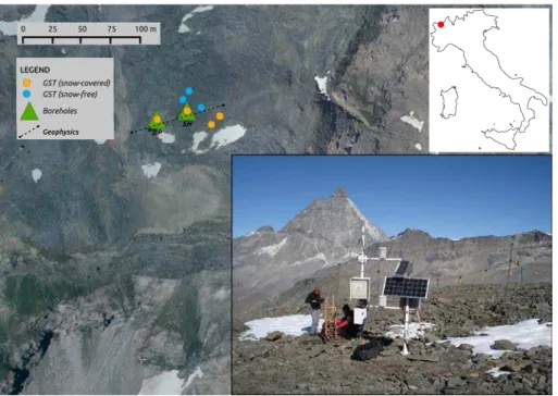
The Cime Bianche monitoring site (CB) is located in the western Alps at the head of the Valtournenche Valley (Valle d’Aosta, Italia, 45◦55′N–7◦41′E) on the Italian side of the Matterhorn, at 3100 m a.s.l. (Fig. 1). The site is located on a small plateau slightly westward degrading characterized by terraccettes, convexities and depressions that result in a high spatial variability of snow cover thickness during winter.

20

The bedrock lithology is homogeneous, mainly consisting of garnetiferous micas-chists and calcsmicas-chists belonging to the upper part of the Zermatt–Saas ophiolite com-plex (Dal Piaz, 1992). The bedrock surface is highly weathered and fractured, locally resulting in a cover of coarse-debris deposits with a thickness ranging from few cen-timeters to a couple of meters. The presence of small landforms like gelifluction lobes 25

(6)

diame-TCD

8, 4033–4074, 2014

variability

P. Pogliotti et al.

Title Page

Tables Figures

◭ ◮

Back Close

Full Screen / Esc

Discussion

P

a

per

|

Discus

sion

P

a

per

|

Discussion

P

a

per

|

Discussion

P

a

per

|

ters ranging between 0.6 to 3.4 m) suggests the potential presence of permafrost and cryotic phenomena.

The climate of the area is slightly continental. The long-term mean annual

precipi-tation is reported to be about 1000 mm year−1for the period 1931–1996 (Mercalli and

Cat Berro, 2003) while the in-situ records show a mean of 1200 mm year−1 _{for the}

5

period 2010–2013. The mean annual air temperature (MAAT) is about₋3.2◦C (mean

1951–2011). Mean monthly air temperatures are positive from June to September while February and July are respectively the coldest and the warmest months. The site is very windy and mainly influenced by NE–NW air masses. The wind action strongly contributes to the high spatial variability of snow cover thickness.

10

Permafrost research in the area started in the late 1990s (Guglielmin and Vannuzzo, 1995) with repeated campaigns of BTS (Bottom Temperature of Snow) measures and glaciological observations showing that the monitoring site was probably ice-covered during the climax of the Little Ice Age. In 2003, as a preliminary investigations for site selection, the potential permafrost occurrence in the area was assessed using 15

results from BTS, VES (Vertical Electrical Soundings) and ERT (Electrical Resistivity Tomography) and the application of numerical models like Permakart (Keller, 1992) and Permaclim (Guglielmin et al., 2003). Results of this preliminary analysis (unpublished) revealed that the area is characterized by the presence of discontinuous permafrost.

2.2 Instrumentation

20

(7)

TCD

8, 4033–4074, 2014

variability

P. Pogliotti et al.

Title Page

Tables Figures

◭ ◮

Back Close

Full Screen / Esc

Discussion

P

a

per

|

Discus

sion

P

a

per

|

Discussion

P

a

per

|

Discussion

P

a

per

|

2.2.1 Boreholes

A deep (DP) and a shallow (SH) borehole, reaching a depth of 41 and 6 m respec-tively, located about 30 m apart (Fig. 1), have been drilled in 2004 with core-destruction method. Both boreholes are 127 mm in diameter with a 60 mm sealed PVC pipe for sensor housing. The boreholes are equipped with thermistor chains based on resistors 5

type YSI 44031 (resolution 0.01◦C, absolute accuracy_±0.05◦C and relative accuracy

±0.02◦C). Sensors depths in meters from the surface are 0.02, 0.3, 0.6, 1, 1.6, 2, 2.3,

2.6, 3, 3.3, 3.6, 4, 4.6, 5.9 for SH and 0.02, 0.3, 0.6, 1, 1.6, 2, 2.6, 3, 3.6, 4, 6, 8, 10, 12, 14, 15, 16, 17, 18, 20, 25, 30, 35, 40, 41 for DP. In each borehole, the shal-lower sensors (0.02 and 0.3 m) are cabled on two independent chains and are used 10

to measure the ground surface temperature (GST) outside the PVC tube in order to avoid the thermal disturbance of the casing. Temperatures are sampled every 10 min and recorded by a Campbell Scientific CR800 datalogger. The system is equipped with a GPRS module for daily remote data transmission.

2.2.2 Ground surface temperature grid (GSTgrid)

15

A small grid (40 m_×10 m) is used for monitoring the spatial variability of GST (Ground Surface Temperature). The grid consists of 5 nodes, 4 at the corners and 1 in the center (Fig. 1). Each node is equipped with 2 platinum resistors PT1000 (resolution 0.01◦_C,

accuracy _±0.05◦C) buried in the ground at depths of 0.02 and 0.3 m (according to

Guglielmin, 2006). Ground temperatures are recorded hourly by a Geoprecision D-20

Log12 datalogger.

For the analysis, also the GST measured at the two boreholes are included, thus 7 nodes are overall considered. Ground surface at each node is mainly characterized by coarse-debris with a fine matrix of coarse-sand and fine-gravel. At each node, the sen-sors are placed in the matrix thus local ground conditions are nearly homogeneous be-25

(8)

TCD

8, 4033–4074, 2014

variability

P. Pogliotti et al.

Title Page

Tables Figures

◭ ◮

Back Close

Full Screen / Esc

Discussion

P

a

per

|

Discus

sion

P

a

per

|

Discussion

P

a

per

|

Discussion

P

a

per

|

the set is divided in snow-free and snow-covered nodes. The first group includes 3

nodes characterized by shallow or intermittent winter snow cover while the latter group includes 4 nodes that clearly show a long lasting deep snow cover with a damping of temperature oscillations during winter (Fig. 1).

2.2.3 Automatic weather station

5

An automatic weather station (AWS) is installed just above the borehole SH since 2006. Air temperature and relative humidity, atmospheric pressure, wind speed and direction, incoming and outgoing short- and long-wave solar radiation and snow depth are recorded every 10 min by a Campbell Scientific CR3000 datalogger. The system is equipped with a GPRS module for the daily remote data transmission. Since Septem-10

ber 2011 a second snow depth sensor has been installed in the surroundings of the DP borehole. Finally solid and liquid precipitations are measured since January 2009 by an OTT Pluvio2system.

2.3 Data analysis

This section reports a short description of the criteria applied for the calculation of the 15

synthesis parameters used in this study.

MAGT is the mean annual ground temperature at a specific depth (m) (e.g. MAGT₁₀). MAGST is the mean annual ground surface temperature. It is calculated with the sensors at 0.02 m or 0.3 m of depth (specified each time).

ALT is the active layer thickness defined as the maximum depth (m) reached by the 20

0◦C isotherm at the end of the warm season. It is calculated considering the maximum daily temperature at each sensor depth and interpolating between the deepest sen-sor with positive value and the sensen-sor beneath. The maximum of the resulting vector and the corresponding day are named ALT and ALTday respectively. Such procedure is applied on the warmest period (in depth) of the year, here fixed from 1 August to 25

(9)

TCD

8, 4033–4074, 2014

variability

P. Pogliotti et al.

Title Page

Tables Figures

◭ ◮

Back Close

Full Screen / Esc

Discussion

P

a

per

|

Discus

sion

P

a

per

|

Discussion

P

a

per

|

Discussion

P

a

per

|

TTOP is the MAGT at the top of the permafrost table (Smith and Riseborough, 1996). It is calculated by interpolation of the MAGT at depth of the ALT that is considering the first sensors just above and the first just below the ALT.

THO is the thermal offset within the active layer and is computed as TTOP-MAGST

(Burn and Smith, 1988). 5

ZAA is the depth beneath which there is almost no annual fluctuation in ground tem-perature, nominally smaller than 0.1◦C (van Everdingen, 2005). The annual fluctuation

(AF) is calculated at each sensor depth as the di_fference between annual maximum

and annual minimum of the mean daily temperatures. The ZAA is calculated by

inter-polation between the deepest sensor with AF greater than 0.1◦C and the sensor

be-10

neath. On deep nodes time series (below 8 m), a moving average window of 360 days is applied on hourly data before the daily aggregation to remove the electrical sensor’s noise (sometimes present).

All the synthesis parameters listed above, with the exception of ALT, are computed considering as reference period the hydrological year (beginning 1 October). All the 15

analysis are performed with the free statistical software R (R Core Team, 2014). When appropriate, the variability of the results is expressed in terms of standard error (se=

sd/√nwhere se is standard error, sd is standard deviation andnis the sample size).

2.4 Trend analysis

In order to look for linear trends that might reflect warming, two non-parametric meth-20

ods are applied to boreholes temperatures: Mann–Kendall test (MK) (Mann, 1945; Kendall, 1948) and Sen’s slope estimator (SS) (Sen, 1968). These methods are com-monly used to assess trends and related significance levels in hydro-meteorological time series such as water quality, stream flow, temperature and precipitation (e.g., Go-cic and Trajkovic, 2013; Kousari et al., 2013). The reason for using non-parametric 25

(10)

TCD

8, 4033–4074, 2014

variability

P. Pogliotti et al.

Title Page

Tables Figures

◭ ◮

Back Close

Full Screen / Esc

Discussion

P

a

per

|

Discus

sion

P

a

per

|

Discussion

P

a

per

|

Discussion

P

a

per

|

The procedure chosen includes (i) a pre-whiten of the data for removing the lag-1 autocorrelation components as recommended by von Storch and Navarra (1999) (see also Hamed, 2009), (ii) fitting of the trend’s slope with SS and (iii) testing of trend’s

sig-nificance level (p value) with MK. Such a procedure is implemented in the R-package

zyp (Bronaugh et al., 2013). 5

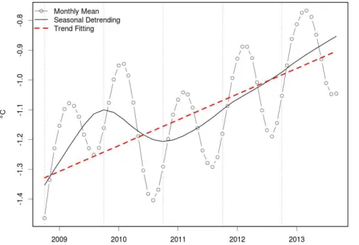
Given the short climatological time-span of the given borehole’s observations, a sea-sonal detrending is recommended, as suggested by Helsel and Hirsch (1992), for better discerning the long-term linear trend over time. Thus a seasonal decomposition based on loess smoother (Cleveland, 1979; Cleveland et al., 1990) is applied on the monthly aggregated time series of each borehole before applying SS and MK (Fig. 2). Such 10

a seasonal detrending method is implemented by the R-function stl (R Core Team,

2014).

2.5 Geophysics

At the end of the summer 2013, two geophysical surveys took place at the Cime Bianche with the objective to assess the composition of the subsurface. A first explo-15

rative geoelectric (ERT) profile was performed on 16 August 2013, and on 9 October 2013 the ERT measurement was repeated in combination with one refraction seismic tomography (RST) along the same line (see Fig. 1). Combining refraction seismic and ERT measurements enables to unambiguously identify the subsurface materials in the ground. Due to very different specific resistivities, ERT is best suited to differentiate 20

between ice and water whereas the distinction between air and ice can more easily

be accomplished by RST, because of large contrasts between their respectivepwave

velocities.

2.5.1 Electrical Resistivity Tomography (ERT)

A 94 m long electrode array composed of 48 electrodes with 2 m spacing was installed 25

(11)

TCD

8, 4033–4074, 2014

variability

P. Pogliotti et al.

Title Page

Tables Figures

◭ ◮

Back Close

Full Screen / Esc

Discussion

P

a

per

|

Discus

sion

P

a

per

|

Discussion

P

a

per

|

Discussion

P

a

per

|

was injected using varying electrode pairs, and the resulting potential differences were automatically measured by a Syscal (Iris Instruments) for each quadrupole possible with the Wenner–Schlumberger configuration (529 measurements, 23 depth levels). The electrode locations were marked with spray paint and a number of electrodes were left on site to facilitate further measurements.

5

The measured apparent resistivity datasets were then inverted using the RES2DINV software (Geotomosoft, 2014) with the following set-up. A robust inversion constraint was applied to avoid unrealistic smoothing of the calculated specific resistivities. Addi-tionally the depth of the model layers was increased by a factor 1.5 and an extended model was used to match the model grid of the corresponding seismic inversion. Note, 10

that for geometric reasons, the two lower corners of the resulting tomograms have very low sensitivity to the obtained data and should not be over-interpreted. Finally, a time-lapse inversion scheme was applied to the two ERT data sets yielding the percentage of resistivity change from the first measurements to the second. Here, an unconstraint inversion was chosen, meaning that the ERT measurements were inverted indepen-15

dently.

2.5.2 Refraction Seismic Tomography (RST)

The measurements were conducted using a Geode seismometer (Geometrics) and 24 geophones placed with 4 m spacing. A seismic signal was generated in-between every second geophone pair by repeatedly hitting a steel plate with a sledge hammer. To 20

improve the signal-to-noise ratio the signal was stacked at least 15 times at each lo-cation. Two additional o_ffset shot points were measured (3 m before the first geophone and 6 m beyond the last one) in order to maximize the spatial resolution and match the ERT profile length and depth of investigation.

The first arrivals of the seismic pwave were manually picked for each seismogram

25

using the software REFLEXW (Sandmeier, 2014). A Simultaneous Iterative Recon-struction Technique (SIRT) algorithm was then used to reconstruct a 2-D tomogram of

(12)

syn-TCD

8, 4033–4074, 2014

variability

P. Pogliotti et al.

Title Page

Tables Figures

◭ ◮

Back Close

Full Screen / Esc

Discussion

P

a

per

|

Discus

sion

P

a

per

|

Discussion

P

a

per

|

Discussion

P

a

per

|

thetic model the travel times are calculated and compared to the measured ones. The model is then updated iteratively by minimizing the residuals between measured and calculated travel times.

3 Results

3.1 Ground surface temperatures

5

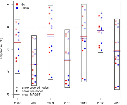
Figure 3 shows MAGST at 2 and 30 cm of depth for each hydrological year calculated on the seven GST nodes. The analysis of the GST dataset shows a mean range of the spatial variability of 2.5_±0.15◦_{C versus a mean range of the inter-annual variability of}

1.6_±0.12◦C. Some years (e.g. 2009, 2011, 2013) show a MAGST spatial variability

that can be greater than 3◦_{C, far exceeding the observed mean inter-annual variability.}

10

The time series analysis of snow-covered nodes (Schmid et al., 2012) reveals that the mean duration of the insulating snow cover is about 270 days while on snow-free nodes such effect is only sporadic or absent (not shown). On average the thermal offset

due to snow cover is about 1.5_±0.17◦_{C with snow covered nodes usually warmer than}

snow-free nodes. These observations confirm that the warming and cooling effects of

15

respectively a thick and thin snow cover (Zhang, 2005; Pogliotti, 2010) can coexist over short distances (<50 m) and lead to high spatial variability of the GST.

The results are similar at both depth. The difference between MAGST measured at

2 cm and 30 cm is, on average, 0.4_±0.11◦C with deeper sensors usually warmer than

the shallower ones. 20

3.2 Active layer

(13)

TCD

8, 4033–4074, 2014

variability

P. Pogliotti et al.

Title Page

Tables Figures

◭ ◮

Back Close

Full Screen / Esc

Discussion

P

a

per

|

Discus

sion

P

a

per

|

Discussion

P

a

per

|

Discussion

P

a

per

|

in Table 1). Missing values (column %NA) in both boreholes are lower than 4 % in all years.

ALT is the variable showing the greater difference between the two boreholes with a mean of 2.75_±0.35 m in SH and 4.78_±0.26 m in DP. The mean inter-annual diff

er-ence of ALT between the two boreholes is 2.03_±0.12 m while the mean absolute

inter-5

annual variability of ALT at borehole level is 1_±0.13 m. In both boreholes the maximum ALT has been recorded in 2012 while the minimum in 2010. ALT-Day is normally antic-ipated in DP (except 2013) with di_fferences ranging from few days (e.g. 2009) to more than 3 weeks (e.g. 2012). The MAGST is on average slightly lower in SH which nor-mally shows a thinner winter snow cover compared to DP (Fig. 4). The TTOP values 10

are very similar, around₋0.9◦_{C. The THO is negative in both boreholes (except 2013)}

with a mean value of about₋0.5◦C in DP and₋0.3◦C in SH.

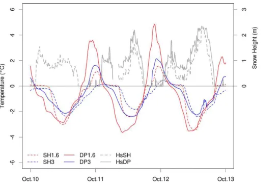
The values of Table 1 show that all the active layer variables are very similar between the two boreholes with the only exception of ALT which in DP is nearly double than in SH. To better understand the causes of this di_fference, the daily mean temperatures at 15

selected depths within the active layer of both boreholes and the corresponding snow cover thickness are compared in Fig. 4. Despite a consistently thinner snow depth is

recorded on SH compared to DP (mean di_fference_∼41_±14 cm during the winter

sea-sons 2012 and 2013), the duration of the insulating snow cover is similar (250_±16 days for SH vs. 254_±17 days for DP) and effectively does not determine a big difference in 20

MAGST (Table 1). Consequently the snow cover regimes above the two boreholes can be considered equivalent and snow probably plays a major role for the inter-annual variability of ALT while the observed spatial differences must be explained otherwise.

For these reasons we hypothesize that ALT di_fference may be related to a greater

ice/water content in SH compared to DP. This is also revealed by the geophysical sur-25

vey (see Sect. 3.4 and Fig. 7) and can be inferred by temperature at greater depth.

At 1.6 m (red lines, Fig. 4) a pronounced zero-curtain e_ffect can be observed in SH

(14)

TCD

8, 4033–4074, 2014

variability

P. Pogliotti et al.

Title Page

Tables Figures

◭ ◮

Back Close

Full Screen / Esc

Discussion

P

a

per

|

Discus

sion

P

a

per

|

Discussion

P

a

per

|

Discussion

P

a

per

|

zero-curtain reflects a large consumption of energy, both for ice melting during sum-mer and water freezing during winter resulting in lower temperatures of SH. Deeper down, the summer heat wave in SH is further delayed if compared to DP: at 3 m in SH (dashed blue lines) the zero-curtain effect is almost continuous from late-summer to early-winter (e.g. in 2010 and 2011) and it is not possible to see a breaking point 5

between melting and freezing processes. Such a behavior is totally missing in DP. It is also interesting to observe that freezing zero-curtain ends nearly contemporary at 1.6 and 3 m and is followed by a rapid temperature drop.

In conclusion, the ALT at Cime Bianche shows a pronounced spatial variability prob-ably caused by the variability of ice/water content in the sub-surface and associated 10

energy consumption resulting from freezing and melting processes.

3.3 Permafrost temperature and warming trend

Due to the small depth reached by the borehole SH, the analysis of deep temperature and permafrost temperature is limited to the borehole DP. Looking at temperature pro-files with depth (Fig. 5), the permafrost layer at Cime Bianche has a thickness greater 15

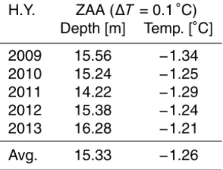
than 40 m and a mean temperature of about₋1.2◦C. The ZAA varies across years and

during the observation period ranged from a minimum of 14.2 m in 2011 to a maximum of 16.2 m in 2013 (Table 2). During the observed years, both minimum (solid lines) and maximum (dashed lines) temperature profiles (deeper than 8 m) tend to progressively shift toward warmer temperatures (Fig. 5). The only exceptions are represented by the 20

2011’s maximum and the 2009’s minimum, the latter only above 10 m of depth.

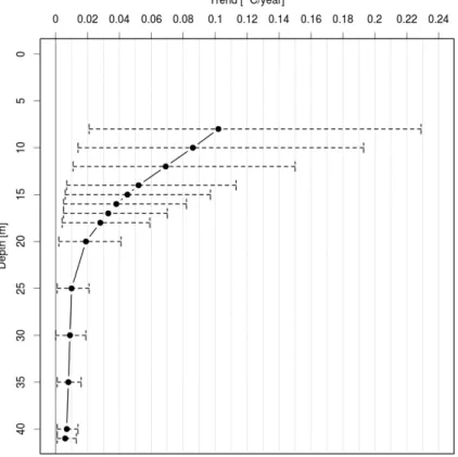
The observed temperature shift is also quantitatively supported by the trend analysis performed on deeper sensors (range 8–41 m of depth, Fig. 6). The analysis has been conducted at all depths within both boreholes but only trends below 8 m have shown to be significant (Kendall’sp value of the time series<0.01) hence only DP borehole 25

is shown. Figure 6 reveals that a pronounced warming rate is present at all depths although it exponentially decrease with depth, varying from around 0.1◦_{C year}−1_{at 8 m}

(15)

TCD

8, 4033–4074, 2014

variability

P. Pogliotti et al.

Title Page

Tables Figures

◭ ◮

Back Close

Full Screen / Esc

Discussion

P

a

per

|

Discus

sion

P

a

per

|

Discussion

P

a

per

|

Discussion

P

a

per

|

systematically unbalanced toward higher values and the lower boundaries are always above zero. This means that, at all depths, the statistical distribution of all possible fitted trends is asymmetric towards greater values and also that negative significant trend have never been fitted by the model.

Based on the trend analysis, is possible to conclude that permafrost at Cime Bianche 5

is degrading with a warming rate decreasing with depth.

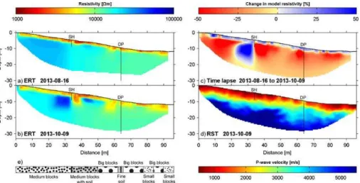
Figure 7 shows the final distribution of specific resistivity for the two ERT measure-ments, the percentage of change in the model resistivity between the two time steps

and the p wave velocity distribution over the same subsection. Additionally, the

sur-10

face characteristics and a detailed analysis of the geophysical properties at the two borehole locations (SH and DP, Fig. 8) are included in the analysis.

The overall characteristics of both ERT profiles are very similar (Fig. 7a and b) and can be divided into three main zones: a low resistive layer directly below the surface varying between 2.5 m thickness at the top of the slope to 7 m thickness at the bottom, 15

respectively, two high resistive areas with values exceeding 20 000Ωm located below

the superficial layer (from the start of the subsection to the superficial borehole, 0–34 m and between 40–52 m) and a less high resistive area on the lower part of the profile below 5 m depth.

Comparing the two ERT data sets (cf. also the time-lapse image in Fig. 7c), one can 20

observe a clear increase of the uppermost low resistive layer between August and Oc-tober which is coherent with a thickening of the active layer observed in the borehole

temperature during this period. Another main di_fference between the two

measure-ments is the apparition of two low resistive zones at 34 m and 60 m visible down to 10 m and 15 m depth, respectively. These areas can also be seen in the ERT tomo-25

(16)

TCD

8, 4033–4074, 2014

variability

P. Pogliotti et al.

Title Page

Tables Figures

◭ ◮

Back Close

Full Screen / Esc

Discussion

P

a

per

|

Discus

sion

P

a

per

|

Discussion

P

a

per

|

Discussion

P

a

per

|

These changes are clearly visible in blue (increase) and red (decrease) colors in Fig. 7c. As said before the two datasets were inverted independently within the time-lapse scheme. A constrained inversion (results not shown here) would yield very sim-ilar overall distribution of resistivity changes the only difference being a much smaller range of values. The large area of resistivity increase located just above the superficial 5

borehole location and reaching down to the bottom of the profile corresponds to the displacement of the high resistive area observed in the ERT tomograms.

The RST tomogram exhibits much less lateral variations than the ERT results (see Fig. 7d), pointing to the influence of liquid water in the ERT results. One can clearly

see a relatively slow layer with velocities between 300 and 1500 m s−1 (red and dark

10

red colors) just below the surface with varying thickness between 3 and 5 m. This layer is thickest in the vicinity of the shallow borehole (SH) and thinnest at DP (64 m). Be-low this first layer the velocities increase steadily until reaching the maximum (around 6400 m s−1_{). The rate of velocity increase is strongest around 40 m and there is a clear}

distinction between the upper part of the profile (until 45 m) and the lower one. At depth 15

the high velocity zone is present in the upper part and not in the lower part of the profile. Conversely the velocities at the surface are much higher in the lower part (especially around DP) than in the upper part.

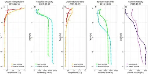
Both geophysical profiles show clear differences in the subsurface properties at the boreholes locations. To relate in detail the results yielded by the geophysics and the 20

measured temperature, the vertical distribution of specific resistivity, seismic velocity and ground temperature at SH and DP are shown in Fig. 8.

4 Discussion

4.1 Ground surface temperatures

In this study both the inter-annual and the spatial variability of MAGST within a re-25

(17)

TCD

8, 4033–4074, 2014

variability

P. Pogliotti et al.

Title Page

Tables Figures

◭ ◮

Back Close

Full Screen / Esc

Discussion

P

a

per

|

Discus

sion

P

a

per

|

Discussion

P

a

per

|

Discussion

P

a

per

|

Bianche, the mean range of spatial variability (2.5_±0.15◦_{C) far exceeds the mean}

range of observed inter-annual variability (1.6_±0.12◦_{C). Given the comparatively}

ho-mogeneous characteristics of the ground surface at the sensors’ locations, such a vari-ability is essentially caused by the heterogeneity of the snow cover thickness both in space (e_ffect of wind redistribution and micro-morphology) and time (e_ffect of variable 5

weather conditions and precipitations).

The thermal effect of snow cover on ground surface temperature has been

exten-sively analyzed (e.g., Goodrich, 1982; Keller and Gubler, 1993; Zhang, 2005; Luetschg et al., 2008). In recent years, with the advances of mini-loggers technology, the number of field experiments aimed at the characterization of the spatial variability of GST has 10

grown. Recently Gubler et al. (2011) observed a spatial variability of more than 2.5◦_C

within a number of square homogeneous areas of 10 m_×10 m. In Norway, Isaksen et al.

(2011) report that MAGST varied by 1.5–3.0◦_{C over distances of 30–100 m in a region}

characterized by mountain permafrost. Rödder and Kneisel (2012) observed ranges exceeding 4.3◦C between adjacent loggers (<50 m), although this values include in-15

homogeneities of surface characteristics. Similar results were obtained by Gisnås et al. (2014) who observed a variability of the MAGST of up to 6◦_{C within heterogeneous}

ar-eas of 0.5 km2.

The inter-annual variability of MAGST caused by snow is also well known and doc-umented by a number of studies (Romanovsky et al., 2003; Hoelzle et al., 2003; 20

Karunaratne and Burn, 2004; Brenning et al., 2005; Etzelmüller, 2007; Ødegård and Isaksen, 2008; Schneider et al., 2012) but rarely has been explicitly analyzed and quan-tified. An exception in the Alps is represented by Hoelzle et al. (2003) who reported an inter-annual variability of_±2.7◦C measured during two seasons on 8 mini-loggers with differing surface characteristics in the Murtèl–Corvatsch area. Our results thus report 25

a more robust quantification of the mean inter-annual GST variability (1.6_±0.12◦_C),

based on a longer time series (7 years).

The obtained results are very similar at both measurement depth. Given such a small

(18)

TCD

8, 4033–4074, 2014

variability

P. Pogliotti et al.

Title Page

Tables Figures

◭ ◮

Back Close

Full Screen / Esc

Discussion

P

a

per

|

Discus

sion

P

a

per

|

Discussion

P

a

per

|

Discussion

P

a

per

|

arguable that to describe the spatial variability of GST and run long-term GST obser-vations, measures at two or more depth are not needed.

4.2 Active layer

In this study both thaw depth and temperature fluctuations within the active layer of two adjacent boreholes have been compared. Such experimental design provides direct 5

evidence of the small-scale spatial variability of the ALT and allow to compare the effect of snow cover and ice/water content on sub-surface temperatures.

From 2009 to 2013 the ALT at Cime Bianche varied within 2 and 5.5 m with a mean

inter-annual variability of 1_±0.13 m. These ranges of thaw depth are comparable to

those recorded in other alpine sites (PERMOS, 2013) and the same is true for the 10

observed inter-annual variability (Anisimov et al., 2002; Christiansen, 2004; Schneider et al., 2012; Smith et al., 2010).

ALT in the borehole SH is systematically lower than in DP (mean difference 2.03_± 0.15 m) even though all the active layer parameters (MAGST, TTOP, THO see Table 1) are very similar between the two boreholes. On one side such a similarity suggests 15

that snow cover regimes above the two boreholes are nearly equivalent thus snow probably plays a major role just for the inter-annual variability of ALT. On the other side the pronounced spatial variability of ALT is probably caused by the variability of ice/water content in the sub-surface and associated variation of energy consumption resulting from freezing and melting processes. Probably snowmelt and meltwater in-20

filtration along preferential discontinuities (a borehole acts a discontinuity itself) is dif-ferent between SH and DP. Hilbich et al. (2008) observed at Schilthorn (Swiss Alps) a similar situation between two boreholes 15 m apart, ascribing the lower ALT of one borehole to the higher moisture contents (and related freezing) caused by preferential water flow paths from the surrounding slopes. Schneider et al. (2012) analyzed the 25

(19)

TCD

8, 4033–4074, 2014

variability

P. Pogliotti et al.

Title Page

Tables Figures

◭ ◮

Back Close

Full Screen / Esc

Discussion

P

a

per

|

Discus

sion

P

a

per

|

Discussion

P

a

per

|

Discussion

P

a

per

|

The different amount of available water in the active layer of the two boreholes is also reflected by the occurrence of the zero-curtain in the borehole SH and its absence in the borehole DP. In the upper part of the active layer a pronounced zero-curtain can be observed two times per year, (i) from snow melt to mid-summer (spring zero-curtain) and (ii) from the snow onset to mid-winter (autumn zero-curtain). Recently Zenklusen 5

Mutter and Phillips (2012) deeply analyzed similar behaviors on a sample of 10 bore-holes in Switzerland observing that, on average, the duration of the spring zero-curtain is usually shorter than the autumn one and is strongly dependent on snow depth at the end of the winter. At Cime Bianche, in the deeper part of the active layer such a distinc-tion between spring and autumn zero-curtain is not always possible. As observed also 10

by Rist and Phillips (2005) it may happen that, below a certain depth, the ground tem-perature does not become positive because the energy from the summer heat wave is not sufficient to melt all ice before the onset of the subsequent winter season. This con-tinuous zero-curtain is more probable when an higher amount of meltwater is available (Scherler et al., 2010; Kane et al., 2001) and can occur at di_ffering depth from year to 15

year strongly influencing the resulting ALT.

4.3 Permafrost temperature and warming trend

In order to look for trends that might reflect warming, two non-parametric methods have been applied to boreholes temperatures time series. The detected linear trends are statistically significant (Kendall’spvalue<0.01) only at depth below 8 m and span 20

the range 0.1–0.01◦_{C year}−1_{decreasing exponentially with depth. The latter evidence}

suggests that at Cime Bianche the permafrost is warming from surface.

As discussed also by Zenklusen Mutter et al. (2010), the detection of trends on time series covering a short time-span needs caution and adoption of specific criteria. Moreover the estimation of uncertainties and significance levels are also fundamen-25

(20)

TCD

8, 4033–4074, 2014

variability

P. Pogliotti et al.

Title Page

Tables Figures

◭ ◮

Back Close

Full Screen / Esc

Discussion

P

a

per

|

Discus

sion

P

a

per

|

Discussion

P

a

per

|

Discussion

P

a

per

|

Permafrost warming trends have been observed worldwide, both at high latitudes (Harris, 2003; Osterkamp, 2005; Smith et al., 2005; Osterkamp, 2007; Isaksen et al., 2007; Farbrot et al., 2013; Jonsell et al., 2013) and at lower latitudes in high mountain (Vonder Mühll, 2001; Harris, 2003; Gruber, 2004; Wu and Zhang, 2008; Phillips and Mutter, 2009; Zenklusen Mutter et al., 2010; PERMOS, 2013; Haeberli, 2013).

5

Recently in the Alps Zenklusen Mutter et al. (2010) detected linear trends applying generalized least-square methods on daily temperature time series of two boreholes in the Muot da Barba Peider ridge (Eastern Swiss Alps). For the deep frozen bedrock be-tween 8 and 17.5 m a general warming trend was found, with significant (pvalue<0.05) values ranging respectively from 0.042 to 0.025◦C year−1. At Cime Bianche a similar 10

range of warming rate exists between 16 and 20 m. The substantial difference

be-tween the two sites is that the Swiss boreholes are drilled at the top of a NW-oriented ridge with a mean slope of 38◦ thus with a strong 3-D thermal effect induced by to-pography (Noetzli et al., 2007). In the mountains of Scandinavia Isaksen et al. (2007) reports linear warming trends between 20 and 60 m of depth ranging from about 0.05 15

to 0.005◦C year−1 respectively over three sites while Isaksen et al. (2011) found an increase in mean ground temperature between 6 and 9 m of depth at two sites, with rates ranging from about 0.015 to 0.095◦_{C year}−1_{. Recently at Tarfala mountain station}

(Sweden) Jonsell et al. (2013) found linear trends over 11 years (2001–2011) ranging from 0.047 to 0.002◦_{C year}−1_{between 20 and 100 m of depth respectively.}

20

The absolute values of warming rates are di_fficult to compare because of di_ffering site characteristics, differing geographical regions and differing methods used for trend’s detection. Nevertheless, some similitudes exist between our and the above mentioned case studies: (i) trends are di_fficult to detect at shallower depth because of the higher seasonal variability of temperatures (ii) warming trends are mainly significant below 8– 25

(21)

TCD

8, 4033–4074, 2014

variability

P. Pogliotti et al.

Title Page

Tables Figures

◭ ◮

Back Close

Full Screen / Esc

Discussion

P

a

per

|

Discus

sion

P

a

per

|

Discussion

P

a

per

|

Discussion

P

a

per

|

Given the relatively high resistivity andP wave velocities along the profiles, the pres-ence of permafrost observed in the borehole data is confirmed by the geophysics over the whole profile length (Fig. 7). Moreover a clear discrepancy between the upper part of the profile, where SH is located, and the lower one with borehole DP can be seen in 5

both, the ERT and the RST data.

At DP the P wave velocities indicates the presence of weathered bedrock close to

the surface whereas at SH a layer of coarse-debris deposits in the uppermost 5 m is

confirmed by very low P wave velocities. Conversely, P wave velocities at depth are

higher for SH (_∼6000 m s−1_{) than for DP (}

∼5000 m s−1, see also Fig. 8). This diff

er-10

ence, also seen in the resistivity data (around 17 000_Ωm at SH and 13 000_Ωm at DP), would indicate that a larger ice content is present in the upslope part of the profile than in the lower part. This is in good agreement with the spatial variation of ALT highlighted in Sect. 3.2 and the zero curtain phase observed only at SH (see Fig. 4).

The low resistivity and low velocity layer near the surface, which thickness increases 15

visibly between August and October in the ERT data, is considered to be the active layer. Figure 8 compares the vertical distribution of specific electrical resistivity,P wave velocity and temperature for both boreholes and dates. On the first glance, there seems to be a mismatch between resistivity and temperature regarding ALT for SH. However, in SH borehole temperatures in August show constant values at the freezing point 20

between 1 and 3 m depth (between 2 and 4 m in October), the deeper level being the depth of the sharply increasing resistivity values. As resistivity is sensitive to the liquid water content its values will not increase significantly before most of this liquid water has been frozen, coinciding with a temperature increase to values below the freezing point (e.g., Hauck, 2002). Due to the higher water/ice content in SH, this phenomena 25

(_∼vertical zero-curtain) is only seen in SH and not in DP.

(22)

TCD

8, 4033–4074, 2014

variability

P. Pogliotti et al.

Title Page

Tables Figures

◭ ◮

Back Close

Full Screen / Esc

Discussion

P

a

per

|

Discus

sion

P

a

per

|

Discussion

P

a

per

|

Discussion

P

a

per

|

and temperature data are due to very different surface and subsurface properties. The general description of the surface constitution (Fig. 7e) is already an indication of these differences: DP is located in-between two zones with big blocks (from pluri-decimetric to metric), whereas SH is located at the junction between medium size blocks (from pluri-centimetric to decimetric) mixed and non-mixed with soil. These di_fferences in 5

subsurface material are likely to cause the strong differences in P wave velocities at the two borehole locations.

The two low resistive areas (34–40 m and 53–60 m) visible already in August and more pronounced on the second ERT profile in October are interpreted as preferential water flow path. Since the melt water cannot infiltrate through the two ice-rich (high 10

resistive) bodies close by (at 20–33 and 40–52 m horizontal distance), it is forced to follow a preferential path in between. The lower infiltration area is constrained in the upper part by the ice rich zone and in the lower one by the presence of bedrock near the surface.

Finally the displacement of the high resistive area observed near SH (blue zone at 15

depth on the time-lapse tomogram) is most likely an inversion artefact (overcompensa-tion) due to the appearance of the low resistive area in the second ERT profile.

5 Conclusions

This paper presents a first synthesis on the thermal state and recent evolution of per-mafrost in the monitoring site of Cime Bianche. The analysis has been focused on: the 20

spatial and temporal variability of MAGST, the small scale (20–40 m) spatial variability of ALT and the warming rate of deep permafrost temperatures.

The analysis of MAGST has been conducted considering seven years of monitoring on 7 sensors located in nearly homogeneous conditions in terms of both topographic and ground surface characteristics. Such experimental design allowed to quantify the 25

(23)

sys-TCD

8, 4033–4074, 2014

variability

P. Pogliotti et al.

Title Page

Tables Figures

◭ ◮

Back Close

Full Screen / Esc

Discussion

P

a

per

|

Discus

sion

P

a

per

|

Discussion

P

a

per

|

Discussion

P

a

per

|

tematically colder than those with a long lasting deep snow cover; (ii) the snow cover variability alone can leads to a spatial variability of MAGST greater than its inter-annual variability.

The analysis of ALT spatial variability has been conducted within two adjacent bore-holes considering 6 years of observations as well as by the analysis of ERT and seismic 5

profiles. The results show that ALT at Cime Bianche has a pronounced spatial

variabil-ity caused by a different ice/water content in the sub-surface while the snow cover

probably plays a role just in the inter-annual variability of ALT.

The warming rates of ground temperatures time series below 8 m of depth have been analyzed by two non-parametric methods considering 5 years of monthly data. 10

The results show that permafrost at Cime Bianche is degrading with a warming rate which is higher at 8 m depth and exponentially decreasing with depth. Detected trends are similar to those observed recently in others boreholes both in the Alps and northern mountain environments. Moreover a review of the existing literature reveals a number of similitudes between our findings and the existing studies.

15

The Supplement related to this article is available online at doi:10.5194/tcd-8-4033-2014-supplement.

Acknowledgements. The authors are grateful to the lifts company Cervino S.p.a for their con-tinuous logistical support to the research activities at the site of Cime Bianche.

C. Pellet and C. Hauck gratefully acknowledge a grant from the Swiss National Science

20

Foundation (project SOMOMOUNT No. 200021_143325).

References

Allen, S. K. and Huggel, C.: Extremely warm temperatures as a potential cause of recent high mountain rockfall, Global Planet. Change, 107, 59–69, doi:10.1016/j.gloplacha.2013.04.007, 2013. 4034

(24)

TCD

8, 4033–4074, 2014

variability

P. Pogliotti et al.

Title Page

Tables Figures

◭ ◮

Back Close

Full Screen / Esc

Discussion

P

a

per

|

Discus

sion

P

a

per

|

Discussion

P

a

per

|

Discussion

P

a

per

|

Anisimov, O., Shiklomanov, N., and Nelson, F.: Variability of seasonal thaw depth in permafrost regions: a stochastic modeling approach, Ecol. Model., 153, 217–227, doi:10.1016/S0304-3800(02)00016-9, 2002. 4036, 4050

Beltrami, H.: Climate from borehole data: Energy fluxes and temperatures since 1500, Geo-phys. Res. Lett., 29, 2111, doi:10.1029/2002GL015702, 2002. 4036

5

Bence, J. R.: Analysis of short time series: correcting for autocorrelation, Ecology, 76, 628–639, 1995. 4037

Bommer, C., Phillips, M., and Arenson, L. U.: Practical recommendations for planning, con-structing and maintaining infrastructure in mountain Permafrost, Permafrost Periglac., 21, 97–104, doi:10.1002/ppp.679, 2010. 4035, 4036

10

Brenning, A., Gruber, S., and Hoelzle, M.: Sampling and statistical analyses of BTS measure-ments, Permafrost Periglac., 16, 383–393, doi:10.1002/ppp.541, 2005. 4036, 4049

Bronaugh, D., Werner, A., and For the Pacific Climate Impacts Consortium: zyp: Zhang+ Yue-Pilon trends package, available at: http://cran.r-project.org/package=zyp (last access: July 2014), 2013. 4042

15

Burn, C. and Smith, C.: Observations of the “Thermal Offset” in near-surface mean annual ground temperatures at several sites near Mayo, Yukon Territory, Canada, Arctic, 41, 99– 104, doi:10.14430/arctic1700, 1988. 4041

Christiansen, H. H.: Meteorological control on interannual spatial and temporal variations in snow cover and ground thawing in two northeast Greenlandic

Circumpolar-Active-Layer-20

Monitoring(CALM) sites, Permafrost Periglac., 15, 155–169, doi:10.1002/ppp.489, 2004. 4050

Christiansen, H. H., Etzelmüller, B., Isaksen, K., Juliussen, H., Farbrot, H., Humlum, O., Jo-hansson, M., Ingeman-Nielsen, T., Kristensen, L., Hjort, J., and Others, A.: The thermal state of permafrost in the nordic area during the international polar year 2007–2009, Permafrost

25

Periglac., 21, 156–181, doi:10.1002/ppp.687, 2010. 4035

Cleveland, R., Cleveland, W., McRae, J. E., and Terpenning, I.: STL: A seasonal-trend decom-position procedure based on loess, Journal of Official Statistics, 6, 3–73, 1990. 4042 Cleveland, W.: Robust locally weighted regression and smoothing scatterplots, J. Am. Stat.

Assoc., 74, 829–836, doi:10.1080/01621459.1979.10481038, 1979. 4042

30

(25)

TCD

8, 4033–4074, 2014

variability

P. Pogliotti et al.

Title Page

Tables Figures

◭ ◮

Back Close

Full Screen / Esc

Discussion

P

a

per

|

Discus

sion

P

a

per

|

Discussion

P

a

per

|

Discussion

P

a

per

|

permafrost evidence for the European Alps", The Cryosphere, 5, 651–657, doi:10.5194/tc-5-651-2011, 2011. 4035

Dal Piaz, G. V.: Le Alpi dal M. Bianco al Lago Maggiore: 13 Itinerari Automobilistici e 97 Escur-sioni a Piedi, Vol. 1, Seven Hills Books, Padova, Italy, 1992. 4037

DeConto, R. M., Galeotti, S., Pagani, M., Tracy, D., Schaefer, K., Zhang, T., Pollard, D., and

5

Beerling, D. J.: Past extreme warming events linked to massive carbon release from thawing permafrost, Nature, 484, 87–91, doi:10.1038/nature10929, 2012. 4034

Etzelmüller, B.: The regional distribution of mountain permafrost in Iceland, Permafrost Periglac., 199, 185–199, doi:10.1002/ppp.583, 2007. 4049

Etzelmüller, B.: Recent advances in mountain permafrost research, Permafrost Periglac., 24,

10

99–107, doi:10.1002/ppp.1772, 2013. 4035

Farbrot, H., Isaksen, K., Etzelmüller, B., and Gisnås, K.: Ground thermal regime and permafrost distribution under a changing climate in Northern Norway, Permafrost Periglac., 24, 20–38, doi:10.1002/ppp.1763, 2013. 4052

Fischer, L., Purves, R. S., Huggel, C., Noetzli, J., and Haeberli, W.: On the influence of

to-15

pographic, geological and cryospheric factors on rock avalanches and rockfalls in high-mountain areas, Nat. Hazards Earth Syst. Sci., 12, 241–254, doi:10.5194/nhess-12-241-2012, 2012. 4034, 4036

Fischer, L., Huggel, C., Kääb, A., and Haeberli, W.: Slope failures and erosion rates on a glacierized high-mountain face under climatic changes, Earth Surf. Proc. Land., 38, 836–

20

846, doi:10.1002/esp.3355, 2013. 4034

Geotomosoft: Res2dinv software Tutorial: 2-D and 3-D electrical imaging surveys, available at: www.geotomosoft.com (last access: July 2014), 2014. 4043

Gisnås, K., Westermann, S., Schuler, T. V., Litherland, T., Isaksen, K., Boike, J., and Et-zelmüller, B.: A statistical approach to represent small-scale variability of permafrost

tem-25

peratures due to snow cover, The Cryosphere Discuss., 8, 509–536, doi:10.5194/tcd-8-509-2014, 2014. 4049

Gocic, M. and Trajkovic, S.: Analysis of changes in meteorological variables using Mann– Kendall and Sen’s slope estimator statistical tests in Serbia, Global Planet. Change, 100, 172–182, doi:10.1016/j.gloplacha.2012.10.014, 2013. 4041

30

(26)

TCD

8, 4033–4074, 2014

variability

P. Pogliotti et al.

Title Page

Tables Figures

◭ ◮

Back Close

Full Screen / Esc

Discussion

P

a

per

|

Discus

sion

P

a

per

|

Discussion

P

a

per

|

Discussion

P

a

per

|

Gruber, S.: Permafrost thaw and destabilization of Alpine rock walls in the hot summer of 2003, Geophys. Res. Lett., 31, L13504, doi:10.1029/2004GL020051, 2004. 4035, 4052

Gruber, S. and Haeberli, W.: Permafrost in steep bedrock slopes and its temperature re-lated destabilization following climate change, J. Geophys. Res.-Earth, 112, F02S18, doi:10.1029/2006JF000547, 2007. 4035

5

Gruber, S. and Haeberli, W.: Mountain permafrost, in: Permafrost Soils, 33–44, doi:10.1007/978-3-540-69371-0, Innsbruck, Austria/Springer, 2009. 4035, 4036

Gruber, S. and Hoelzle, M.: The cooling effect of coarse blocks revisited: a modeling study of a purely conductive mechanism, in: Proceedings of the 9th International Conference on Permafrost, 557–561, 29 June–3 July 2008, Fairbanks, Alaska, USA, 2008. 4036

10

Gruber, S., King, L., Kohl, T., Herz, T., Haeberli, W., and Hoelzle, M.: Interpretation of geother-mal profiles perturbed by topography: the alpine permafrost boreholes at Stockhorn Plateau, Switzerland, Permafrost Periglac., 15, 349–357, doi:10.1002/ppp.503, 2004. 4036

Gubler, S., Fiddes, J., Keller, M., and Gruber, S.: Scale-dependent measurement and analy-sis of ground surface temperature variability in alpine terrain, The Cryosphere, 5, 431–443,

15

doi:10.5194/tc-5-431-2011, 2011. 4036, 4049

Guglielmin, M.: Ground surface temperature (GST), active layer and permafrost monitoring in continental Antarctica, Permafrost Periglac., 17, 133–143, doi:10.1002/ppp.553, 2006. 4039 Guglielmin, M. and Cannone, N.: A permafrost warming in a cooling Antarctica?, Climatic

Change, 111, 177–195, doi:10.1007/s10584-011-0137-2, 2012. 4035

20

Guglielmin, M. and Vannuzzo, C.: Studio della distribuzione del permafrost e delle relazioni con i ghiacciai della piccola età glaciale nell’alta valtournenche (Valle d’Aosta, Italia), Atti Ticinesi di Scienze della Terra, 38, 119–127, 1995. 4038

Guglielmin, M., Aldighieri, B., and Testa, B.: PERMACLIM: a model for the distribution of mountain permafrost, based on climatic observations, Geomorphology, 51, 245–257,

25

doi:10.1016/S0169-555X(02)00221-0, 2003. 4035, 4038

Guglielmin, M., Dalle Fratte, M., and Cannone, N.: Permafrost warming and vegetation changes in continental Antarctica, Environ. Res. Lett., 9, 045 001, doi:10.1088/1748-9326/9/4/045001, 2014a. 4035

Guglielmin, M., Worland, M. R., Baio, F., and Convey, P.: Permafrost and snow monitoring

30

(27)

TCD

8, 4033–4074, 2014

variability

P. Pogliotti et al.

Title Page

Tables Figures

◭ ◮

Back Close

Full Screen / Esc

Discussion

P

a

per

|

Discus

sion

P

a

per

|

Discussion

P

a

per

|

Discussion

P

a

per

|

Haeberli, W.: Mountain permafrost research frontiers and a special long-term challenge, Cold Reg. Sci. Technol., 96, 71–76, doi:10.1016/j.coldregions.2013.02.004, 2013. 4034, 4052 Haeberli, W., Noetzli, J., Arenson, L. U., Delaloye, R., Gärtner-Roer, I., Gruber, S.,

Isaksen, K., Kneisel, C., Krautblatter, M., and Phillips, M.: Mountain permafrost: de-velopment and challenges of a young research field, J. Glaciol., 56, 1043–1058,

5

doi:10.3189/002214311796406121, 2010. 4035

Hamed, K.: Enhancing the effectiveness of prewhitening in trend analysis of hydrologic data, J. Hydrol., 368, 143–155, doi:10.1016/j.jhydrol.2009.01.040, 2009. 4042

Harris, C.: Warming permafrost in European mountains, Global Planet. Change, 39, 215–225, doi:10.1016/j.gloplacha.2003.04.001, 2003. 4035, 4037, 4052

10

Harris, C. and Haeberli, W.: Permafrost monitoring in the high mountains of Europe: the PACE project in its global context, Permafrost Periglac., 11, 3–11, doi:10.1002/ppp.377, 2001. 4035 Harris, C., Arenson, L. U., Christiansen, H. H., Etzelmüller, B., Frauenfelder, R., Gruber, S., Haeberli, W., Hauck, C., Hölzle, M., Humlum, O., Isaksen, K., Kääb, A., Kern-Lütschg, M., Lehning, M., Matsuoka, N., Murton, J., Nötzli, J., Phillips, M., Ross, N., Seppälä, M.,

Spring-15

man, S., and Vonder Mühll, D.: Permafrost and climate in Europe: monitoring and mod-elling thermal, geomorphological and geotechnical responses, Earth-Sci. Rev., 92, 117–171, doi:10.1016/j.earscirev.2008.12.002, 2009. 4035

Hauck, C.: Frozen ground monitoring using DC resistivity tomography, Geophys. Res. Lett., 29, 12-1–12-4, doi:10.1029/2002GL014995, 2002. 4053

20

Helsel, D. R. and Hirsch, R. M.: Trend analysis, in: Statistical Methods in Water Resources, chap. 12, Amsterdam, Holland/Elsevier, 1992. 4037, 4042

Hilbich, C., Hauck, C., Hoelzle, M., Scherler, M., Schudel, L., Völksch, I., Vonder Mühll, D., and Mäusbacher, R.: Monitoring mountain permafrost evolution using electrical resistivity tomog-raphy: a 7-year study of seasonal, annual, and long-term variations at Schilthorn, Swiss Alps,

25

J. Geophys. Res., 113, F01S90, doi:10.1029/2007JF000799, 2008. 4035, 4050

Hipp, T., Etzelmüller, B., and Westermann, S.: Permafrost in Alpine Rock faces from Jotunheimen and Hurrungane, Southern Norway, Permafrost Periglac., 25, 1–13, doi:10.1002/ppp.1799, 2014. 4035

Hoelzle, M., Haeberli, W., and Stocker-Mittaz, C.: Miniature ground temperature data

log-30