Application of OSN in membrane cascade for purification of the API Amoxicillin

(1)

Licenciatura em Ciências da Engenharia Química e Bioquímica

Application of OSN in membrane cascade

for purification of the API Amoxicillin

Dissertação para obtenção do Grau de Mestre em

Engenharia Química e Bioquímica

Orientadores:

Professor Andrew G. Livingston (IC)

Doutora Ludmila Peeva (IC)

Co-orientador:

Professora Isabel Coelhoso (FCT-UNL)

Júri:

Presidente: Prof. Doutora Ana Maria Martelo Ramos Arguente: Prof. Doutor João Paulo Serejo Goulão Crespo Vogal: Prof. Doutora Isabel Maria Rola Coelhoso

(2)

(3)

Application of OSN in membrane cascade for

purification of the API Amoxicillin

Dissertação para obtenção do Grau de Mestre em

Engenharia Química e Bioquímica

Orientadores:

Professor Andrew G. Livingston (IC)

Doutora Ludmila Peeva (IC)

Co-orientador:

Professora Isabel Coelhoso (FCT-UNL)

IMPERIAL COLLEGE LONDON

Faculty of Engineering

Department of Chemical Engineering and Chemical Technology

UNIVERSIDADE NOVA DE LISBOA

Faculdade de Ciências e tecnologia

Departamento de Química

(4)

(5)

Copyright Susana Cristina Dias Ramos Ferreira, FCT-UNL, UNL

(6)

(7)

research group and provide me this amazing experience.

To my coordinator Ludmila Peeva for the guidance, support, help, attention and availability. I appreciate the comfort she gave me with any questions and uncertainties.

I am deeply grateful to João Burgal, my daily supervisor, who helped me through the whole project, including writing this thesis. Thank you for all the caring, support, joy, good mood and friendship with which you received me every day.

To my colleagues/friends Carlos Gomes, Irina Valtcheva, James Campbell, Shanta Kumar, Ana Gil, Pedro Bastos, Jeong Kim and Joana Guedes that supported me in every step of the way and made my days much brighter and fun inside and out of the university.

I would also like to thank all the other members of the Separation Engineering and Technology research group for their support during my stay at Imperial College.

To Professor Isabel Coelhoso for being always available to help with any questions and showing interest in my work.

To my parents and sister that made this amazing journey possible and were always there to support, encourage, understand and help me when I most needed.

I would like to thank to Karta, Fateh, Denise and Lockram that received me with open arms and made me feel at home.

I also would like to thank all my friends for their emotional support, encouragement and friendship even being far away from them.

(8)

(9)

Massachusetts Institute of Technology (MIT) had the objective of purifying the API amoxicillin containing an initial concentration of 30ppm of the compound 4-hydroxy-l-phenylglycine (impurity) using an OSN membrane cascade.

Project proposal:

 Solubility and stability studies of the API in different solvents.  Solvent choice for the separation process.

 Dissociation study of the API and impurity to exploit a promising optimization of the process.

 Membrane screening using dead-end and m-CSTR upside-down measurements.  Process modeling and simulation of different configurations

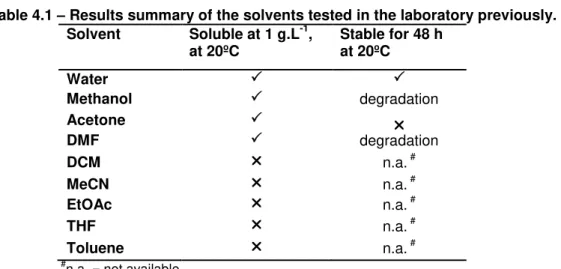
Amoxicillin showed to be a sensitive compound to work with having a low solubility and a fast decomposition in the studied solvents. The solvents tested in detail were water, acetone, ethanol and methanol, being water the one choose to performed the purification.

From the dissociation study it was possible to understand the possible exploitation of the pH parameter in the optimization of the separation process.

In the membrane screening the effect of pressure and pH were studied in six types of membranes. It could be conclude that the main obstacle for the purification process was the membrane performance itself, with insufficient separation between the compounds (difference of 10 p.p. in rejection). The most promising results were obtained using the TFNF-DL membrane, with an API rejection of 99.12% and an impurity rejection of 87.80%.

The process modelling was performed in a semi-batch mode with one and two stages, respectively, and in continuous mode with two-stages and two different configurations. An increase from two to three stages was also analyzed for the continuous configuration II. A maximum purity of 99.65% with a yield of 97.86% was obtained with the semi-batch two-stage cascade system. From the continuous three stage cascade system, a purity of 98.65% and a yield of 98.54% were achieved.

(10)

(11)

RESUMO

O presente projecto desenvolvido na Universidade Imperial de Londres (ICL) em colaboração com Instituto de Tecnologia de Massachussets (MIT) tinha como objectivo a purificação do API amoxicilina partindo de uma concentração inicial do composto 4-hydroxy-l-phenylglycine (impureza) de 30 ppm recorrendo a nanofiltração com solventes orgânicos numa cascada de membrana.

Proposta de trabalho:

 Estudos de solubilidade e estabilidade do API em diferentes solventes.  Escolha do solvente mais conveniente para à purificação.

 Estudo da dissociação de ambos os compostos para explorar uma possível optimização do processo.

 Testes de diafiltrações a diferentes membranas utilizando dead-end e m-CSTR.  Modelação e simulação do processo considerando diferentes configurações.

A amoxicilina demonstrou ser um composto de difícil solubilidade e fácil decomposição. Os solventes testados em detalhe foram água, acetona, etanol e metanol, sendo água o solvente escolhido para proceder à purificação.

O estudo da dissociação iónica dos compostos demostrou a possível optimização do processo de separação através da exploração do parâmetro pH.

Na realização dos testes de diafiltração, o efeito da pressão e do pH foram estudados em seis tipos de membranas. Conclui-se que o principal obstáculo do processo de purificação seria o desempenho da própria membrana, pelo facto de nao efectuar uma separaracao eficiente entre os dois compostos (diferença de 10 p.p. entre rejeições). O resultado mais promissor foi obtido com a membrana TFNF-DL, tendo uma rejeição do API de 99.12% e uma rejeição da impureza de 87.80%.

A modelação do processo foi realizada a um sistema semi-continuo contendo uma única e duas etapas de separação; e ainda a duas configurações diferentes de um sistema em continuo com duas etapas de separação. Um aumento do número de duas para três etapas foi também analisado para a configuração II em contínuo. Uma pureza de 99.65% com um rendimento de 97.86% foi obtida usando o sistema semi-continuo com duas etapas de separação. Através do sistema de três etapas em contínuo, foi possível alcançar uma pureza de 98.65% com um rendimento de 98.54%.

(12)

(13)

LIST OF FIGURES

Figure 1.1 – Schematic diagrams of the principal types of membranes (Adapted from Baker,

2004)……….3

Figure 1.2 –Typical rejection curves for membranes with a sharp cut-off and a diffuse cut-off

(Adapted from Mulder, 1996)………6

Figure 1.3 –Schematic representation of the two transport mechanisms through membranes: (A) the pore-flow model and (B) the solution-diffusion model (Adapted from Baker, 2004)..……6

Figure 1.4 – Concentration polarization: concentration profile under steady-state conditions

(Adapted from Baker, 2004)………..8

Figure 1.5–Effect of fouling and concentration polarization on flux (Adapted from Mulder,

1996)……….9

Figure 1.6 –Typical pharmaceutical batch operation (Adapted from Dunn, Wells and Williams,

2010)………..11

Figure 1.7 – Schematic representation of membrane filtration system design: a) dead-end, b)

cross-flow mode (Adapted from Arunima Saxena, 2009)……….14

Figure 1.8 – General representation of the modules and units in a membrane cascade: P-permeate; R- retentate; y – number of stages; n, p and z -number of membrane units in the first,

second and y stage, respectively (Adapted from Siew et all, 2013)………....15

Figure 1.9 – Modes of cascade operation: A) simple symmetric cascade; B) symmetric countercurrent recycle cascade (Adapted from Siew et all, 2013)………..16

Figure 2.1 –Molecular representation of the studied compounds: A) Amoxicillin; B)

4-hydroxy-L-phenylglycine……….21

Figure 2.2 - Kinetically controlled synthesis of amoxicillin using penicillin G acylase as catalyst.

(Adapted from Alemzadeh, 2010)………..22

Figure 3.1 - Schematic of experimental pressure cell used for membrane screening. (Adapted

from Scarpello & Livingston, 2002)………...30

Figure 3.2 –Layout of the membrane separator cell (m-CSTR). Legend: 1 – Inlet/outlet ports; 2 – Feed/retentate chamber; 3 – Inner o-ring; 4 – Membrane; 5 –Sintered plate; 6 – Outer o-ring;

7 –Cover. (Adapted from Peeva & Livingston , 2013)………...31

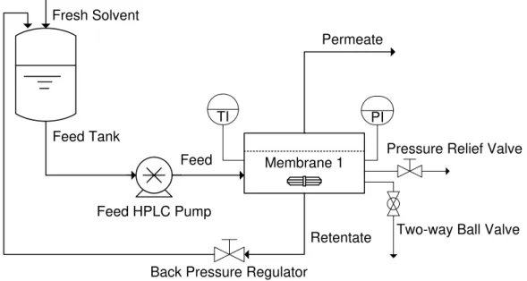
Figure 3.3 - Process diagram of the single membrane system (PI: Pressure gauge; TI:

Temperature indicator)……….32

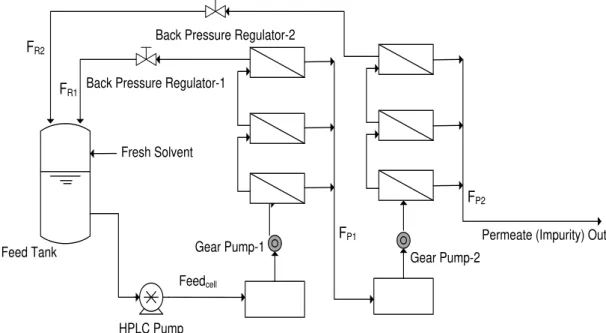
Figure 3.4 - Scheme of the two-stage cascade with the main equipment and streams highlighted. Legend: Feedcell– Feed flow-rate to the first stage; FR1 – Retentate flow-rate from stage 1; FP1 – Permeate flow-rate from stage 1; FP2 – Permeate flow-rate from stage 2; FR2 –

Retentate flow-rate from stage 2………36

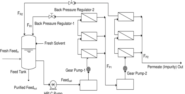
Figure 3.5 - Scheme of the continuous two-stage cascade with the main equipment and streams highlighted. Legend: Feedin– Feed flow-rate in (to be purified); Feedout– Feed flow-rate out (purified); Feedcell– Feed flow-rate to the first stage; FR1– Retentate flow-rate from stage 1; FP1– Permeate flow-rate from stage 1; FP2– Permeate flow-rate from stage 2; FR2– Retentate

(16)

– –

out (purified); Feedcell– Feed flow-rate to the first stage; FR1– Retentate flow-rate from stage 1; FP1– Permeate flow-rate from stage 1; FP2– Permeate flow-rate from stage 2; FR2– Retentate

flow-rate from stage 2………..38

Figure 3.7 - Scheme of the continuous two-stage cascade with the main equipment and streams highlighted. Legend: Feedin– Feed flow-rate in (to be purified); Feedout– Feed flow-rate out (purified); Feedcell– Feed flow-rate to the first stage; FR1– Retentate flow-rate from stage 1; FP1– Permeate flow-rate from stage 1; FP2– Permeate flow-rate from stage 2; FR2– Retentate flow-rate from stage 2; FP3 – Permeate flow-rate from stage 3; FR3– Retentate flow-rate from

stage 3………39

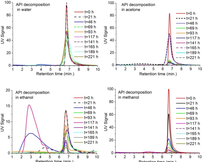
Figure 4.1 – UV signal, from the HPLC analysis, of the samples taken over time for each solution. Solutions prepared with 1g.L-1of amoxicillin in the different solvents………..44

Figure 4.2 - Concentration of amoxicillin over time in the different solvents. Solutions prepared with 1 g.L-1 of amoxicillin. These results represent an average of two experiments and the error

bars are the standard deviation of the mean………45

Figure 4.3 – Isoelectric point determination: A) Titration curve of amoxicillin a T=20ºC. Experimental conditions: CAPI= 1.32 mmol.L

-1

; CNaOH= 49.65 mmol.L -1

; Viniz. = 10 mL; B) Titration curve of 4-hydroxy-L-phenylglycine a T=20ºC. Experimental conditions: CAPI= 1.43 mmol.L

-1 ; CNaOH= 49.65 mmol.L

-1

; Viniz. = 10 mL; C) Molecular structure and ionizable groups from amoxicillin; D) Molecular structure of 4-hydroxy-L-phenylglycine……….46

Figure 4.4 - Dissociation profiles of the amoxicillin and 4-hydroxy-L-phenylglycine, considering

100% molar percentage in the beginning (see appendix III for

calculations)………...47

Figure 4.5 - Process diagram of the single membrane system (PI: Pressure gauge; TI:

Temperature indicator)……….53

Figure 4.6 – HPLC UV signal from the mixture compounds in 1 g.L-1 aqueous solution: A) amoxicillin (90.0% pure); B) 4-hidroxy-L-phenylglycine (99.0% pure). The red points indicate the different peak areas and the label values the retention times of those

peaks………..57

Figure 4.7 - HPLC UV signal results from the powder analysis. A) powder from TFNF-DL- C membrane trial at 0.7 g.L-1; B) powder from TFNF-DL- D membrane trial at 0.9 g.L-1; C) powder from TFNF-DL- E membrane trial at 1 g.L-1. The red points indicate the different peak areas and the label values the retention times of those peaks. The peaks without red points are the ones

with dispersible areas (≤ 2)……….58

Figure 4.8 – Concentration profile for the API in the membrane interface, Cim, as a function of the mass transfer coefficient. Profiles for the experimental trial using the TFNF-DL – E for both pH conditions considering a retentate API concentration of 2.74 mol.m-3 (1 g.L-1) and a solvent rejection of 1%...59

Figure 4.9 – Single-stage semi-batch system: A) Mass profiles over filtration time for both compounds in the retentate stream; B) Yield and purity profiles for the API,

amoxicillin………..62

Figure 5.1 – Two-stage semi-batch system considering an effective pressure in the second stage of 25 bar and a Rc = 0.17: A) Total normalized mass profiles over filtration time for both compounds in the retentate stream; B) Yield and purity profiles for the API, amoxicillin, , and the

correspondent zoom.………...63

Figure 5.2 – Modeled effect of recycle ratio, Rc, on the API yield and purity of amoxicillin in a

(17)

using MATLAB®, considering a ΔP1 of 30 bar and varying the feed flow rate (Feed

effective pressure of the second stage (ΔP2) parameters. A permeability of 2.14 L.m-2

.h-1.bar, an API rejection of 99.12% and an impurity rejection of 87.80% were used based on the

TNFN-DL-E membrane trials.……….65

Figure 5.4 –Purity and yield profiles of the API in the purified outlet stream (Feedout) obtained by MATLAB®, considering a ΔP1 of 30 bar and varying the feed flow rate (Feedin) and the

effective pressure of the second stage (ΔP2) parameters. A permeability of 2.14 L.m-2.h-1.bar,

an API rejection of 99.12% and an impurity rejection of 87.80% were used based on the

TNFN-DL-E membrane trials………..66

Figure 5.5 – Purity (figure A) and yield (figure B) profiles of the API in the purified outlet stream (Feedout) obtained using MATLAB®, considering a ΔP1 of 30 bar and varying the feed flow rate (Feedin) and the effective pressure of the second stage (ΔP2) parameters. A permeability of 2.14 L.m-2.h-1.bar, an API rejection of 99.12% and an impurity rejection of 87.80% were used

based on the TNFN-DL-E membrane trials.……….67

Figure 5.6 – Concentrations in the purified stream over time (h) obtained using MATLAB®: A)

API profile; B) Impurity profile Parameters considered: ΔP1= 30 bar; ΔP2= 25 bar; Feedin =

0.343 L.m-2.h-1 and a permeability of 2.14 L.m-2.h-1.bar. The recycle ratio and the feed utilization of the systems are respectively Rc= 0.17 and FU= 7.90 (vide Table 5.1)……….68

Figure 5.7 – Profiles of the API purity and yield obtained using MATLAB®. Parameters

considered: ΔP1= 30 bar; ΔP2= 25bar; Feedin = 0.343 L.m

-2

.h-1 and a permeability of 2.14 L.m -2

.h-1.bar. The recycle ratio and the feed utilization of the systems are respectively Rc= 0.17 and

FU= 7.90 (vide Table 4.9)…...………..………..69

Figure 5.8 – Concentration profile of the API in the Feedout obtained using MATLAB®,

considering a ΔP1 of 30 bar and varying the Feedinand ΔP2 parameters. A permeability of 2.14

L.m-2.h-1.bar, an API rejection of 99.12% and an impurity rejection of 87.80% were

considered.………70

Figure 5.9 – Purity (figure A) and yield (figure B) profiles of the API in the purified out stream

(Feedout) obtained using MATLAB®, considering a ΔP1 of 30 bar and varying the feed flow rate

(Feedin) and the effective pressure of the second stage (ΔP2) parameters. A permeability of 2.14 L.m-2.h-1.bar, an API rejection of 99.12% and an impurity rejection of 87.80% were used

based on the TNFN-DL-E membrane trials.……….71

Figure 6.1 – Behavior of the feed utilization (FU) and recycle ratio (Rc) with the difference of

effective pressure between the two stages (ΔP1-ΔP2) obtained using MATLAB®. A ΔP1 of 30

bar, permeability of 2.14 L.m-2.h-1.bar, an API rejection of 99.12% and an impurity rejection of 87.80% were considered.………...72

Figure 6.2 – Concentrations in the purified stream over time (h) obtained using MATLAB®: A) API profile; B) Impurity profile. Parameters considered: ΔP1= 30 bar; ΔP2= 5 bar; Feedin = 0.343 L.m-2.h-1 and a permeability of 2.14 L.m-2.h-1.bar. The recycle ratio and the feed utilization of the systems are respectively Rc= 0.17 and FU= 7.90 (vide Table 5.2)………..73

Figure 6.3 – Profiles of the API purity and yield obtained using MATLAB®. Parameters

considered: ΔP1= 30 bar; ΔP2= 5 bar; Feedin = 0.343 L.m

-2

.h-1 and a permeability of 2.14 L.m -2

.h-1.bar. The recycle ratio and the feed utilization of the systems are respectively Rc= 0.17 and

(18)

(19)

LIST OF TABLES

Table 1.1 – Classification of membrane processes according to their driving forces (Adapted

from Mulder, 1996)……….4

Table 1.2 – Comparison of various pressure driven membrane processes. (Adapted from

Coulston Vol.2, 2002)………5

Table 3.1 - Amoxicillin and 4-hydroxy-l-phenylglycine relevant properties. (Data obtain from Sigma-Aldrich safety data sheets; Foulstone, 1982; O’Neil, 2001; VSDB and the chemical book

via online)………...27

Table 3.2 –Summary of the membrane tested in this work………..29

Table 4.1 –Results summary of the solvents tested in the laboratory previously……….43

Table 4.2. - Comparison of the results obtained for the amoxicillin solubility. Solutions prepared

with 10g.L-1of amoxicillin in the different solvents………..43

Table 4.3 - Summary of the screening results conducted using water as solvent with a pressure

of 10 bar and a temperature of 22ºC……….49

Table 4.6 - Summary of the screening results conducted using water as solvent at 22º………52

Table 4.7 - Summary of the screening results conducted using water as solvent at 20 bar at 22ºC. Pure solvent average flux is 52.5± 2.5 L.m-2.h-1………...54

Table 4.8 - Summary of the screening results conducted using water as solvent at 20 and 30 bar at 22ºC. Pure solvent average flux is 160.7± 0.1 L.m-2.h-1 at 20bar and 225.0± 15.2 L.m-2.h-1

at 30 bar……….56

Table 4.9 - Summary of the parameters considerations based on the semi-batch experimental

trial using the TFNF-DL-E membrane………...61

Table 5.1 - Values for independent and dependent variables, obtained with MATLAB®, in order to optimize contions (considering a permeability of 2.14 L.m-2.h-1.bar, an API rejection of 99.12% and an impurity rejection of 87.80%). Boundary condition established: API maximum

concentration = 8 g.L-1………...68

Table 5.2 - Values for independent and dependent variables, obtained with MATLAB®, in order to optimize conditions (considering a permeability of 2.14 L.m-2.h-1.bar, an API rejection of 99.12% and an impurity rejection of 87.80%). Boundary condition established: API maximum concentration = 8 g.L-1………...73

Table 5.3 - Values for independent and dependent variables, obtained with MS Excel SolverTM, in order to optimize contions (considering a permeability of 2.14 L.m-2.h-1.bar, an API rejection of 99.12% and an impurity rejection of 87.80%). Boundary condition established: API maximum concentration = 8 g.L-1………...75

Table 5.4 - Comparison between the performances of the different systems configurations described previously. A permeability of 2.14 L.m-2.h-1.bar, an API rejection of 99.12% and an

(20)

(21)

ABREVIATIONS

API Active pharmaceutical ingredient

CP Concentration polarization

DCM Dichloromethane

DBB Dibromobutane

DBX Dibroxylene

DMAc N,N-dimetylacetamide

FU Feed utilization ratio

GTI Genotoxin impurity

HPLC High pressure liquid chromatography

HPGM P-hydroxyphenylglycine methyl ester

HVNC High value natural compounds

IPA Isopropanol

ISA Integrally skinned asymmetric membranes

m-CSTR Continuous single stirred tank reactor/membrane separator

MeCN Acetonitrile

MEK Methyl ethyl ketone

MF Microfiltration

MeOH Methanol

MW Molecular weight (g.mol-1)

MWCO Molecular weight cut-off

NF Nanofiltration

NRe Reynolds number

Nsh Sherwoods number

NSc Schmidts number

PEEK Poly(ether ether ketone)

PEG 400 Polyethylene glycol

PFR Flow reactor

PGA Enzyme penicillin G acylase

PI Polyimide

PP Polypropylene

Rc Rcycle ratio

RO Reverse osmosis

TFC Thin-film composite membranes

THF Tetrahydrofuran

UF Ultrafiltration

UV Ultraviolet

(22)

(23)

NOMENCLATURE

J Membrane flux (L.m-2.h-1)

R Rejection of the solute (%)

B Membrane permeability (L.m-2.h-1.bar)

C Concentration (g.L-1)

Cs,0 Solute concentration in the feed side (mol.m -3

) Cs,p Solute concentration in the permeate side (mol.m

-3 )

A Membrane area (m2)

rP Pore size

ε surface porosity (dimensionless)

Ʈ Pore tortuosity (dimensionless)

ƞ Solvent viscosity (kg.m-1.s-1)

l Membrane thikness

KL Solvent sorption

KS L

Solute distribution

D Fick’s law diffusion coefficient (m2.s-1)

R Gas constant (8.341 J.mol-1.K-1) k’ Mass transfer coefficient (m.s-1)

d Diameter (m)

D Diffusion coefficient (m2.s-1) w Radial speed of the stir (rad.s-1)

ρ Density (kg.m-3)

μ Viscosity (Pa.s)

VAPI API molal volume (cm 3

.mol-1)

ʋ Molar volume of the compound (m3.mol-1)

F Flow rate (L.h-1)

Feed cell Feed into the first stage Feedin Fresh feed into the feed tank Feedout Purified feed out of the feed tank

Rc Recycle ratio

FU Feed utilization

t Time (h)

T Temperature (°C / K )

V Volume (L)

P Pressure (bar/Pa)

SUBSCRIPTS

i Solute

R Retentate stream

P Permeate stream

FM Feed side liquid phase at the membrane liquid interface

b Bulk

m Membrane surface

v Volume

(24)

(25)

CHAPTER I

(26)

(27)

1.1 Membrane Technology

Membranes have gained an important place in chemical technology and are used in a broad range of applications. This emerging technology has the potential to be applied in diversified industries such as the medical, pharmaceutical, wastewater, petrochemical and food.

A membrane is defined as a selective barrier between two phases which restricts the transport of some substances and allows the transport of others from one phase to another (Mulder, 1996). This transport trough the membrane takes place as a result of a driving force, i.e. by pressure, temperature, concentration or electrical potential difference, acting on the components in the feed. In addition to steric exclusion membrane-solvent interactions, pressure, feed concentration, temperature and charge can influence the membrane performance and such factors can hence be used to fine tune the separation (Mulder, 1996; Screewathanawut et al., 2010; Baker 2004).

1.1.1 Membrane types

A membrane can be homogeneous or heterogeneous, symmetric or asymmetric in structure, solid or liquid in terms of state and can be charged or neutral.

Membranes can generally be classified into biological membranes, or synthetic membranes which can be either organic (polymeric or liquid) or inorganic (ceramic, metal or zeolite) (Mulder, 1996). Synthetic polymeric membranes are commonly classified according to their structure as symmetric or asymmetric. These two classes can be subdivided as shown in Figure 1.1.

Symmetrical Membranes

Porous membrane Dense membrane

(nonporous)

Asymmetrical Membranes

Integrally Skinned membrane Thin Film Composite membrane

Figure 1.1 – Schematic diagrams of the principal types of membranes (Adapted from Baker, 2004).

The porous membranes are usually used in filtration processes, where separation is made by particle size. Nonporous membranes are frequently used in pervaporation and gas separation processes where the separation occurs according to the difference in solubility and diffusivity of the molecules in the membrane material. When these membranes are charged, they mostly separate by exclusion of ions of the same charge as the fixed ions of the membrane structure

(28)

unlike symmetric membranes, high selectivity with high transport rates, which brings a great economical advantage (Mulder, 1996; Screewathanawut et al., 2010).

The toplayer and its porous sublayer may be formed in a single operation, with the formation of integrally skinned asymmetric membranes (ISA), or separately, with the formation of thin-film composite (TFC) membranes. In TFC membranes the skin-layer and the porous sublayer can be made of different materials, which mean that the active layer and porous sublayer can be independently optimized to maximize the overall membrane performance. Nevertheless, the skinned asymmetric membranes have considerably lower manufacturing costs comparing to the TFC membranes (Mulder, 1996; Screewathanawut et al., 2010).

The interest in membranes formed from less conventional materials has increased. Ceramic membranes for example are being applied in microfiltration and ultrafiltration fields do to their superior performance in terms of chemical and thermal stability relative to polymeric membranes. This main class of inorganic membranes do not deform under pressure nor do they swell and are easier to clean, (cleaning agents such as strong acids and alkali, can be used). Furthermore, they have a greater lifetime than that of organic polymeric membranes. However, they tend to be more expensive and brittle than polymeric membranes and are also less versatile in applications. In addition, their large-scale synthesis and module construction is not as easy as for polymeric membranes (Vandezande, Givers and Vankelecom, 2008). That is why the majority of membranes used commercially are still polymer-based (Mulder, 1996; Screewathanawut et al., 2010; Vandezande, Givers and Vankelecom, 2008)

1.1.2 Membrane Processes

Membrane processes can be classified according to their driving forces.

Table 1.1 – Classification of membrane processes according to their driving forces (Adapted from Mulder, 1996).

Pressure difference

Concentration difference

Temperature difference

Electrical potential difference

Microfiltration Pervaporation Thermo-osmosis Electrodialysis

Ultrafiltration Gas separation Membrane distillation Electro-osmosis

Nanofiltration Vapour permeation - Membrane electrolysis

Reverse Osmosis Dialysis - -

Piezodialysis Difusion dialysis - -

Carrier-mediated

transport - -

(29)

Table 1.2 – Comparison of various pressure driven membrane processes. (Adapted from Coulston Vol.2, 2002)

Microfiltration Ultrafiltration Nanofiltration and Reverse Osmosis

Particle separation

Pore sizes ≈ 0,05-10 μm

Macromolecules separation (bacteria, yeast)

Pore sizes ≈ 1-100 nm

Separation of low MW solutes (salts, glucose, lactose, micropollutents)

Pore sizes ˂ 2nm

Low pressure applied

(˂ 2 bar) Medium pressure applied (1-10 bar)

High pressure applied

(≈ 10-60 bar)

Separation based on the particle size

Separation based on differences in solubility and diffusivity

1.1.3 Membrane Characterization

Membranes can be characterized in terms of their performance and morphology. In terms of performance the most important parameters are flux, permeance, rejection, diffusion coefficients and separation factors. Morphological parameters include both physical (e.g. pore shape, pore size, pore distribution, membrane/top layer thickness, etc) and chemical parameters (e.g. charge, hydrophobicity, etc).

Performance parameters are dependent on morphological parameters, for instance pore size, shape and distribution have a big influence on the membrane flux. Depending on the pore size and shape the molecules will permeate easily or not (bigger pore sizes correspond to a better permeation and a higher flux) and if the pore distribution is uniform or not, membrane flux can be compromised due to fouling formation and pore blocking (non uniform pore distribution results in areas with higher flux than others promoting fouling in the less permeated areas). However, and despite the importance of characterizing and better understanding physical-chemical parameters, it is the functional parameters that from a practical perspective, determine the usefulness of the membrane (Mulherkar and Van Reis, 2004; Cuperus and Smolders, 1991).

The permeability rate, also denominated by flux, J (L.m-2.h-1), is defined as the volume of liquid permeating through the membrane (Vp) per unit of area (A) and time (t).

= VP_A.t

Equation I.1

Many parameters like temperature, pressure and solute concentration affect the flux of membranes. The permeate rate tend to increase with increasing temperature, because of reduction in solvent viscosity and increased polymer chain mobility (Van der Bruggen, Geens and Vandecasteele, 2002). An increase in pressure also led to an increase in flux. Solute concentration has an adverse effect on flux because of osmotic pressure and concentration polarization.

Membrane selectivity can be expressed using the rejection coefficient, Ri. This coefficient is defined as the ability of the membrane to separate a solute i from the feed solution and it is usually given by,

( ) (

)

Equation I.2

(30)

The selectivity can also be described by separation factor, α, when working with gas or organic solvent mixtures, being defined as the ratio between the coefficient of the concentrations of components A and B in the permeate, yA and yB, and the concentrations of the components in the retentate, xA and xB (Mulder, 1996).

Another important concept in the characterization of a membrane is the ‘molecular weight cut-

off’ (MWCO), which represents the minimum molecular weight (MW) that is 90 % rejected by a

membrane. This parameter, despite being useful as a starting point when screening for suitable membranes for a specific mixture separation, can be a poor estimation of the membrane performance. Pore size distribution, solvent environment, molecular shape, charge, functional groups, occurrence of polarization phenomena, temperature and the applied pressure are all factors that also affect the membrane rejection. (Mulder, 1996; Vandezande, Gevers and Vankelecom, 2008; See Toh et al., 2007; Yang et al., 2001).

NF and OSN membranes are characterized by a sigmoidal rejection curve, as the ones depicted in Figure 1.2, and they can discriminate molecules with molecular weight in the range of 200 to 2000 Da (Mulder, 1996; Vandezande, Gevers and Vankelecom, 2008).

Figure 1.2 – Typical rejection curves for membranes with a sharp cut-off and a diffuse cut-off (Adapted from Mulder, 1996).

1.1.4 Transport in membranes

In order to understand and possibly predict fluxes and rejections for a certain membrane, the transport mechanism of solutes and solvents through porous or dense films of different membranes should be thoroughly understood.

Three groups of mathematical models are used to describe the transport through membranes: irreversible thermodynamics models, pore-flow model and solution-diffusion model. The most reliable and commonly used transport models are the pore-flow and the solution-diffusion models. They describe, respectively, the transport through porous (e.g. micro and ultrafiltration membranes) and dense membranes (e.g. reverse osmosis, gas separation and pervaporation membranes).

(A) (B)

(31)

Pore-flow model

The pore-flow model assumes that different permeants are separated through tiny pores in the membrane by size-exclusion. This separation is accomplished by a pressure gradient across the membrane transporting the permeants through the pores. It is supposed that there are no concentration gradients, i.e. the solute and solvent concentration are constant over the membrane. Thus, the transport through porous membranes can be described based on hydrodynamic analysis by

Darcy’s law (Equation I.3) in which k is the permeability coefficient, that contains membrane structural

factors as membrane pore size (rp), surface porosity (ε), pore tortuosity (τ), solvent viscosity (η) and dP/dX is the pressure gradient over the membrane.

= k. dP_d= _8.η.τε.rp dP_d

Equation I.3 Solution-diffusion model

The solution-diffusion was initially used to explain transport of gases across polymeric film and nowadays it became the most widely accepted explanation of membrane transport. This model assumes that permeants dissolve in the membrane material and then dissolve through the membrane due to a concentration gradient, while the pressure within the membrane is constant at the highest level. The separation between different permeants occurs due to differences in their solubilities and diffusivities (Baker, 2004). Following the assumptions made, two simple equations could be derived for volume and solute flux:

v= D. _l.R.TL.C.v (ΔP Δ )= (ΔP Δ )

Equation I.4

s=Ds. s_l L (_{Cs,0 Cs,p})= _{(Cs,0 Cs,p)}

Equation I.5

where D and DS are the Fick’s law diffusion coefficients, K L

and KS L

are the solvent sorption and the solute distribution, respectively, C_{is the solvent concentration, v is the solvent molar flux,}l_{is the} membrane thickness, Cs,0 is the solute concentration in the feed side and Cs,p is the solute concentration in the permeate side; the constants Ba and B_s are known as the solvent and solute permeability, respectively (Baker, 2004).

OSN membranes are intermediate between truly porous and truly solution-diffusion membranes, and so they are best described by transient mechanisms that take into account the changing contributions of the diffusive and convective mechanisms, like the irreversible thermodynamics and the pore-flow models presented, or the solution-diffusion with imperfections model (Bhanushali et al., 2002),that accounts for the occurrence of convective flow and for the partial flux coupling effect. Plus, and since OSN membranes are applied to non-aqueous systems, special considerations regarding the various interactions between the system components and membrane swelling are also needed (Bhanushali et al., 2002; Boam and Nozari, 2006; Dijkstra Bach and Ebert., 2006; Robinson et al., 2004).

1.1.5 Strengths and drawbacks in membrane processes

(32)

Membrane processes still have some limitations, that particularly slow down large-scale applications (Baker, 2004; Vandezande, Gevers and Vankelecom, 2008). The most relevant limitations are discussed in the following sub-sections. A special attention was given to problems related to pressure driven membrane processes, like NF and OSN.

1.1.5.1 Concentration Polarization

Concentration polarization (CP) is the accumulation of solutes at the membrane active layer surface as a result of a permeate flow through the membrane. It creates a higher solute concentration at the membrane surface compared with bulk. This phenomenon has greater effects in pressure-driven processes due to high pressures used. In such processes CP leads to flux reduction due to increased pressure, that must be overcome, but also an increase in the driving force for the solute(s), reducing membrane selectivity. The increase in solute concentration at the membrane surface can also lead to a diffusive back flow towards the bulk of the feed, resulting in a concentration gradient between the bulk (Cs,b) and the membrane surface (Cm), creating a boundary layer which increases the resistance to mass transfer (Mulder, 1996).

In the boundary layer:

v.Cs DsdCs_dx = v.Cs,p

Figure 1.4 – Concentration polarization: concentration profile under steady-state conditions (Adapted from Baker, 2004).

It is possible to minimize the concentration polarization effect by decreasing the boundary layer thickness. This can be achieved by increasing the fluid flow velocity past the membrane surface, by using membrane spacers, or by using pulsating flow, as all these options increase turbulent mixing at the membrane surface (Mulder, 1996; Baker, 2004).

It is known that concentration polarization increases exponentially with the volume flux, Jv. That is why after a certain pressure, the flux does not increase further on increasing the pressure and the so called limiting flux, J∞, is achieved. Thus, there is no point in having super-high-flux

membranes, since the maximum flux will always be limited by osmotic pressure and concentration polarization. The only advantage of these membranes would be a reduction in energy costs, since they would allow for the same flux at lower applied pressure, minimize the overall processing time and limit the required membrane area (Mulder, 1996).

C

s,m

C

s,b

Bulk feed

C

s,p

Permeate flux

:

_Jv.Cs,p

Membrane

Boundary layer

(33)

1.1.5.2 Membrane fouling

Concentration polarization can result in membrane fouling, which is the deposition of retained solutes in the membrane, by adsorption, pore blocking, precipitation or cake formation. The type of separation problem and the type of membrane used in MF and UF make these processes the most susceptible to concentration polarization and fouling of all pressure driven membrane processes (Mulder, 1996). Fouling problems are, however, much more complex for NF processes, since the interactions leading to fouling take place at nanoscale, and are therefore difficult to understand (Van der Bruggen Mänttäri & Nyström., 2008).

One of the main consequences of membrane fouling is the decrease of flux. This has a negative impact on the operational costs of the process since the permeate production gets lower and/or higher trans-membrane pressures are required (Mulder, 1996).

Classical solutions to fouling are the pre-treatment of the feed and cleaning of membranes. Membrane design and process conditions can also be optimized to minimize fouling phenomena. Nevertheless, membrane modification is potentially the most sustainable solution, as it would allow to virtually avoid the problem (Mulder, 1996; Van der Bruggen Mänttäri & Nyström., 2008).

Figure 1.5 – Effect of fouling and concentration polarization on flux (Adapted from Mulder, 1996).

1.1.5.3 Insufficient separation

The incomplete separation is a major impediment for a wide application of membrane processes, including NF (Van der Bruggen Mänttäri & Nyström, 2008).

As mentioned before, membranes are characterized by a sigmoidal rejection curve which never is completely sharp. This will be translated in an insufficient separation between the different compounds on the basis of molecular size. A separation is dependent on other physical and chemical properties of the compounds and of the membrane, like charge (Bellona and Drewes, 2005), and since the pores of NF membranes follow a distribution of sizes (Richard Bowen and Doneva, 2000), the permeate usually contains molecules with variable sizes, both below and above the claimed average pore size of the membrane. The separation can be even more challenging for OSN processes, since solvents can change membrane characteristics, like pore size and hydrophobicity, and even solute characteristics, like solute effective diameter (Van der Bruggen Mänttäri & Nyström., 2008; Geens et al., 2005). Therefore, a single membrane separation is often insufficient to obtain the desired separation (Van der Bruggen Mänttäri & Nyström., 2008).

There are different process strategies to overcome this problem, like multiple membrane passages, diafiltration or membrane cascades. As will be seen forward, membrane cascades offer further benefits, and begin to be considered for NF and OSN processes.

Time Flux

Concentration

(34)

1.1.5.4 Membrane compaction

Compaction is the mechanical deformation of a polymeric membrane matrix, due to the sealing and collapse of the pores at elevated pressures. Thus, this is a phenomenon which occurs specially with porous membranes used in pressure driven membrane operations, where the applied pressures are relatively high, like NF and RO (Mulder, 1996; See Toh et al., 2008). However, dense membranes tend also to suffer some compaction when exposed to swelling conditions (Vankelecom et al., 2004). This is never a problem for ceramic membranes due to their superior mechanical stability.

During compaction the flux declines until the membrane reaches a steady state in which no further permeate flux reduction occur. On the other hand, the rejection tends to increase, eventually stabilizes after a critical volume of solvent permeates through the membranes. After relaxation, the flux and rejection can return or not to its original value, depending on the reversibility of the membrane deformation (Mulder, 1996; Whu, Baltzis and Sirkar., 2000). In order to avoid this time dependent behavior, polymeric membranes should be pre-conditioned with pure solvent until a steady flux is obtained (Gibbins et al., 2002).

1.1.5.5 Membrane stability and lifetime

Membranes for industrial application require reproducibility performance as well as long-term stability and cleanability.

Lifetime and chemical resistance of nanofiltration membranes is related with the occurrence of fouling (therefore the need for cleaning) and the application of the membranes in demanding circumstances, such as the ones created by organic solvents (Van der Bruggen Mänttäri & Nyström., 2008).

The cleaning regularity of the membranes is critical in aqueous applications. Even the mildest agents used in the cleaning process damaged the membrane to some extend and accelerate the deterioration process (Van der Bruggen Mänttäri & Nyström., 2008).

(35)

1.2 Membrane technology in the pharmaceutical industry

1.2.1 Drug production and purification

The manufacturing of a drug product involves two phases: the production of the API and the formulation process, in which the API is combined with one or more excipients to produce the final product.

A scheme of the different steps involved in a typical API synthesis process, including solvent waste streams generated in each step is shown on Figure 1.6.

Figure 1.6 – Typical pharmaceutical batch operation (Adapted from Dunn, Wells and Williams, 2010).

Most APIs are produced using liquid phase organic reactions which often require large quantities of different solvents. Since pharmaceutical legislation is very tight in relation to the impurity levels of the active compound, procedures of separation/purification have to be conducted. Between each reaction step, there are a series of operations required to separate, purify and isolate APIs intermediates (work-up phase). These steps frequently require more solvents and/or generate solvent waste. Because of the considerable number of steps and the large amount of solvents required per each step, solvent use can account for as much as 80-90% of the total mass in an API production process (Elin and Rundquist, 2012).

Crystallization and chromatography are the techniques of choice to isolate or purify materials

such as API’s or HVNC’s (high value natural compounds). Precipitation and adsorption can also be

used.

Crystallization is widely used for manufacturing specific, active ingredients during final and intermediate stages of purification and separation, and this process determines chemical purity and physical properties of active ingredients, such as crystal morphology, size distribution, and crystal structure (Myerson, 2002). These properties of crystalline solids can have important effects on their fluidity, filterability, tableting behavior, bioavailability, and stability (Myerson, 2002). Crystallization processes are regulated by both thermodynamic properties and crystallization kinetics, and understanding the crystallization processes is fundamental in better controlling and optimizing existing processes and designing new processes (Mullin, 2001). Nevertheless, during crystallization some concerns such as the scale-up, controllability of the process and the production of solute rich waste (mother liquors – impurities removed in the operation and API dissolved to the saturation limit) are observed.

In the case of chromatography, high consumptions of solvents and block issues in the stationary phase can be found (Screewathanawut et al., 2010; Elin and Rundquist, 2012; Justin Chun-Te Lin, 2007). Many new green solvents or alternative reaction medium have been suggested for organic synthesis. Although their potential environmental and health risks are still unclear, they contribute as an alternative approach to decrease solvent consumption and reduce consequential pollution during organic synthesis processes.

Distillation is conventionally used in solvent exchange and in solvent recovery (approximately 95% of all solvent separation processes) (Dunn, Wells and Williams, 2010), but it may not be ideal for

API’s as many of them are thermally labile materials; also this operation consumes significant

amounts of energy, generates significant quantities of intermediate solvent mixtures when used for solvent exchange (especially in a large scale) and inadequate condensing of distillate products (Justin Chun-Te Lin, 2007)

(36)

Pharmaceutical industry is known to be relatively solvent intensive with high energy consumption. (Screewathanawut et al., 2010; Elin and Rundquist, 2012). It is essential that pharmaceutical companies reduce the overall environmental footprint, design even more efficient and robust processes, minimize solvent utilization, energy consumption and waste generation (Dunn, Wells and Williams, 2010). Membrane processes can be easily installed as a continuous process, and due to its modular set up, they can be combined readily with existing processes into hybrid processes. All these factors make membrane technology an attractive alternative (Vandezande, Givers and Vankelecom, 2008).

1.2.2 OSN process for API separation or purification

OSN has attracted a great deal of attention as an alternative process for purification of APIs as of HVNCs and also for recycle of solvents (Screewathanawut et al., 2010; Elin and Rundquist, 2012; Justin Chun-Te Lin, 2007; Stewart Slater, 2010).With recent introduction of stricter environment legislation, the expected price increase of the pure solvent and pressure from the regulatory agencies gives a chance to this technique (Stewart Slater, 2010; Siew et al., 2012).

Although OSN is still a relatively novel technology, it offers unique advantages over conventional separation methods. One of the benefits it is that the separation can be performed at near ambient or sub-ambient temperatures. This is a considerable advantage for thermolabile compounds, such as APIs and HVNCs that are susceptible to thermal degradation, minimizing the loss of activity, nutritive value and unwanted side-reactions. Other benefits associated are the energy-efficiency, recovery of organic solvents with a purity suitable for re-use in API, reduced purchase of solvents, less storage and waste costs, increased compliance with environmental legislation and even reduced emissions of greenhouse gases (Screewathanawut et al., 2010; Elin and Rundquist, 2012).

In the field of purification and concentration of antibiotics and pharmaceutical intermediates, M. Kyburz, et all (2005) and X. Cao et all (2001) (Vandezande, Givers and Vankelecom, 2008) developed a post-synthesis recovery of 6-aminopenicillanic acid (6-Apa, 216 Da), an intermediate in the enzymatic manufacturing of synthetic penicillin, from its bioconversion solution with a Koch® membrane (commercial membrane MPS) (KOCH Membrane Systems Inc., 2013). With a recovery of 90-95%, product loss was restricted to a minimum, leading to a pay-back time of less than one year.

A cross-flow microfiltration (MF) using Koch Membrane Systems (KMS) spiral wound elements has also been effectively employed as a replacement for traditional clarification methods to provide high product recovery with gentle processing conditions. For instance, in amino acid production older clarification technologies such as centrifugation and rotary vacuum filtration were substitute by KMS and with this system were possible to achieve yields as high as 98%. With KMS the improved and consistent filtrate quality will also simplify the downstream processing steps (KOCH Membrane Systems Inc., 2013).

Another example is the production of the antibiotic Spiramycin® normally extracted from bacterial broths with butyl acetate, which is traditionally recovered via evaporation, (has a negative influence on the quality of the final product). D. Shi et all (2006) (Vandezande, Givers and Vankelecom, 2008) developed a polyamide membrane for the concentration of this antibiotic, forming a mixture of three compounds with molecular weights between 830 and 800 Da. Rejections around 99% and a much better product quality were achieved.

(37)

OSN has been also applied to other innumerous processes such, continuous solvent exchange, solvent recycling and catalyst recycling.

Important applications in solvent exchange and recovery for pharmaceutical processes were also developed. Sereewatthanawut et al. (2010) proposed the utilization of a dual OSN membrane process for the recovery of THF during the diafiltration of an organic synthesis solution containing an API intermediate from Janssen Pharmaceutical, its isomer, and a series of oligomeric impurities based on the API intermediate (i.e., dimers, trimers, tetramers and pentamers). Using this process they were able to recover 99.2% of the product while reducing the overall content of impurities from 6.8 wt% to 2.4 wt%, which is below the allowed limit of 3 wt % oligomeric impurities. They also claim that the integration of the solvent recovery stage allowed the reduction of the fresh solvent requirement by up to 90%. With the previous configuration, they proved that membrane technology can contribute towards a solvent-efficient process; such configuration does not generate large volumes of waste and/or does not provide a dilute product solution that would require further processing.

Rundquist, Pink and Livingston (2012) investigated the feasibility of using OSN as an alternative to distillation for solvent recovery from crystallization mother liquors. They observed that despite less solvent is recovered by OSN, this technique is capable of recovering organic solvent with suitable purity for re-use in subsequent API crystallizations and it uses 25 times less energy per liter of recovered solvent when compared to distillation. They also demonstrated that equivalent recovery volumes can be obtained by using an OSN hybrid process with the energy consumption remaining 9 times lower than when distillation is used alone.

OSN has also been applied in the recycle of homogeneous catalysts. Nair et al (2001), permeated the post-reaction mixture through a polyimide OSN membrane achieving an overall 90% catalyst retention after four catalyst recycles (five reaction–filtration sequences) and a total catalyst turnover number (TON, moles of product synthesized per mol of catalyst added) of 1200.

Aerts et al. (2006) used silicon-based OSN membranes to recycle the Co-Jacobsen catalyst four times in diethylether (Et2O), achieving 98.5% retention and a minor decrease in the conversion from one cycle to another.

Recently, Peeva, Burgal and Livingston (2013) presented a continuous Heck coupling reaction combined with OSN separation of the catalyst in situ, using polymeric membranes (poly(ether ether ketone), PEEK) at high temperature (80ºC) and high concentration of base (>0.9 mol L-1). Two reactor configurations were investigated: a continuous single stirred tank reactor/membrane separator (m-CSTR) and a plug flow reactor (PFR) followed by m-CSTR (PFR–m-CSTR). The combined PFR– m-CSTR configuration was found to be the most promising, achieving conversions above 98% and high catalyst turnover numbers (TONs) of 20,000. In addition, low contamination of the product stream (27 mg palladium per kg of product) makes this process configuration attractive for the pharmaceutical industry.

(38)

1.2.3 Application of membrane cascade for API separation or purification

OSN membranes have made significant advance in terms of performance, but when working within the range of concentrations for APIs, it is unable to achieve total rejection (Screewathanawut et al., 2010; Elin and Rundquist, 2012). Insufficient discrimination between quite similar species is another obstacle that severely limits the industrial application of OSN when product purity is of high importance. In order to compete with conventional separation methods, such as chromatography, adsorption and crystallization, membranes must offer much better separation performance.

To improve the separation performance one might develop better membranes with superior performance, but an alternative is to modify the process configuration, for instance by using a membrane cascade.

The concept of membrane cascade dates back to the 1940s when it was first applied for uranium-235 (235U) enrichment using porous membranes (Mulder, 1996). A cascade consists in a series of separation units arranged in parallel (a stage/module). The simplest membrane process design is one in which a single module is used. However, the single-module design does not often result in the desired separation, since membranes are not always sufficiently selective (Van der Bruggen Mänttäri & Nyström., 2008).

There are two basic module configurations which are flat and tubular. The choice of the configuration should be based both on economic considerations and on the type of application (Mulder, 1996). Both configurations can be arranged either in parallel or in series in a cascade, according to the scale and the purpose of each application. The applications can be obtained by two filtration modes: the dead-end filtration mode in which the feed is forced through the membrane by a perpendicular pressure on the membrane surface; or the cross-flow filtration mode where the feed flows parallel to the membrane surface.

Figure 1.7 – Schematic representation of membrane filtration system design: a) dead-end, b) cross-flow mode (Adapted from Arunima Saxena, 2009).

The main disadvantage of a dead end filtration is the extensive membrane fouling and concentration polarization. The tangential flow devices are less susceptible to fouling due to the sweeping effects and high shear rates of the passing flow.

There are other cross-flow operation modes where the feed and the permeate streams are parallel to each other, namely the concurrent and counter-current operation modes. It can be demonstrated by process calculations that the counter-flow gives the best separation results (higher driving force), followed by the cross-flow and co-current flow, respectively (Mulder, 1996).

(39)

1.2.3.1 Membrane configurations and modes of operation

Hwang laid the foundations of cascade theory in 1965 by applying the McCabe-Thiele method, originally developed for distillation, to the design of a membrane cascade for the separation of binary gas mixtures. This work showed the potential and the advantages of a well-designed membrane cascade system, with the ability to achieve any desired solute fractionation. Since then different schemes have been proposed by many authors.

Feedin

R1

P1

Pn

Rn-1

R2

Rp

P2

Pp

Product

Single Stage Cascade System (y stages)

Membrane unit

Rn

Rp-1

Pn-1 Pp-1

Py

Pz

Pz-1

Rz

Figure 1.8 – General representation of the modules and units in a membrane cascade: P-permeate; R- retentate; y – number of stages; n, p and z -number of membrane units in the first, second and y stage, respectively (Adapted from Siew et al., 2013).

Above is represented a configuration of stages and membrane units in a general multistage membrane process. In each stage the membrane units disposed in parallel have the same feed stream and similar permeate streams. On the other hand, the various stages are connected to each other in series, that is, each stage receives input from the previous one and passes its output on to the next stage. The number of units in each stage varies but when units have low capacity, it is necessary to use many units in parallel so large amounts of material can be processed (Krass, 1983; Benedict, Pigford and Levi, 1981; Villani and Becker, 1979).

In simple cascades, the stream that follows to the next cell is always a fraction of the feed. Consequently the final product stream amount decrease as the number of cells in the cascade increase. To overcome this problem one can use either cells of different size or a tapered-cascade arrangement (number of separating units decreases with each stage). A disadvantage of simple schemes is that these ones involve the discharge and no utilization of considerable material in discarded streams, so one should use such schemes only when relatively few stages are involved and if the disposed components are not fairly valuable (Villani and Becker, 1979; Hwang and Kammermeyer, 1975). However, the discarded streams can be recycled and passed back down as input to a preceding stage in a recycle cascade.

A recycling cascade has two sections: the enriching section, consisting of the stages above the point at which the feed enters the cascade and the stripping section below the feed point. The stripping section increases the recovery of the material, whereas the enriching section produces material of increased concentration. A simple cascade has only an enriching section.

(40)

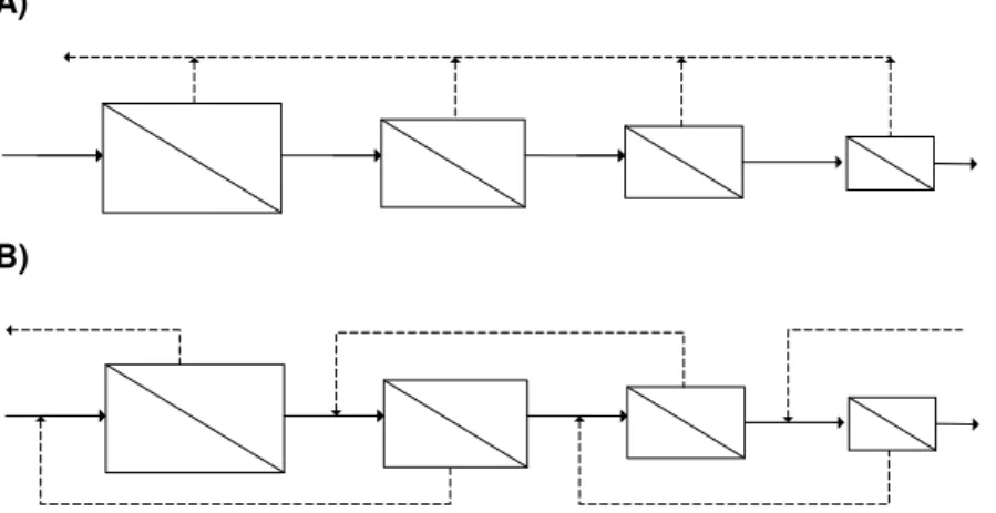
A very effective and common cascade design used is the symmetric countercurrent recycle cascade, which in some ways is very similar to a continuous distillation column (Benedict, Pigford and Levi, 1981). In the case of the countercurrent recycle cascade, the permeate of a stage feeds the next upper stage, while its retentate stream is recycled back to the immediately preceding stage (Villani and Becker, 1979).

A)

P-100 _P-92

B)

P-83

Figure 1.9 – Modes of cascade operation: A) simple symmetric cascade; B) symmetric countercurrent recycle cascade (Adapted from Siew et al., 2013).

The ideal cascade proposed by Hwang, assumes that the compositions of permeate and retentate streams that make up the feed to interior stages are kept constant, which means that there is no mixing of streams of different compositions between stages, and so there are no losses of separative work. To meet the no-mix criteria the flow rate between stages and the size of each stage must vary, which means that each stage has to be of different size. In addition, the feed is introduced within the cascade where the retentate composition is the same as the feed ( Hwang and Kammermeyer, 1965).

In spite of the fact that ideal cascades minimize the energy consumptions and the global size of the plant, its assembling is complicated in terms of design, fabrication, operation and maintenance (McCandless, 1990; McCandless and Herbst, 1990). The solution to this problem in practical terms of cascade design is to approximate the ideal cascade by a small number of squared cascade segments connected in series, in what is called a squared-off cascade. With this configuration, all of the stages can be made identical and so a large reduction in the cost of separative units can be achieved (McCandless and Herbst, 1990).

(41)

1.2.3.2 Membrane cascade applications

After the huge advance in membrane cascade theory during the 1940s (Mulder, 1996; Hwang and Kammermeyer, 1975; Halle and Shacter, 2000), a lot of authors started proposing different cascade schemes, derived from the countercurrent recycle cascade, for the separation of binary systems (McCandless and Herbst, 1990; Agrawal and Xu, 1996; Yan and Kao, 1989; McCandless, 1985; Keureties et al., 1992).

Cascade design has been widely used not only for gas separation but also for liquid separation (McCandless, 1985) and solid fractionation (Vanneste et al., 2011)

Most of the studies on membrane cascades for the purification of liquid solutions are related to wastewater treatment. Several authors like Evangelista (1987) and Maskan et al. (2000) developed design methodologies to optimize RO network configurations and operating conditions.

Peng and Tremblay (2008) designed and tested a pilot scale membrane cascade system using MF, UF and NF membranes to remove oil and grease from bilge water accumulated in ships. The authors concluded that it is possible to reduce the oil and grease content of water to the allowable discharge limit through the proper design of the membrane system, selection of appropriate membranes, determination of optimal operating parameters, and assessment membrane performance.

The increasing need for a continuous, high-throughput, economical and easily scalable separation process for downstream processing of biological substrates, like proteins, carbohydrates, plasmids, viruses, organelles, and even whole cells, led Lightfoot (2005) to propose membrane countercurrent cascades as an alternative for chromatography and simulated moving bed chromatography. He and his co-workers also proposed (2008) an extended version of the binary ideal cascade theory for modeling diafiltration membrane cascades for fractionation of binary systems of two solutes in a single solvent. Each stage of a diafiltration membrane cascade consists of a UF module combined with a RO module to remove excess solvent from the permeate stream.

(42)

(43)