The impact of quantitative methods on equity mutual funds' performance

THE IMPACT OF QUANTITATIVE METHODS ON THE

PERFORMANCE OF EQUITY MUTUAL FUNDS

David Matias Fernandes

Dissertation submitted as partial requirement for the conferral of Master in

Management

Supervisor:

Prof. Doutor António Manuel Corte Real de Freitas Miguel, ISCTE Business School,

Department of Finance

II

THE IMPACT OF QUANTITATIVE METHODS ON THE

PERFORMANCE OF EQUITY MUTUAL FUNDS

ABSTRACT

In this study, we analyze the impact of using quantitative methods in fund management on the performance of equity mutual funds using a sample of US mutual funds in the 2000-2015 period.

Our results show that quantitative funds tend to underperform when compared to non-quantitative funds. We also show that fund size decreases more the performance of non-quantitative funds, while fund family size penalizes more the performance of these funds. Regarding the effect of 2007-2008 crisis on the performance of quantitative equity mutual funds, we do not find statically significant differences between quantitative and non-quantitative funds.

JEL code: G11, G23, G41

Keywords: Mutual Funds; Mutual Fund Performance; Quantitative Methods and the impact on performance equity mutual funds’; Decision-making process

III

RESUMO

Neste estudo, analisamos o impacto da utilização de métodos quantitativos pela equipa de gestão na performance de fundos de investimento em ações usando uma amostra de fundos de investimento em dos Estados Unidos da América no período 2000-2015.

Os nossos resultados mostram que os fundos quantitativos tendem a ter um desempenho inferior comparativamente ao dos fundos não quantitativos. Também mostramos que o tamanho do fundo diminui mais o desempenho dos fundos quantitativos, enquanto o tamanho da família do fundo penaliza mais o desempenho desses fundos. Em relação ao efeito da crise de 2007-2008 na performance dos fundos de investimento em ações quantitativos, não se verificaram diferenças significativas.

Palavras-Chave: Fundos de Invesitmento; Performance de fundos de investimento; Metodos quantitativos e o seu impacto na performance de fundos de investimento; Processo de tomada de decisão.

IV

ACKNOWLEDGEMENTS

I would like to thank everyone who directly and indirectly contributed to the completion of this important stage of my life - this master thesis and the consequent acquisition of the title of master.

Firstly, I would like to thank all my family, who always supported me, encouraged and motivated. Without their support, clearly it would be impossible to achieve this objective.

Secondly, I would like to thank my supervisor Professor António Freitas Miguel for the patience, wisdom and dedication in this dissertation.

I also would like to thank all my friends that motivated and encouraged me during this dissertation.

V

INDEX OF CONTENT

1. INTRODUCTION ... 1

2. LITERATURE REVIEW ... 2

2.1 Fund size ... 2

2.2 Fund family size ... 3

2.3 Age ... 3 2.4 Expenses ... 3 2.5 Loads ... 3 2.6 Flows ... 4 2.7 Past performance ... 4 2.8 Management Structure ... 5

2.9 Quantitative approach on stock selection ... 5

2.10 Previous studies ... 6

3. DATA AND VARIABLES CONSTRUCTION ... 8

3.1 Data ... 8

3.2 Variables construction ... 9

3.2.1 Mutual fund performance ... 10

3.2.2 Fund size and fund size family ... 11

3.2.3 Fund age ... 12

3.2.4 Total expense ratio and loadings ... 12

3.2.5 Flows ... 12 3.2.6 SMB and HML Loadings ... 13 4. METHODOLOGY ... 13 5. EMPIRICAL RESULTS ... 16 6. ROBUSTNESS TESTS ... 22 7. CONCLUSIONS ... 23 REFERENCES ... 24 APPENDIXES ... 27

VI

INDEX OF TABLES

Table 1 - Evolution of equity mutual funds by year ... 9

Table 2 - Fund variables ... 11

Panel A – Non-quantitative funds ... 11

Panel B - Quantitative funds ... 11

Panel C - Pairwise correlations among these fund-characteristics ... 13

Table 3 – Mutual Fund performance and quantitative methods ... 17

Panel A – Regression of quantitative dummy and fund control variables ... 17

Panel B – Interactions between quantitative funds variable and the different fund control characteristics ... 18

Panel C - Results of SUR testing differences in performance between quantitative and non-quantitative funds during the 2007-2008 crisis ... 21

VII

MAIN ABREVIATIONS USED

CAPM - Capital Asset Pricing Model

EFAMA - European Fund and Asset Management Association

CRSP - Center for Research in Security Prices

ICI - Investment Company Institute

HML - High Book-To-Market Equity Minus Low Book-To-Market Equity

MOM - Momentum

SMB - Small Market Equity Minus Big Market Equity

SUR - Seemingly Unrelated Regression

TNA - Total Net Assets

1

1. INTRODUCTION

Mutual funds have been widely used as investment vehicle for retail and institutional investors and the proof of this evolution is the growing in total net assets and in the wide variety of funds available to investors. According to the Investment Company Institute (ICI, 2019), at the end of 2018, the total net assets of worldwide regulated open-end funds managed up to $46.7 trillion, showing that on average the TNA is growing at an annual growth rate of 4.85% (since 2009) and 118,978 regulated funds were available for sale, representing an annual growth rate of 3.67% (since 2009). Equity mutual funds represent a significant part of this universe, with $9.2 trillion and 9,599 funds available to invest in the U.S. alone. Alongside with the large market of equity mutual funds, there are many investment funds available to institutional and retail investors (who hold 89% of the total assets of equity mutual funds) and when comes to pick the equity mutual fund, investors wonder themselves: which fund and how to choose from a so big variety?

Performance is important when comes to select equity funds. Jensen (1968), Malkiel (1995) and Carhart (1997) when studying the performance of mutual funds against their benchmarks get very similar findings. They conclude that in general mutual funds do not beat their passive benchmarks, on the other hand, Ippolito (1989) finds that mutual fund risk-adjusted returns, net of fees and expenses, are comparable to index funds, while Hendricks, Patel and Zeckhauser (1993) suggest that there are mutual fund managers that have “hot hands”, meaning that they are able to outperform the benchmarks but only during a short period of time. There are factors that have impact on the performance of mutual funds, including size, family size, age, fees and expenses, loads, flows, and past performance.

In this study, we use a sample of U.S. equity funds, covering the period from 2000 to 2015, to investigate if the use of quantitative methods on the investment process, allows fund managers to generate superior returns. Despite the increasing number of mutual funds using quantitative methods in their investment selection, only a few studies have tried to explain the impact of these methods on fund performance.

The remainder of this paper is structured as follows. In the next section we present the literature review. Section 3 describes our sample and data construction. Section 4 outlines the methodology. Section 5 reports our empirical results, Section 6 presents the result of robustness tests and Section 7 concludes.

2

2. LITERATURE REVIEW

Mutual funds managers want to improve their performance and the literature has been trying to find what fund characteristics impact on the performance of mutual funds. These fund characteristics include fund size, fund family size, age, expenses, loads, flows, past performance, and management structure. It is important to note that the literature presented below concerns specifically to U.S. equity mutual fund industry and, according to Ferreira, Keswani, Miguel and Ramos (2013), these results cannot be directly extrapolated to other mutual fund industries.

2.1 Fund size

The relation between size and performance of mutual funds is probably the most studied and discussed relation in the academic field. What academics try to explain is if the size of the fund has a direct impact on its performance.

Theoretically, larger funds have advantages and disadvantages over smaller funds. The advantages that possibly exist are: larger funds can spread the fixed expenses over a larger asset base and have more resources for research; benefit from investment opportunities that are not available to smaller funds; the capacity to negotiate better spreads (because they have larger positions and larger trading volumes) (Ferreira et al., 2013) and benefit from the fact that brokerage commissions decline with the size of transactions (Brennan and Hughes, 1991).

On the other hand, there are some disadvantages too, once larger funds are not able to scale infinitely their investments which is a determinant of performance persistence (Gruber, 1996; Berk and Green, 2004). Grinblatt and Titman (1989) find that fund size has a positive impact on performance, being the smaller funds the ones with better performance, however later, the research of the same authors does not back their previous work, once the authors claim “that performance is positively related to portfolio turnover, but not to the size of the

mutual funds” (Grinblatt and Titman, 1994: 438). A large part of the literature seems to support

the theory that larger funds perform worse than smaller funds due to diseconomies of scale, pointing the big problem to the illiquidity of stocks. For example, Chen, Hong, Huang and Kuik (2004: 1) argues that “fund returns, both before and after fees and expenses, decline with

lagged fund size” and this is more “pronounced among funds that have to invest in small and illiquid stocks, suggesting that these adverse scale effects are related to liquidity”. They also

3 liquidity constraints hypothesis (Chen et al., 2004). Later, Pollet and Wilson (2008) back Chen

et al., (2004) studies, concluding that managers tend to keep investing on a “few best bets”

(stocks) when the fund receives inflows instead of diversifying into other assets, and this leads to the liquidity constraints hypothesis.

2.2 Fund family size

Some mutual funds belong to a “family”, this means that some funds are “developed” under the same investment company. Here, contrary to what happens on “fund size” economies of scale and scope at fund family level can exist, being the arguments that certain expenses like research and administrative can be shared among funds (Ferreira et al., 2013). Chen et al., (2004), Agnesens (2013) and Ferreira et al., (2013) find that fund family size has a positive and statistically significant effect on performance and according to Chen et al., (2004) this advantage comes from the economies of scale from trading commissions and lending fees.

2.3 Age

When new funds are created, they are subject to very high upfront costs and have less experience on the market than older funds and this can have an impact on their performance (Ferreira et al., 2013), however, Chen et al., (2004) and Ferreira et al., (2013) find no evidence that there is a relationship between performance and age.

2.4 Expenses

Mutual fund expenses (including management fees) are the price that investors pay for professional managers to invest their money, however it seems that investors pay little attention to this factor in the mutual fund selection process (Capon, Fitzsimons, and Prince, 1996).

The impact of expenses on equity mutual fund performance has been largely studied. Carhart (1997), Pollet and Wilson (2008) and Gil-Bazo and Ruiz Verdu (2009) find a negative relation of expenses with net-fee performance, while Chen et al., (2004) and Ferreira et al., (2013) do not find any relation between fees and performance.

2.5 Loads

Loads are “fees” that investors must pay to enter (front-end load) or to exit (back-end load/redemption fee) the mutual fund. The objective of a back-end load is to discourage investors from exiting the fund, what is likely to happen when funds underperform.

4 Consequently, this “fee” allows mutual fund managers freedom to take risks and have abnormal returns (Chordia, 1996).

Chen et al., (2004) and Ferreira et al., (2013) states that there is no statistically significant relation between performance and loads, on the other hand, Carhart (1997) and Pollet and Wilson (2008) find an inverse relationship between performance and loads.

2.6 Flows

Mutual fund flows are presented as the difference between inflows and outflows during a specific period, meaning that this metric shows whether investors are putting their money into a mutual fund or taking it from the mutual fund. Gruber (1996) and Zheng (1999) find evidence that mutual funds that have inflows have better performance than mutual funds that have outflows, however in their studies, the model they use to measure performance does not consider the momentum factor. The momentum factor is considered in the Carhart four-factor model (Carhart, 1997) to measure performance and incorporates the tendency for, for example, a stock price to continue rising if it is going up or continue declining if it is going down and this can be driven by supply and demand which is related to inflows/outflows on mutual funds. Sapp and Tiwari (2004) and Ferreira et al., (2013) use the Carhart four-factor model in their studies and do not find any significant relation between performance and flows.

2.7 Past performance

Capon, Fitzsimons, and Price (1996) find that when investors search for a mutual fund to invest, the metric that they attribute most importance to is the “investment performance track record”, in other words past performance. This is true even, knowing that past performance does not necessarily mean future performance. This theory is compatible with the studies of Patel, Zeckhauser, and Hendricks (1993) that report that previous fund performance (adjusted for risk) is associated with new inflows to mutual funds.

Malkiel (1995), Carhart (1997), Ferreira et al., (2018) on their studies, concluded that there is not long-term persistence on performance, meaning this that, the fact that the fund has achieved a positive return in the past, does not mean that this will happen in the future. However, there are some authors, including Hendricks, Patel, & Zeckhauser (1993) that claim that there are mutual fund managers that have “hot hands”, meaning that they are able to outperform the benchmarks during a short period of time.

5

2.8 Management Structure

The management structure referees basically to who makes the decisions on and choose how they are taken. This management structure can vary from a solo manager to a large team of managers, where the decision-making power can be centralized on a few or all managers. Han, Noe and Rebello (2012) study how management structure has impact on the mutual fund performance and came to some interesting conclusions. According to their studies, team-managed funds perform better, allocate their funds more conservatively, and trade less aggressively than single manager funds, besides that, these mutual funds deviate less from benchmarks and trade with less respect to new information than single managed funds.

However, the conclusions on this topic are not consensual and other authors did not come to the same conclusions. For example, Bliss, Potter and Schwarz (2008) show that there is no significant difference between mutual funds that are team-managed and single-managed, while Chen et al., (2004), Massa, Reuter and Zitzewitz (2010) and Ferreira et al., (2013) find that team-managed funds perform worse than single-managed.

2.9 Quantitative approach on stock selection

The quantitative classification is attributed when the decision to buy or sell assets is mostly made by a previously defined mathematical model and non-quantitative1 when the decision is made mostly from human judgment.

The use of quantitative methods in the area of financial markets is not exactly new. It has been used, at least, since the development of the Modern Portfolio Theory (Markowitz, 1952). The model was developed for risk management, however, as Fabozzi, Focardi and Jonas (2007) indicate in their survey about the challenges in quantitative equity management, now quantitative methods are being used to find positive alphas instead of being used solely and exclusively to risk management. According to Yale Insights (2019) quantitative methods in recent years have been evolving in financial markets due to improvements in machine learning and artificial intelligence.

Funds that employ quantitative methods typically tend to look for unique and specific characteristics in a large universe of stocks (due to their high processing capacity) while funds

6 that do not employ quantitative methodologies tend to do exhaustive analysis on each company (Lawson, 2000).

The expected advantages when implementing the use of quantitative methods in an investment firm are cost savings, the ability to identify and exploit short-lived market inefficiencies and remove behaviors biases from decision making process (Gregory-Allen, Shawky and Stangl, 2009). The role of behavioral biases in financial markets is already notably documented in Khaneman and Tversky (1979 and 1991), in which they show that decision makers are exposed to behavioral biases and leading to irrational decisions. One of the main goals of quantitative methods is to avoid this. As Fabozzi, Focardi and Jonas (2008: 659) state: “An analyst might fall in love with the Chief Financial Officer of a firm and lose his objectivity”.

However, not everything is perfect as these quantitative models fail to analyze what is not quantifiable, for example the quality of firm management. Moreover, these models tend to be based on past relationships that may change in the future (Ahmed and Nanda, 2005).

The question arises: do quantitative funds really perform better?

2.10 Previous studies

The literature on the different characteristics between quantitative and non-quantitative funds is not extensive, however, some authors have already studied the subject using different approaches, covering different time periods and using different databases and did not come to a consensus regarding performance. In this subsection we provide an overview of the research already done.

On the one hand, Wermers, Yao and Zhao (2007), Gregory-Allen et al., (2009) and Abis (2017) find evidence that quantitative equity funds have worse performance than non-quantitative. Wermers et al., (2007), using a CSRP Survivor-bias free mutual fund database covering the period from 1980 to 2002, forecasts stock returns using known anomalies2 claiming that anomalies are usually exploited by quantitative funds and concludes that they do not produce abnormal returns and deduces that the abnormal returns obtained by mutual funds must have been produced by non-quantitative information. Later, Gregory-Allen et al., (2009), analyzing the period from 2002 to 2006, using a PSN Database and a questionnaire where mutual funds were divided into groups according to their primary investment process, supports Wermers’ et al., (2007) findings, concluding that fundamental analysis (comparing with

7 bottom-up, top-down, quantitative, computer screening and technical analysis approaches) have significantly better performance3_{. Abis (2017) analyze the period from 1999 to 2015 with}

a CSRP Mutual Fund dataset and find evidence that quantitative mutual funds have worse performance than non-quantitative.

On the other hand, Ahmed and Nanda (2005) and Zhao (2006) find different results. Ahmed and Nanda (2005), analyze a small set of enhanced index equity funds4 from Morningstar on Disc database5. The authors classify these funds as quantitative or fundamental and into large cap growth, large-cap value, small cap growth or small cap value and concluded that enhanced index funds that use quantitative methods beat their benchmarks and that only quantitative funds that invest in small cap growth stocks achieve positive alphas. Zhao (2006), using CSRP Mutual Fund Database from 1994 to 2003 find that quantitative and non-quantitative funds have similar performance even though non-quantitative funds have lower risk.

Regarding the behavior of equity mutual funds specifically during crises, Zhao (2006) and Abis (2017) also came across different conclusions. Zhao (2006) claims that quantitative funds have better performance during crises while Abis (2017) who studied the period that cover the subprime crisis has a different conclusion: during market downturns non-quantitative funds have better performance than quantitative ones, probably due to the lack of flexibility that quantitative funds have. Several other authors have discussed the impact of quantitative methods on previous crises in the context of hedge funds, for example, Khandani and Lo (2007) and Fabozzi et al., (2008: 659) claim that quantitative funds use correlated strategies (supporting the lack of flexibility evidenced by Abis (2017)), what leads to liquidity problems when they need to “unwind” their portfolios. About performance in non-crises periods and analyzing two expansion periods Abis (2017: 5) concludes that “the performance of

quantitative funds in expansions has been declining over time due to “overcrowding”, caused by the increase in the share of quantitative funds in the market and their tendency to hold overlapping portfolios”.

Concerning stock holdings, Zhao (2006) and Abis (2017) come to similar findings: due to a big capacity to process information, quantitative funds can cover a bigger range of stocks and consequently hold more stock what leads to a better portfolio diversification and lower idiosyncratic volatility. Zhao (2006) notes that quantitative funds have few managers and

3_{The author acknowledges that the time period the sample is not representative for different market trends.} 4_{Fund that uses active management to modify the weights of holdings for additional return.}

8 higher costs when it comes to trading costs due to superior activity with illiquid stocks. Abis (2017) claims that quantitative funds tend to invest in stocks with a “longer story” and superior media and analyst coverage and that these stocks have worse performance than younger and less covered stocks (that are more picked by quantitative funds). She also finds that non-quantitative funds have their holdings more disperse than non-quantitative (even though they have less stocks on their holdings).

As regarding fund size, Zhao (2006) and Abis (2017) find that quantitative funds are smaller and Zhao (2006) analyzing the relation fund size-performance through a Fama-MacBeh regression finds that the adverse size effect is more pronounced among quantitative funds6_.

In what concerns expenses Zhao (2006) and Abis (2017) are unanimous: quantitative funds have lower expense ratios, supporting the theory that quantitative funds have lower operating costs.

3. DATA AND VARIABLES CONSTRUCTION

3.1 Data

The sample used in this study is provided by Lipper Hindsight database and contains data for the period 2000-2015. The data is survivorship bias free (i.e., includes active and defunct funds), with quarterly data observations. We should note that the period covers diverse market trends (crisis7 and non-crisis periods), transforming this sample temporally representative.

At the end of 2015, our sample represents $8.525 trillions of Total Net Assets, while according to EFAMA, in the USA were managed $9.943 trillion, meaning this that our sample covers around 86% of the TNA covered by EFAMA. Analyzing the number of funds covered, we find that our sample includes 3,368 equity mutual funds, while EFAMA counts 6,162 meaning that our sample covers 55% of the equity mutual funds.

We established different filters to define our final sample. We only work with actively managed equity mutual funds and domiciled in U.S. (we only have a quantitative classification for U.S. funds) and exclude funds of funds, close end, enhanced index and index tracking funds, in order to assess the “freely” management skill of fund more accurately. In addition, we only include in our sample funds that have at least 36 continuous monthly observations, to ensure

6_{Supporting Berk and Green (2004) theory about fund size and performance.}

9 that we have enough observations to compute significant lagged returns and risk-adjusted returns measures. Moreover, to prevent double counting funds, we follow the approach of Ferreira et al., (2013) and Demirci, Ferreira, Matos and Siam (2019) and use only primary share classes in our sample, excluding multiple share classes of the same fund.

The classification of mutual funds as quantitative or non-quantitative is also provided by Lipper Hindsight database and results from information provided by mutual fund prospectus, being defined as quantitative a mutual fund that “uses rule-based mathematical

models in order to initiate buy and sell decisions”8. The mutual funds that do not fit this description are considered non-quantitative.

Table 1 presents number and TNA funds by year for quantitative and non-quantitative funds in our sample and shows that non-quantitative funds have a dominant share of the industry and in what concerns TNA they tend to dominate and increase their share over the years. However, when we look at the number of funds that employ quantitative methods, we observe an increasing number of funds and an increasing bigger share of the market.

Table 1 - Evolution of equity mutual funds by year

This table presents the number of funds and TNA of quantitative and non-quantitative funds by year Data is from Lipper Hindsight database. See Appendix I for variables definition.

Quantitative funds Non-quantitative funds Total Year TNA ($M) TNA (% of all) Number Number (% of all) TNA ($M) TNA (% of all) Number Number (% of all) TNA ($M) Number 2000 91,631 3.43% 72 3.64% 2,579,117 96.57% 1,906 96.36% 2,670,748 1,978 2001 78,504 3.31% 85 3.72% 2,289,910 96.69% 2,200 96.28% 2,368,414 2,285 2002 56,582 3.01% 89 3.68% 1,823,383 96.99% 2,328 96.32% 1,879,965 2,417 2003 77,749 2.97% 99 3.96% 2,541,152 97.03% 2,403 96.04% 2,618,901 2,502 2004 92,617 2.96% 109 4.20% 3,034,336 97.04% 2,484 95.80% 3,126,953 2,593 2005 100,940 2.85% 113 4.34% 3,435,868 97.15% 2,491 95.66% 3,536,808 2,604 2006 121,323 2.89% 125 4.79% 4,070,445 97.11% 2,484 95.21% 4,191,768 2,609 2007 124,829 2.70% 135 5.24% 4,503,231 97.30% 2,442 94.76% 4,628,060 2,577 2008 67,726 2.62% 137 5.33% 2,518,474 97.38% 2,433 94.67% 2,586,200 2,570 2009 85,682 2.49% 161 6.19% 3,358,842 97.51% 2,441 93.81% 3,444,524 2,602 2010 92,412 2.33% 180 6.85% 3,872,461 97.67% 2,448 93.15% 3,964,873 2,628 2011 86,212 2.40% 199 7.55% 3,513,345 97.60% 2,437 92.45% 3,599,557 2,636 2012 92,100 2.29% 198 7.53% 3,936,982 97.71% 2,432 92.47% 4,029,082 2,630 2013 123,160 2.33% 199 7.58% 5,151,505 97.67% 2,426 92.42% 5,274,665 2,625 2014 136,445 2.47% 198 7.65% 5,385,858 97.53% 2,391 92.35% 5,522,303 2,589 2015 139,900 2.66% 192 7.65% 5,113,774 97.34% 2319 92.35% 5,253,674 2,511

3.2 Variables construction

In this section, we describe the variables used in our regressions and explain their presence in our sample. The dependent variable is mutual fund performance, while the

10 level control variables include size, family size, age, total expense ratio, loads, flows, past performance, HML and SMB.

3.2.1 Mutual fund performance

We measure performance of mutual funds using four-factor alpha (Carhart, 1997). The four-factor alpha model (Carhart, 1997) incorporates the CAPM model (Sharpe, 1964), two factors from the three-factor alpha model (Fama and French, 1992) – SMB (Small Market Equity minus Big Market Equity) and HML (High B/M Equity and Low B/M Equity) and an

anomaly found by Jogadeesh and Titman (1993) – Momentum.9

The model is explained by the following equation:

𝛼𝑖 = 𝑅𝑖𝑡− (𝛽0𝑖𝑅𝑀𝑡+ 𝛽1𝑡𝑆𝑀𝐵𝑡+ 𝛽2𝑡𝐻𝑀𝐿𝑡+ 𝛽3𝑡𝑀𝑂𝑀𝑡+ 𝜀)

𝛼_𝑖: is the excess of return according to benchmark index and risk-free adjusted with four factors;

𝛽_𝑖: are the loadings on each factor;

𝑅𝑖𝑡: is the realized return of fund i in quarter t;

𝑅𝑀_𝑡: is the expected return by investors according to the risk of fund at the end of the quarter

t;

𝑆𝑀𝐵_𝑡: is the difference between the average return of the three smaller and bigger portfolios according to their market equity at the end of year t;

𝐻𝑀𝐿𝑡: is the difference between the average return of two portfolios with the highest and

lowest ration B/M at the end of year t;

𝑀𝑂𝑀_𝑡: is the difference between the portfolio with the highest return in the past 12 months and the portfolio with the lowest return in the past 12 months of year t;

𝜀 : is a generic error that is not correlated with any of the independent variables.

In order to remove extreme values from our sample we winsorized the sample, removing 1% of the values from the top and bottom of the distribution.

9

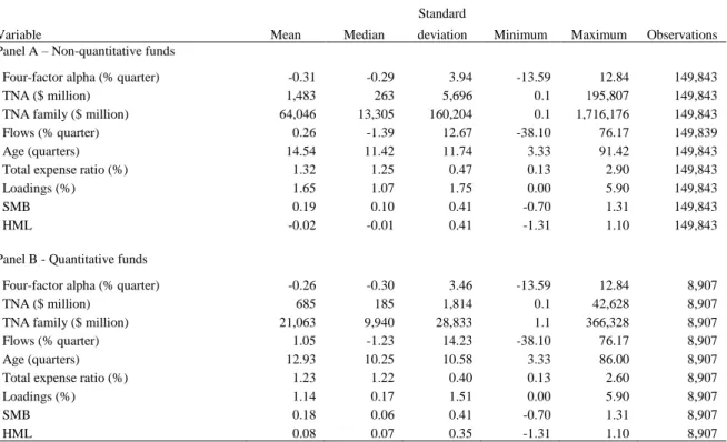
11 From Table 2 we can see that quantitative and non-quantitative funds have, on average, negative returns, however we should note that non-quantitative funds have worse results than qualitative funds (-0.31% versus -0.26%).

Table 2 - Fund variables

Panel A and Panel B present fund level variables averaged across fund quarters for the period 2000–2015, for non-quantitative funds and non-quantitative funds, respectively. Panel C presents pairwise correlations among these variables. Performance measure is four-factor alpha. Control variables include: fund size and fund family size, measured by fund’s TNA in millions of US dollars; fund flows in percentage (Flows); fund age in years at the end of each quarter (Age); Total expense ratio; Loads (Front-end and back-end loads); loadings on the small minus big size factor (SMB); and loadings on the high minus low book-to-market factor (HML). See Appendix I for variables definition.

Standard

Variable Mean Median deviation Minimum Maximum Observations Panel A – Non-quantitative funds

Four-factor alpha (% quarter) -0.31 -0.29 3.94 -13.59 12.84 149,843 TNA ($ million) 1,483 263 5,696 0.1 195,807 149,843 TNA family ($ million) 64,046 13,305 160,204 0.1 1,716,176 149,843 Flows (% quarter) 0.26 -1.39 12.67 -38.10 76.17 149,839 Age (quarters) 14.54 11.42 11.74 3.33 91.42 149,843 Total expense ratio (%) 1.32 1.25 0.47 0.13 2.90 149,843 Loadings (%) 1.65 1.07 1.75 0.00 5.90 149,843

SMB 0.19 0.10 0.41 -0.70 1.31 149,843

HML -0.02 -0.01 0.41 -1.31 1.10 149,843

Panel B - Quantitative funds

Four-factor alpha (% quarter) -0.26 -0.30 3.46 -13.59 12.84 8,907 TNA ($ million) 685 185 1,814 0.1 42,628 8,907 TNA family ($ million) 21,063 9,940 28,833 1.1 366,328 8,907 Flows (% quarter) 1.05 -1.23 14.23 -38.10 76.17 8,907 Age (quarters) 12.93 10.25 10.58 3.33 86.00 8,907 Total expense ratio (%) 1.23 1.22 0.40 0.13 2.60 8,907

Loadings (%) 1.14 0.17 1.51 0.00 5.90 8,907

SMB 0.18 0.06 0.41 -0.70 1.31 8,907

HML 0.08 0.07 0.35 -1.31 1.10 8,907

3.2.2 Fund size and fund size family

Fund size (TNA) is measured in millions of U.S. dollars and represents the sum of all share classes of a specific fund. From Table 2, we can see that non-quantitative funds have, on average, over two times more money under management ($1,483 million of dollars), than quantitative funds ($685 million of dollars). Regarding fund size family represents the sum of all funds TNA under the same family (and the respective share classes). Here, we observe the same tendency, non-quantitative funds, on average, belong to families three times bigger than quantitative funds ($64,046 and $21,063 million of dollars, respectively).

12

3.2.3 Fund age

In our date base, fund age is represented by the difference between the date of observation and the fund inception, measured in years. Table 2 shows that quantitative funds have smaller track record than non-quantitative (on average, 12.93 years versus 14.54 years).

3.2.4 Total expense ratio and loadings

The total expense ratio represents the percentage of total expenses annualized based on TNA (including all share classes) and the loadings represent the sum of front-end and back-end loads of mutual funds.10 From Table 2, we can see that the total expense ratio of non-quantitative funds is higher which confirms the fact that the non-quantitative funds have lower costs probably due to automation and capacity to process and interpret massive amounts of data quickly and at reduced costs by using machines, while non-quantitative funds have to rely on humans, what increases the time for processing and costs (1.32% versus 1.23%).

Concerns loadings, the average loadings of quantitative funds are lower than non-quantitative (1.65% versus 1.14%), meaning that non-non-quantitative funds are more costly to buy or sell, on average.

3.2.5 Flows

We follow the approach of Sirri and Tufano (1998) and Ferreira et al. (2013) in order to calculate fund flows. Fund flow represent the percentage of growth in total assets under management (TNA) of a mutual fund, during a period, discounting the reinvestment of dividends and distributions. In order to calculate the fund flow for fund i at quarter t, we use the following formula:

𝐹𝑙𝑜𝑤_𝑖,𝑡 = 𝑇𝑁𝐴𝑖,𝑡 − 𝑇𝑁𝐴𝑖,𝑡−1∗ (1 + 𝑅𝑖,𝑡)

𝑇𝑁𝐴_{𝑖,𝑡−1} (1)

Where:

𝑇𝑁𝐴_𝑖,𝑡 : is the total net asset value of fund i, at the end of quarter t;

𝑇𝑁𝐴_{𝑖,𝑡−1} : is the total net asset value of a fund i, at the beginning of quarter t;

13 𝑅_𝑖,𝑡 : is the raw return of fund i, at the end of quarter t.

We find in Table 2 that quantitative funds have greater flows than non-quantitative funds (1.05% versus 0.26%, respectively), meaning that quantitative funds have an inferior TNA but are growing at a faster rate than non-quantitative funds.11

3.2.6 SMB and HML Loadings

We measure fund style using the loadings on SMB and HML. From Table 2 we verify that there are no significant differences for SMB between for quantitative and non-quantitative funds. Although SMB for non-quantitative funds is slightly higher than for quantitative funds (0.19 versus 0.18), both samples have the same standard deviation. Regarding HML the two groups are different: nonquantitative funds present a lower HML than quantitative funds, -0.02 and 0.08, respectively, and non-quantitative funds have a higher standard deviation12.

When we analyze the correlation between the control variables in our study, in Table 2 – Panel C, we find that the existent correlations are comparable with that in the mutual fund literature. Since the correlation coefficients are low, multicollinearity among these variables is week, suggesting that these variables can be included together in our regressions.

Panel C - Pairwise correlations among these fund-characteristics 1 2 3 4 5 6 7 8 Size 1 1 Family size 2 0.5741 1 Flows 3 0.0201 0.0125 1 Age 4 0.3862 0.1739 -0.136 1 Expense ratio 5 -0.413 -0.306 -0.009 -0.191 1 Loads 6 0.0071 0.0708 -0.013 0.0967 0.3876 1 SMB 7 -0.115 -0.071 0.0025 -0.091 0.1631 0.0025 1 HML 8 -0.006 -0.039 0.0548 -0.037 -0.081 -0.037 -0.101 1

4. METHODOLOGY

We start by running a regression in order to determine if there are differences in mutual fund performance for those funds that use quantitative methods in their investment process. More specifically, we run panel data regression, where we regress quarterly fund performance measured by four-factor alpha on a dummy variable that is equal to one if the fund is a

11 _{Fund flows are winsorized at the bottom and top 1% level of the distribution.}

14 quantitative fund and zero otherwise. We also include in our regression all the mutual funds characteristics previously described, in order to control for differences between funds: fund size, fund family size, age, total expense ratio, loads, flows, past performance, HML and SMB. Our regression includes time and fund type fixed effects and the standard errors are clustered by fund. We therefore run the regression described in the following equation:

𝑃𝑒𝑟𝑓𝑜𝑟𝑚𝑎𝑛𝑐𝑒_𝑖,𝑡 = 𝛽₀+ 𝛽₁∗ 𝐷𝑢𝑚𝑚𝑦 𝑞𝑢𝑎𝑛𝑡𝑖𝑡𝑎𝑡𝑖𝑣𝑒_{𝑖,𝑡−1}

+𝛽₂∗ 𝐹𝑢𝑛𝑑 𝑐𝑜𝑛𝑡𝑟𝑜𝑙 𝑣𝑎𝑟𝑖𝑎𝑏𝑙𝑒_{𝑖,𝑡−1}+ 𝜀 (2)

Where:

𝐷𝑢𝑚𝑚𝑦 𝑞𝑢𝑎𝑛𝑡𝑖𝑡𝑎𝑡𝑖𝑣𝑒: the fund is quantitative;

𝐹𝑢𝑛𝑑 𝑐𝑜𝑛𝑡𝑟𝑜𝑙 𝑣𝑎𝑟𝑖𝑎𝑏𝑙𝑒𝑠 (𝑙𝑎𝑔𝑔𝑒𝑑 𝑏𝑦 𝑜𝑛𝑒 𝑞𝑢𝑎𝑟𝑡𝑒𝑟): are size, family size, age, total expense ratio, loads, flows, past performance, HML and SMB;

𝑡: is quarter t; 𝑖: is fund i;

𝜀: is generic error term that is not correlated with any of the independent variables

We also test the impact of mutual funds characteristics (size, family size, age, total expense ratio, loads, flows and past performance) on the performance of funds that use quantitative methods. In order to do that, we first generate a dummy variable for each fund control variable which we assign the value of one if the fund control variable is above-median and zero if it is below median. We then interact this dummy variable with the quantitative fund dummy. Each fund control variable is controlled on his own regression individually. In these regressions, as in the previous one, we include time and fund type fixed effects and the standard errors are clustered by fund. This regression is represented by the following equation:

𝑃𝑒𝑟𝑓𝑜𝑟𝑚𝑎𝑛𝑐𝑒_𝑖,𝑡 = 𝛽₀+ 𝛽₁∗ 𝐷𝑢𝑚𝑚𝑦 𝑞𝑢𝑎𝑛𝑡𝑖𝑡𝑎𝑡𝑖𝑣𝑒_{𝑖,𝑡−1}+ 𝛽₂ ∗ 𝐹𝑢𝑛𝑑 𝑐𝑜𝑛𝑡𝑟𝑜𝑙 𝑣𝑎𝑟𝑖𝑎𝑏𝑙𝑒_{𝑖,𝑡−1}+ 𝛽₃∗ 𝐷𝑢𝑚𝑚𝑦 𝑞𝑢𝑎𝑛𝑡𝑖𝑡𝑎𝑡𝑖𝑣𝑒_{𝑖,𝑡−1} ∗ 𝐷𝑢𝑚𝑚𝑦 𝑓𝑢𝑛𝑑 𝑐𝑜𝑛𝑡𝑟𝑜𝑙 𝑣𝑎𝑟𝑖𝑎𝑏𝑙𝑒_{𝑖,𝑡−1}+ 𝜀 (3) Where:

15 𝐹𝑢𝑛𝑑 𝑐𝑜𝑛𝑡𝑟𝑜𝑙 𝑣𝑎𝑟𝑖𝑎𝑏𝑙𝑒 (𝑙𝑎𝑔𝑔𝑒𝑑 𝑏𝑦 𝑜𝑛𝑒 𝑞𝑢𝑎𝑟𝑡𝑒𝑟): are size, family size, age, total expense ratio, loads, flows, past performance, HML and SMB;

𝐷𝑢𝑚𝑚𝑦 𝑓𝑢𝑛𝑑 𝑐𝑜𝑛𝑡𝑟𝑜𝑙 𝑣𝑎𝑟𝑖𝑎𝑏𝑙𝑒: the fund control variable value is above-median (lagged by one quarter);

𝑡: is quarter t; 𝑖: is fund i;

𝜀: is generic error term that is not correlated with any of the independent variables

Finally, we test the impact of the usage of quantitative methods on mutual fund performance during crisis periods using seemingly unrelated regressions (SUR). We split our sample in two subsamples: one with observations that belong to quantitative funds and another one with observations that belong to non-quantitative funds. We then regress performance on a dummy variable that is equal to one in the 2007-2008 period and zero otherwise. As before, we use control variables, include time and fund type fixed effects and the standard errors are clustered by fund. The regression is represented by the following equation:

𝑃𝑒𝑟𝑓𝑜𝑟𝑚𝑎𝑛𝑐𝑒_𝑖,𝑡

= 𝛽₀+ 𝛽₁∗ 𝐷𝑢𝑚𝑚𝑦 𝑐𝑟𝑖𝑠𝑖𝑠_{𝑖,𝑡−1}+ 𝛽₂∗ 𝐹𝑢𝑛𝑑 𝑐𝑜𝑛𝑡𝑟𝑜𝑙 𝑣𝑎𝑟𝑖𝑎𝑏𝑙𝑒_{𝑖,𝑡−1} + 𝜀

(4)

Where:

𝐷𝑢𝑚𝑚𝑦 𝑐𝑟𝑖𝑠𝑖𝑠: the observation belongs to a crisis period (from third quarter of 2007 to end of 2008);

𝐹𝑢𝑛𝑑 𝑐𝑜𝑛𝑡𝑟𝑜𝑙 𝑣𝑎𝑟𝑖𝑎𝑏𝑙𝑒𝑠 (𝑙𝑎𝑔𝑔𝑒𝑑 𝑏𝑦 𝑜𝑛𝑒 𝑞𝑢𝑎𝑟𝑡𝑒𝑟): are size, family size, age, total expense ratio, loads, flows, past performance;

𝑡: is quarter t; 𝑖: is fund i;

16

5. EMPIRICAL RESULTS

In this section we present the results of the regressions presented in the previous section. Firstly, we present the regression results which are intended to determine if there are differences in the performance of quantitative and non-quantitative equity mutual funds (in Panel A, Table 3), then we present the different regressions where we test the impact of the different fund characteristics on the performance of quantitative funds (Panel B, Table 3), and finally we present the results of the seemingly unrelated regressions (SUR) which aims to identify whether there are changes in the performance of quantitative and non-quantitative funds during periods of crisis (Panel C, Table 3).

17 Table 3 – Mutual Fund performance and quantitative methods

This table presents the regression results of regressing quarterly performance measured using four-factor alpha. Panel A reports the results from equation (2) where we regress the quantitative funds variable with control fund characteristics. In Panel B we present the interactions between quantitative funds variable and the different fund control characteristics to understand the impact of the fund characteristics in quantitative funds’ performance. In Panel C we present the results of the seemingly unrelated regressions where we test the difference of performance between quantitative funds during crisis. * is used to indicate the level of significance at 10%, ** 5% and *** 1%. See Appendix I for further details about variables.

Panel A – Regression of quantitative dummy and fund control variables using 4-factor alpha

(1)

Quantitative -0.0007**

(-2.03)

Size (log) -0.0007***

(-8.27) Family size (log) 0.0005***

(9.04)

Age (log) 0.0002

(0.97) Total Expense Ratio -0.2083***

(-5.76) Loads -0.0151** (-1.97) Flow -0.0009 (-1.04) Past Performance 0.0598*** (15.16) SMB -0.0002 (-0.61) HML 0.0051*** (15.00) Time fixed effects Yes Fund type fixed effects Yes Number of observations 158,750 Adjsted R-squared 0.065

Analyzing column (1) of Panel A (Table 3), we find statistically significant results that indicate that quantitative funds perform worse than non-quantitative funds. On average, quantitative funds outperform non-quantitative funds by 7 basis points per quarter. This result is consistent with the findings in Wermers et al., (2007), Gregory-Allen et al., (2009) and Abis (2017). Regarding the coefficients on fund characteristics for U.S., in general, our results are consistent with the findings in the literature.

18 Panel B – Interactions between quantitative funds variable and the different fund control characteristics using 4-factor alpha

(1) (2) (3) (3) (4) (5) (6) (7) (8)

Quantitative 0.0001 -0.0000 -0.0004 -0.0012** -0.0011** 0.0000 -0.0005 -0.0017*** -0.0008 (0.23) (-0.01) (-0.82) (-2.37) (-2.30) (0.01) (-1.04) (-3.40) (-1.44) Size (log) -0.0006*** -0.0007*** -0.0007*** -0.0007*** -0.0007*** -0.0006*** -0.0007*** -0.0006*** -0.0007***

(-7.90) (-8.31) (-8.26) (-8.26) (-8.28) (-8.25) (-8.27) (-8.26) (-8.27) Size (log) x Quantitative -0.0020***

(-2.69)

Family size (log) 0.0005*** 0.0006*** 0.0005*** 0.0005*** 0.0005*** 0.0005*** 0.0005*** 0.0005*** 0.0005***

(9.00) (9.09) (9.02) (9.05) (9.05) (9.03) (9.04) (9.07) (9.04)

Family size (log) x Quantitative -0.0016** (-2.20)

Age (log) 0.0002 0.0002 0.0002 0.0002 0.0002 0.0002 0.0002 0.0002 0.0002

(0.99) (0.96) (1.08) (0.97) (1.00) (0.95) (0.97) (0.94) (0.98)

Age (log) x Quantitative -0.0008

(-0.98)

Total Expense Ratio -0.2091*** -0.2084*** -0.2083*** -0.2125*** -0.2081*** -0.2086*** -0.2083*** -0.2077*** -0.2083*** (-5.79) (-5.77) (-5.76) (-5.78) (-5.76) (-5.77) (-5.76) (-5.75) (-5.76)

Total Expense Ratio x Quantitative 0.0010

(1.22) Loads -0.0149* -0.0148* -0.0152** -0.0151** -0.0163** -0.0152** -0.0151** -0.0150* -0.0152** (-1.95) (-1.93) (-1.99) (-1.97) (-2.08) (-1.98) (-1.97) (-1.96) (-1.98) Loads x Quantitative 0.0009 (1.39) Flow -0.0009 -0.0009 -0.0009 -0.0009 -0.0009 -0.0007 -0.0009 -0.0009 -0.0009 (-1.03) (-1.04) (-1.04) (-1.05) (-1.04) (-0.80) (-1.04) (-1.05) (-1.04) Flow x Quantitative -0.0015*

19 (-1.85)

Past Performance 0.0598*** 0.0598*** 0.0598*** 0.0598*** 0.0598*** 0.0598*** 0.0600*** 0.0598*** 0.0598*** (15.14) (15.15) (15.15) (15.15) (15.16) (15.15) (15.02) (15.15) (15.16)

Past Performance x Quantitative -0.0004

(-0.55) SMB -0.0002 -0.0002 -0.0002 -0.0002 -0.0002 -0.0002 -0.0002 -0.0003 -0.0002 (-0.61) (-0.65) (-0.60) (-0.59) (-0.61) (-0.60) (-0.61) (-0.97) (-0.61) SMB x Quantitative 0.0020** (2.58) HML 0.0051*** 0.0051*** 0.0051*** 0.0051*** 0.0051*** 0.0051*** 0.0051*** 0.0051*** 0.0051*** (15.00) (14.99) (15.00) (14.98) (14.97) (15.00) (15.00) (14.96) (14.74) HML x Quantitative 0.0001 (0.17)

Time fixed effects Yes Yes Yes Yes Yes Yes Yes Yes Yes

Fund type fixed effects Yes Yes Yes Yes Yes Yes Yes Yes Yes

Number of observations 158,750 158,750 158,750 158,750 158,750 158,750 158,750 158,750 158,750

20 Fund size has a negative effect on performance which is in line with findings in e.g., Grinblatt and Titman (1989) and Chen et al. (2004). Concerning family size our results indicate that the performance of mutual funds improves when the fund belongs to larger families, which is consistent with findings in Chen et al. (2004), Agnesens (2013), and Ferreira et al., (2013). Regarding total expense ratio and loads we find that higher expenses and loads erode fund performance which is consistent with Carhart (1997). We also find that funds that performed better in the past tend to perform better in the future, which contrasts with the findings in Malkiel (1995), Carhart (1997), Ferreira et al., (2018).

Concerning the impact of funds characteristics on the performance of mutual funds that apply quantitative methods in their investment process, in Table 3, Panel B, we find that fund size has a negative impact in the performance of quantitative funds when comparing with non-quantitative funds. This finding supports the results in Zhao (2006). There are several hypotheses that possibly could explain this phenomenon. One of the arguments supporting economies of scale for mutual funds is that larger funds have a larger asset base to spread fixed expenses (Ferreira et al., 2013), however, considering that quantitative funds have lower expenses compared to non-quantitative, proportionally the impact of this factor should become less relevant to the performance of these funds when comparing with non-quantitative funds. Another aspect that may influence this relation is that larger funds generally benefit from lower brokerage and trading commissions derived from larger positions and higher trading volumes (Ferreira et al., 2013), however, because quantitative funds tend to have a larger number of stocks in their holdings (Zhao, 2006 and Abis, 2017), they benefit less from lower brokerage and trading commissions than non-quantitative funds. Another point that may possibly negatively impact the relationship between performance and size may be related to the fact that, according to Zhao (2006), once quantitative funds trade less liquid and smaller stocks which may increase the liquidity constrains hypothesis effect studied by Chen et al. (2004)13.

We also interact family size with the quantitative dummy, and we find a negative impact. The arguments to support this finding are similar to the points previously presented in the relation performance-size. According to Ferreira et al. (2013), a superior fund family size can benefit from economies of scale once the expenses with research and administrative can be shared among the fund, however, due to the lower expenses with research costs that

13_{According to Chen (2004:1) the effect of size is more “pronounced among funds that have to invest in small and illiquid}

21 quantitative funds benefit the economies of scale effect are not pronounced as in non-quantitative funds and proportionally the impact of this factor should be less relevant.

Panel C - Results of SUR testing differences in performance between quantitative and non-quantitative funds during the 2007-2008 crisis using 4-factor alpha

Quantitative minus Non-quantitative (p-value)

Control Variables Yes Yes

Time fixed effects Yes Yes

Fund type fixed effects Yes Yes

Number of obervations 158,750 158,750

Adjusted R-squared 0.0650 0.0650

Concerning the performance of quantitative funds during the 2007-2008 crisis, we can see in Panel C, that quantitative funds have an inferior performance during this period when comparing to non-quantitative funds, although the difference results are not statistically significant. This supports the results in Abis (2017).

22

6. ROBUSTNESS TESTS

In this section, we perform robustness checks on our main findings. We therefore run the regressions in equations 1 and 2 using 1-factor alpha as our performance measure.

The results are reported in Appendix II and show that, overall, our main findings remain unchanged.

23

7. CONCLUSIONS

In this study, we analyze the impact of using quantitative methods in fund management on the performance of equity mutual funds. Our sample includes US funds and covers the 2000 to 2015 period.

Controlling by a number of mutual fund characteristics, we start by testing difference in the performance of quantitative and non-quantitative funds. We also look at whether mutual fund characteristics, like fund size, mutual fund family size affect differently the performance of quantitative and non-quantitative funds. Finally, we study differences in the performance of quantitative and non-quantitative funds during the 2007-2008 crisis period.

Our results show that quantitative funds tend to underperform comparing with non-quantitative funds. We also find that the fund size has a more negative impact in the performance of quantitative funds, while fund family size decrease more the performance of quantitative funds. Regarding the period of crisis 2007-2008, our results show that no statistically significant differences between quantitative and non-quantitative funds.

24

REFERENCES

Abis, Simona, 2017, Man vs. machine: Quantitative and discretionary equity management, Working Paper.

Agnesens, J., (2013). A statistically robust decomposition of mutual fund performance. Journal of Banking and Finance, 37(10): 3867–3877.

Ahmed, P. and Nanda, S. (2005). Performance of Enhanced Index and Quantitative Equity Funds. Financial Review, 40: 459-479.

Berk, J. and Green, R. (2004) Mutual fund flows and performance in rational markets, Journal of Political Economy, 112: 1269–1295.

Bliss, R., Potter, M., and Schwarz, C. (2008) Performance characteristics of individual versus team managed mutual funds, Journal of Portfolio Management, 34: 110–119.

Brennan, M. and Hughes, P. (1991) Stock prices and the supply of information, Journal of Finance, 46: 1665–1691.

Capon, Noel, Gavan J. Fitzsimons, and Russ A. Prince (1996), An Individual Level Analysis of the Mutual Fund Investment Decision, Journal of Financial Services Research, 10, 59-82. Carhart, M. (1997) On persistence in mutual fund performance, Journal of Finance, 52: 57– 82.

Cesari, R. and Panetta, F. (2002) The performance of Italian equity funds, Journal of Banking and Finance, 26: 99–126.

Chen, J., Hong, H., Huang, M., and Kubik, J. (2004) Does fund size erode performance? Liquidity, organizational diseconomies, and active money management, American Economic Review, 94: 1276–1302.

Chordia, T. (1996) The structure of mutual fund charges, Journal of Financial Economics, 41: 3–39.

Demirci, I., M. Ferreira, P. Matos, and C. Sialm, 2019, How global is your mutual fund? International diversification from multinationals, Working paper.

European Fund and Asset Management Association (EFAMA), EFAMA International

Statistical Release (2015:Q4). Retrived on 24th Septmeber 2019 from:

http://www.efama.org/Publications/Statistics/International/Quarterly%20%20International/16 0324_InternationalStatisticalRelease2015Q.pdf

Fama, E. F., & French, K. R. (1992). Cross-sectional variation in expected stock returns. Journal of Finance, 47(2): 427–465.

Ferreira, M. A., Keswani, A., Miguel, A. F., & Ramos, S. B. (2013). The determinants of mutual fund performance: a cross-country study. Review of Finance, 17(2): 483–525.

Ferreira, M., M. Massa, and P. Matos, 2018. Investor-stock decoupling in mutual funds, Management Science (64): 1975–2471.

Frank J. Fabozzi, Sergio M. Focardi, and Caroline L. Jonas. (2007) Trends in quantitative equity management: survey results. Quantitative Finance, 7(2):115-122, 2007.

25 Frank J. Fabozzi, Sergio M. Focardi & Caroline L. Jonas (2008) On the challenges in quantitative equity management, Quantitative Finance, (8):7, 649-665.

Gil-Bazo, J. and Ruiz-Verdu, P. (2009) Yet another puzzle? The relation between price and performance in the mutual fund industry, Journal of Finance, 64: 2153–2183.

Gregory-Allen, R.B., Shawky, H.A. & Stangl, J., (2009). Quantitative vs. Fundamental Analysis in Institutional Money Management: Where’s the Beef?, The Journal of Investing, 18(4):42-52.

Grinblatt, M. and Titman, S. (1989) Mutual fund performance: An analysis of quarterly portfolio

holdings, Journal of Business, 62: 393–416.

Grinblatt, M. and Titman, S. (1994) A study of monthly mutual fund returns and portfolio performance evaluation techniques, Journal of Financial and Quantitative Analysis, 29: 419– 444.

Gruber, M. (1996) Another puzzle: The growth in actively managed mutual funds, Journal of Finance, 51: 783–807.

Han, Yufeng, T. Noe, and M. Rebello (2012), “Horses for Courses: Fund Managers and Organizational Structures.” Working Paper Series.

Hendricks, D., Patel, J., and Zeckhauser, R. (1993) Hot hands in mutual funds: Short-run persistence of relative performance 1974-1988, Journal of Finance, 48: 93–130.

Ippolito, R. (1989) Efficiency with costly information: A study of mutual fund performance, Quarterly Journal of Economics, 104, 1–23.

Investment Company Institute (2016), A Review of Trends and Activities in the U.S. Investment Company Industry 56th edition. Retrived on 24th Septmeber 2019 from: https://www.ici.org/pdf/2016_factbook.pdf

Jensen, M. (1968) The performance of mutual funds in the period 1945-1964, Journal of Finance 23, 389–416

Kahneman, D. and A. Tversky, (1979). Prospect theory: An analysis of decision under risk, Econometrica, 47: 263–291.

Kahneman, D. and A. Tversky, (1991). Loss aversion in riskless choice: A reference-dependent model, Quarterly Journal of Economics, 106: 1039–1061.

Khandani, A. E., and A. W. Lo. 2007. What Happened to the Quants in August 2007?, Journal of Investment Management, (5):5–54.

Lawson, B., (2000). Evaluating quantitative managers. Russell Research Commentary, Frank Russell Company.

Massa, M., Reuter, J., and Zitzewitz, E. (2010) When should firms share credit with employees? Evidence from anonymously managed mutual funds, Journal of Financial Economics, 95: 400–424.

26 Malkiel, B. (1995) Returns from investing in equity mutual funds, 1971-1991, Journal of Finance, 50: 549–573.

Pollet, J. and Wilson, M. (2008) How does size affect mutual fund behavior?, Journal of Finance, 63: 2941–2969.

Sapp, T. and Tiwari, A. (2004) Does stock return momentum explain the ‘‘smart money’’ effect?, Journal of Finance, 59: 2605–2622.

Sharpe, F. William, 1964, Capital asset prices: A theory of market equilibrium under conditions of risk, Journal of Finance, (19): 425-442

Sirri, Erik and Peter Tufano, (1998). “Costly Search and Mutual Fund Flows,” Journal of Finance 53, 1589-1622.

Wermers, R. T. Yao, and Zhao J.,(2007). The Investment Value of Mutual Fund Portfolio disclosure, Working Paper, University of Maryland.

Yale Insights (2019). Will Machine Learning Transform Finance?. Retrived on 24th September 2019 from https://insights.som.yale.edu/insights/will-machine-learning-transform-finance Zhao, J., (2006). Quant Jocks and Tire Kickers: Does the Stock Selection Process Matter?, working paper.

Zheng, L. (1999) Is money smart? A study of mutual fund investors_ fund selection ability, Journal of Finance, 54: 901–933.

27

28

Appendix I. Variable definitions

Variable Definition

Raw return Fund net return in local currency (percentage per quarter) (Lipper).

Benchmark–adjusted return Difference between the fund net return and its benchmark return (percentage per quarter).

Four–factor alpha Four–factor alpha (percentage per quarter) estimated with three years of past monthly fund excess returns in local currency. We use local factors (fund domicile) for domestic funds, regional factors for regional funds, and world factors for global funds. Regional factors include Asia–Pacific, Europe, North America, Emerging, Global, and Global Ex–US), and the classification is based on the fund´s investment region using data on fund’s domicile country and fund’s geographic investment style provided by the Lipper database.

Quantitative Dummy that takes the value of one when the fund takes decision to buy or sell assets based on quantitative methods Size Total net assets in millions of US dollars (Lipper).

Family size Family total net assets in millions of US dollars of other equity funds in the same management company excluding the own fund TNA (Lipper).

Age Number of years since the fund launch date (Lipper).

Flow Percentage growth in TNA (in local currency) in a quarter, net of internal growth (assuming reinvestment of dividends and distributions).

Expense ratio Total expense ratio (Lipper).

Loads Sum of front load and end load

SMB Loadings on the small–minus–big size factor (SMB) from four–factor alpha regressions. HML Loadings on the high–minus–low factor (HML) from four–factor alpha regressions.

29

Appendix II. Robustness tests

Panel B – Regression of quantitative dummy and fund control variables using one factor alpha

(1) Quantitative -0.0001 (-0.27) Size (log) -0.0008*** (-8.33) Family size (log) 0.0008***

(10.79)

Age (log) 0.0006**

(2.50) Total Expense Ratio -0.1512***

(-3.49) Loads -0.0083 (-0.90) Flow -0.0017* (-1.81) Past Performance 0.0717*** (19.32) SMB 0.0030*** (9.45) HML 0.0107*** (27.45) Time fixed effects Yes Fund type fixed effects Yes Number of observations 154,535 Adjsted R-squared 0.064

30 Panel B – Interactions between quanititative funds variable and the different fund control characteristics using one factor alpha

(1) (2) (3) (4) (5) (6) (7) (8) (9) Quantitative 0.0010 0.0008 0.0002 -0.0005 0.0004 0.0003 -0.0001 -0.0010* 0.0013** (1.60) (1.37) (0.39) (-0.87) (0.59) (0.44) (-0.27) (-1.76) (2.16) Size (log) -0.0008*** -0.0008*** -0.0008*** -0.0008*** -0.0008*** -0.0008*** -0.0008*** -0.0008*** -0.0008*** (-7.97) (-8.38) (-8.33) (-8.32) (-8.32) (-8.32) (-8.33) (-8.32) (-8.33) Size (log) x Quantitative -0.0027***

(-2.91)

Family size (log) 0.0007*** 0.0008*** 0.0007*** 0.0008*** 0.0008*** 0.0008*** 0.0008*** 0.0008*** 0.0008*** (10.74) (10.86) (10.77) (10.79) (10.78) (10.78) (10.79) (10.81) (10.80) Family size (log) x Quantitative -0.0020**

(-2.46)

Age (log) 0.0006** 0.0006** 0.0006** 0.0006** 0.0006** 0.0006** 0.0006** 0.0006** 0.0006** (2.51) (2.48) (2.56) (2.49) (2.46) (2.49) (2.50) (2.47) (2.46)

Age (log) x Quantitative -0.0009

(-0.95)

Total Expense Ratio -0.1523*** -0.1514*** -0.1512*** -0.1550*** -0.1514*** -0.1513*** -0.1512*** -0.1507*** -0.1512*** (-3.52) (-3.50) (-3.49) (-3.53) (-3.50) (-3.50) (-3.49) (-3.48) (-3.50)

Total Expense Ratio x Quantitative 0.0009

(0.87) Loads -0.0080 -0.0079 -0.0084 -0.0083 -0.0068 -0.0084 -0.0083 -0.0082 -0.0081 (-0.87) (-0.86) (-0.91) (-0.90) (-0.73) (-0.91) (-0.90) (-0.89) (-0.88) Loads x Quantitative -0.0012 (-1.33) Flow -0.0017* -0.0017* -0.0017* -0.0017* -0.0017* -0.0016* -0.0017* -0.0017* -0.0017* (-1.80) (-1.81) (-1.81) (-1.82) (-1.81) (-1.67) (-1.81) (-1.82) (-1.81) Flow x Quantitative -0.0008 (-0.85)

31 Past Performance 0.0716*** 0.0716*** 0.0717*** 0.0717*** 0.0717*** 0.0717*** 0.0717*** 0.0716*** 0.0717***

(19.31) (19.31) (19.32) (19.32) (19.32) (19.32) (19.32) (19.31) (19.31)

Past Performance x Quantitative 0.0000

(.) SMB 0.0030*** 0.0030*** 0.0030*** 0.0030*** 0.0030*** 0.0030*** 0.0030*** 0.0029*** 0.0030*** (9.46) (9.39) (9.46) (9.47) (9.45) (9.46) (9.45) (8.88) (9.49) SMB x Quantitative 0.0019** (2.22) HML 0.0107*** 0.0107*** 0.0107*** 0.0107*** 0.0107*** 0.0107*** 0.0107*** 0.0107*** 0.0108*** (27.47) (27.45) (27.46) (27.43) (27.46) (27.45) (27.45) (27.43) (27.30) HML x Quantitative -0.0022*** (-2.84)

Time fixed effects Yes Yes Yes Yes Yes Yes Yes Yes Yes

Fund type fixed effects Yes Yes Yes Yes Yes Yes Yes Yes Yes

Number of observations 154,535 154,535 154,535 154,535 154,535 154,535 154,535 154,535 154,535