A new approach in the analysis of european countries convergence: Lessons for the economies of central and eastern europe

A NEW APPROACH FOR THE ANALYSIS OF EUROPEAN COUNTRIES

CONVERGENCE: LESSONS FOR THE ECONOMIES OF CENTRAL AND

EASTERN EUROPE

Jorge Andraz

Faculty of Economics, University of Algarve, Campus de Gambelas, 8005-139 Faro, Portugal CASEE – Centre for Advanced Studies in Economics and Econometrics, University of Algarve Phone: +351 289 800100

Email: jandraz@ualg.pt

Paulo Rodrigues

Bank of Portugal – Economics and Research Department, Av. Almirante Reis, 71, 6, 1150-012 Lisboa Faculty of Economics, New University of Lisbon, Portugal

CASEE – Centre for Advanced Studies in Economics and Econometrics, University of Algarve Phone: +351 21 3130831

Email: pmrodrigues@bportugal.pt

Abstract

In this paper, we use the concept of convergence based on the stationarity of cross-country per capita output differences and propose new on the persistence and change of persistence of data, taking into consideration the occurrence of structural changes. We consider data on per capita output of the European Union member states, considering the Western European economies and the Eastern European economies in a total of 23 countries. Our objective is to analyze the convergence process of these economies and, in particular to conclude whether there has been a convergence and/or divergent process between the Western European economies and between those economies and the Eastern European economies over the sample period. By considering different sub-periods, the results suggest that in general the Western European countries have reduced their per capita output gaps, being Ireland the only country reporting divergence until the end of the 80s. Bulgaria, Hungary, Poland and Romania have reported divergence to Western European countries over the period from the 50s to the 90s. Finally, per capita output gaps of other Eastern economies have been reduced since the 1990s, in particular the cases of Latvia and Lithuania.

JEL Classification numbers: C12, C22, O4.

Keywords: convergence, persistence change, nonstationarity, stationarity, outpup gap, European Union.

1. Introduction

The question of cross-country convergence of per capita output has been approached in economic growth literature in several different contexts. According to the Solow (1956) neoclassical model after controlling for the economic determinants of the steady-state level of output per capita, economies will always converge regardless of the initial conditions. On the other hand, in the growth models of Romer (1986) and Lucas (1988), fundamental non-convexities in production may prevent convergence. Other authors, such as Bernard and Durlauf (1995) also present situations where, due to market imperfections, identical economies need not converge. Parallel to the theoretical debate on growth models and their implications for the long-run relations between countries, a vast literature on tests of convergence has emerged. However, the results obtained point to different conclusions depending on the definition of convergence employed or the statistical method followed.

The issue of real convergence is still in the center of the political debate in within the European Union (EU). We have assisted to several enlargements to date and although there has been some catching up of the less developed countries, large economic differences still exist, in particular between the southern and eastern economies relatively to central and northern economies.

In this paper we intend to evaluate the status of EU members regarding their output gaps. We adopt a time series perspective to test for per capita output convergence which, as shown by Evans (1998), provides a better approach to test for convergence as compared with a cross-section analysis. Following the recent literature, we build on the definitions of cross-country output convergence initially proposed by Bernard and Durlauf (1995, 1996) and used

recently in Peasaran (2007), which shows that for two countries to be convergent it is necessary that their output gap is a stationary process and this is valid irrespective of whether the individual country output series are trend stationary and/or contain unit roots. Moreover, to analyse output convergence across a large number of countries without being subject to the pitfalls that surround the use of output gaps measured relatively to a particular country benchmark, we consider the properties of all possible real per-capita output gaps.

However, Peasaran´s approach has an important drawback. A convergence analysis, to be meaningful, requires the use of long time series. But then, the changes caused by important structural shocks, such as wars or major crisis, having occurred are not negligible. Since the approach relies on tests about the persistence of time-series (such as unit roots or stationary tests), which are known to be invalid in the presence of breaks (see Perron, 1989), the results obtained so far in the literature may not be correct. Some work must be done in attempting to allow for structural changes and other non-linearities. However, so far, the solution for the case of cross-country convergence tests in line of Peasaran (2007) has not been found yet.

In this paper, we propose a correction in convergence testing based on the analysis on the persistence and change of persistence of per capita output gaps among countries, which take into consideration the possibility of structural changes in data. We consider data on per capita output of the European Union (EU) member states, considering the Western Europe (WE) and the Eastern European (EE) economies in a total of 23 countries. Our objectives are threefold. First, we intend to conclude whether there has been a convergence process within the western group of EU members over the sample period. Second, it is our goal to check whether there has been evidence of real convergence of eastern EU member states relative to other members.

The structure of the paper is as follows. Section 2 presents a brief review of the literature on convergence. Section 3 presents the tests for output convergence. Section 4 presents the data and some preliminary results. Empirical evidence on output convergence is discussed in Section 5. Finally, some concluding remarks are provided in Section 6.

2. Brief literature review

The successive EU enlargements have lead to an increasing interest of issue of countries’ real convergence as it generates serious implications for the future of the European Monetary Union. This interest is reflected in the use of different methods to acquire empirical evidence on convergence. The early studies on the convergence of countries and regions were based on simple cross country regressions (see e.g. Baumol, 1986, DeLong, 1988, Barro, 1991, Levine and Renelt, 1992 and Mankiw, Romer and Weil, 1992). Other reference studies such as Barro and Sala-i-Martin (1991, 1992) evaluate the concepts of β convergence and σ convergence. In the sequence of several criticisms to cross-sectional approaches to evaluate real convergence (see, inter alia, Quah, 1993; Evans, 1998; and Bernard and Durlauf, 1995) recent studies make use of time series-based concepts of convergence. These include the use of panel unit root tests to evaluate stochastic convergence and test whether shocks have temporary or permanent effects on income differentials (see Ben_David, 1996; Koeenda and Papell, 1997; Kocenda, 2001; Evans and Karras, 1996; Lee et al., 1997; and Holmes, 2002). Other studies report analysis based on the largest principal component method (see Snell, 1996), analyses in the context of the cointegrated VAR framework developed by Bernard and Durlauf (1995), which is a reference to many subsequent studies (see e.g. Greasley and Oxley, 1997; and Mills and Holmes, 1999).

Specific evidence on the real convergence of EU accession countries is scarce. Given the importance of economic convergence for the EU enlargement, surprisingly little empirical research has been conducted on the issue of real convergence. The few existing studies include Kocenda (2001) and Boreiko (2003). This is probably due to the lack of data since in general only relatively few time series are available.

3. Tests for persistence of output convergence

Testing for the persistence of stochastic properties of macroeconomic series, allowing the classification of series as stationary or nonstationary is meaningful for the purposes of this paper in that it helps understanding the position of each country in its catching-up process relatively to others and the effect of shocks on output gaps. Two countries are converging if their output gap is stationary. Also, the impact of exogenous shocks will be transitory for a stationary series. Two countries are diverging if their output gap is nonstationary and in this case any random shock may have long lasting, or persistent, effects.

3.1 The persistence change model

For the purpose of presenting the persistence change tests, we follow Harvey et al. (2006) and Busetti and Taylor (2004) and consider the following data generation process,

t t t t t t t

x

x

x

z

y

ε

ρ

β

+

=

+

=

−1 ' (1)

necessary) and a set of break dummies such as

D

_1t

=

1

if

t

≥

λ

₀

T

+

1

,

λ

₀

∈

( )

0

,

1

, and zero otherwise and

(

)

1

,

( )

0

,

1

1

_{0 0}

2

=

T

−

t

if

t

≥

λ

T

+

λ

∈

D

_t , and zero otherwise, when breaks in the mean and or the trend are considered, respectively. The vector xt is assumed to satisfy the mild regularity conditions of Phillips and Xiao (1998) and the innovation sequence {εt} is assumed to be a mean zero process satisfying the familiar α-mixing conditions of Phillips and Perron (1988, p.336) with strictly positive and bounded long-run variance,



2

≡ lim

T→

E

∑

_tT_1



t

2

; see Harvey et al. (2006, p. 444).

Four hypothesis can be considered as in Harvey et al. (2006), i.e.,

i) H1: yt is I

( )

1 (i.e. nonstationary) throughout the sample period. Harvey et al. (2006) set

( )

, 0

1− ≥

= α α

ρ

T

t , so as to allow for unit root and near unit root behaviour.

ii) H01: yt is I

( )

0 changing to I

( )

1 (in other words, stationary changing to nonstationary) at time

[ ]

T

* τ ; that is

[ ]

( )

fort

[ ]

t T T and T t t for _t t * * 1 1 , < ≤ = − > =ρ ρ ρ α

ρ . The change point proportion is assumed to be an unknown point in Λ=

[

τl,τu

]

, an interval in (0,1) which is symmetric around 0.5;

iii) H10: is I

( )

1 changing to I

( )

0 (i.e. nonstationary changing to stationary) at time

[ ]

T *

τ ; iv) H0: yt is I

( )

0 (stationary) throughout the sample period.

The use of mean and trend break dummies plays a fundamental role in the detection of persistence change. As noted by Belaire-Franch (2005), neglected breaks can severely distort the size of the persistence change tests proposed by Kim (2000). In this paper we apply a version of Kim´s persistence change tests adjusted for structural breaks, preventing in this way, the severe size distortions reported by Belaire-Franch (2005) to occur. The approach we adopt is to first identify, using a consistent break estimation procedure such as that proposed by Bai and Perron (1998), the number and location of breaks in our series. This information is then used to define the dummy variables necessary to correct the series for the observed breaks, prior to the application of the persistence change tests. This approach is discussed in detail in Andraz and Rodrigues (2010) and new critical values for the tests provided.

3.2 The persistence change ratio-based tests

Time series notion of convergence imply that per capita output disparities between converging economies follow a stationary process. Therefore, stochastic or deterministic convergence is therefore directly related to the unit root hypothesis in relative per capita output.

In the context of no breaks, Kim (2000), Kim et al. (2002) and Busetti and Taylor (2004) develop tests for the constant I

( )

0 DGP (H0) against the I

( )

0 -I

( )

1 change DGP (H01) which are based on the ratio statistic,

[ ]

[ ]

(

)

_{[ ]}

_{[ ]}

[ ]

_∑

[ ]

⎟⎟

⎠

⎞

⎜⎜

⎝

⎛

∑

∑

_⎟⎟

⎠

⎞

⎜⎜

⎝

⎛

∑

−

=

= = − + = = + − T t t i i T T t ti T i T

T

T

T

K

τ _τ τ τ τ τ

υ

τ

υ

τ

1 2 1 , ^ 2 1 2 1 , ~ 2 (5) where υ,τ ^

t is the residual from the OLS regression of

y

_t on

x

_t for observations up to

[ ]

τT and υ,τ ~

t is the OLS

residual from the regression of yt on

x

t for t=

[ ]

τ T ,...,T.

Since the true change point, τ , is assumed unknown Kim (2000), Kim et al. (2002) and Busetti and Taylor * (2004) consider three statistics based on the sequence of statistics

{

K

( )

τ ,τ∈Λ

}

, where Λ=

[

τl,τu

]

is a compact subset

of [0,1], i.e.,

( )

[ ]

[ ]

∑

=

= − T T s u l

T

s

K

T

K

τ τ 1 * 1 ₍₂₎

( )

[ ]

[ ]

⎭

⎬

⎫

⎩

⎨

⎧

∑

⎟

⎠

⎞

⎜

⎝

⎛

=

= − T T s u l

T

s

K

T

K

τ τ

2

1

exp

ln

_*1 2 (3)

[ ] [ ]

{

}

K

( )

s

T

K

T T s τl ,...,τu 3

=

_∈

max

(4)

where T_*=

[ ] [ ]

τuT −τlT +1 and τ and l τ correspond to the (arbitrary) lower and upper values of u

*

τ . (In the empirical section we set τ_l =0.2 and τ_u =0.8, as is frequently adopted in the literature). Limit results and critical values for the statistics in (2) - (4) can be found in Harvey et al. (2006).

Note that the procedure in (2) corresponds to the mean score approach of Hansen (1991), (3) is the mean exponential approach of Andrews and Ploberger (1994) and finally (4) is the maximum Chow approach of Davies (1977); see also Andrews (1993).

In order to test H0 against the I

( )

1 -I

( )

0 change DGP (H10), Busetti and Taylor (2004) propose further tests

based on the sequence of reciprocals of Kt, t=

[ ] [ ]

τlT ,...,τuT . They define R

K₁ , K₂R and K₃R as the respective analogues of K1, K2 and K3, with Kj, j=1,2,3 replaced by

1 −

j

K throughout. Furthermore, to test against an unknown direction of change (that is either a change from I

( )

0 to I

( )

1 or vice versa), they also propose

[

,

]

, 1,2,3

max =

= K K i

K_iM _{i i}R . Thus, tests which reject for large values of K1, K2 and K3 can be used to detect H01

tests which reject for large values of K₁R, K₂R and K₃R can be used to detect H10 and tests which reject for large

values of K₁M, K₂M and K₃M can be used to detect either H01 or H10.

Given the occurrence of a mean shift (or trend break) at time λ₀T,λ₀∈

( )

0,1 and the persistence change at time τ*T , τ*∈

[ ]

0,1, three possible scenarios can be considered:

i) 0 *_=λ t (5) ii) 0

(

0 * 1

)

* _{> < <} t t λ λ (6) iii)

(

0 1

)

* 0 *_{<λ <λ <} t t (7)

The finite sample critical values for the tests, when one or two breaks are considered, were computed using 5000 Monte Carlo replications for samples T=50 and T=100. For the one break case we considered break fractions λ ∈{0.1,0.2,0.3,0.4,0.5,0.6,0.7,0.8,0.9} whereas for the two break case we used λ1≠λ2 and λ1, λ2∈{0.1,0.2,0.3,0.4,0.5,0.6,0.7,0.8,0.9}. For the lower and upper limits, τl and τu, necessary to implement the tests, we considered τl =0.2 and τu =0.8 when T=50, and τl =0.1 and τu =0.9 when T=100, to make use of the largest number of observations possible.

4. Data and preliminary empirical results

4.1 Data description and sources

The data consist of annual observations of per capita GDP for a total of 23 EU member states. The source is the Maddison’s output series, expressed in 1990 Geary-Ghamis dollars, which are available on a year-by-year regular basis after 1921 for the majority of the EU countries, from 1950 for a subset of eastern economies and from 1990 for another subset. Therefore, we decided to use all the available statistical information and consider three periods in the analysis. For the period 1921-2008, we consider data for Austria (AT), Belgium (BE), Denmark (DK), Finland (FI), France (FR), Germany (DE), Italy (IT), Netherlands (NL), Sweden (SE), United Kingdom (UK), Ireland (IE), Greece (EL), Portugal (PT) and Spain (ES) to accomplish the objective of analysis convergence persistence between WE economies. For the period 1950-2008, we consider data for Bulgaria (BG), Hungary (HU), Poland (PL) and Romania (RO) to analyze convergence persistence between EE and WE economies and between EE economies themselves. Finally, for the period 1990-2008, we consider data of Slovakia (SK), Czech Republic (CZ), Estonia (EE), Latvia (LV) and Lithuania (LT) in order to draw conclusions about convergence persistence between these economies and all the other economies. Accordingly, our analysis will be focused on three time horizons, matching our research goals: (i) analysis of real convergence of 14 WE economies in the period 1921-2008; (ii) analysis of real convergence of 4 EE economies (EE) in the period 1950-2008; and, (iii) analysis of real convergence of 5 EE economies over the period 1990-2008.

To analyse persistence convergence of per capita output across these economies, we consider for each sub-period the log real per-capita output gaps, yit−yjt, i=1,...,N−1, and j=i+1,...,N. For the period 1921-2008, we

consider all the

(

142

)

18 2 C

C − possible log real per-capita output gaps, in a total of 62 series. Finally, for the period 1990-2008, 100 series are considered. This performs a total of 253 series under analysis.

4.2 Structural breaks analysis

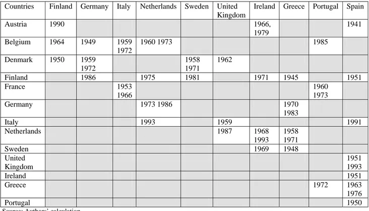
The identification of possible structural changes in data is a current procedure in time series analysis and it assumes an increased relevance in current analysis, as their occurrence makes invalid the results of stationarity tests often used in the analysis of economic convergence. We proceed by applying the Bai and Perron (1998) test to per capita output gaps in each sub-period. The results are reported in Tables 1 and 2 for the sub-periods 1920-2008 and 1950-2008, respectively. No structural changes were found for in the sub-period 1990-2008 due to its reduced dimension. The finding of structural breaks in long time series is in total accordance with the occurrence of events over time that affect the countries’ economic performance with different timings. This evidence reinforces the importance of considering these changes in methodological grounds for evaluating real convergence.

Table 1: Structural changes in per capita output gaps: 1921-2008 Countries Finland Germany Italy Netherlands Sweden United

Kingdom

Ireland Greece Portugal Spain

Austria 1990 1966, 1979 1941 Belgium 1964 1949 1959 1972 1960 1973 1985 Denmark 1950 1959 1972 1958 1971 1962 Finland 1986 1975 1981 1971 1945 1951 France 1953 1966 1960 1973 Germany 1973 1986 1970 1983 Italy 1993 1959 1991 Netherlands 1987 1968 1993 1958 1971 Sweden 1969 1948 United Kingdom 1951 1993 Ireland 1951 Greece 1972 1963 1976 Portugal 1950

Source: Authors’ calculation.

Table 2: Structural changes in per capita output gaps: 1950-2008 Countries Bulgaria Hungary Poland

Austria 1973 Denmark 1988 Finland 1970 France 1962 Netherlands 1965 Sweden 1958 1981 United Kingdom 1973 1964 Ireland 1978 1972 Greece 1958 1988 Spain 1990 1978 Bulgaria 1967 1972

5. Empirical evidence of convergence persistence

Time series notions of convergence imply that per capita output disparities between converging economies follow a stationary process. Therefore, convergence is directly related to the unit root hypothesis in relative per capita output. We use the methodology described in Section 3 to draw conclusions about whether countries are converging or not. The rejection of the null hypothesis of stationary process, I(0), or its rejection in favor to a change from non-stationarity to non-stationarity, ie I(1)-I(0) change, provides evidence of convergence.

We first apply the tests to the Western European countries over the periods 1921-2008. Although this sample is not the focus of the paper, its analysis is relevant to provide evidence about the context of the most developed European Union members and to open the door to the analysis of the trends among the Eastern European countries. In the second subsection we analyze the convergence between EE economies and WE economies using all the available data. In this way, we check the convergence for Bulgaria, Hungary, Poland and Romania over the period 1950-2008 and for Slovakia, Czech Republic, Estonia, Latvia and Lithuania over a shorter period, 1990-2008. In practice, the sample periods are even shorter since the tests ignore 20% of the observations at the beginning and the end of the samples.

5.1 Convergence of Western European economies in the period 1921-2008

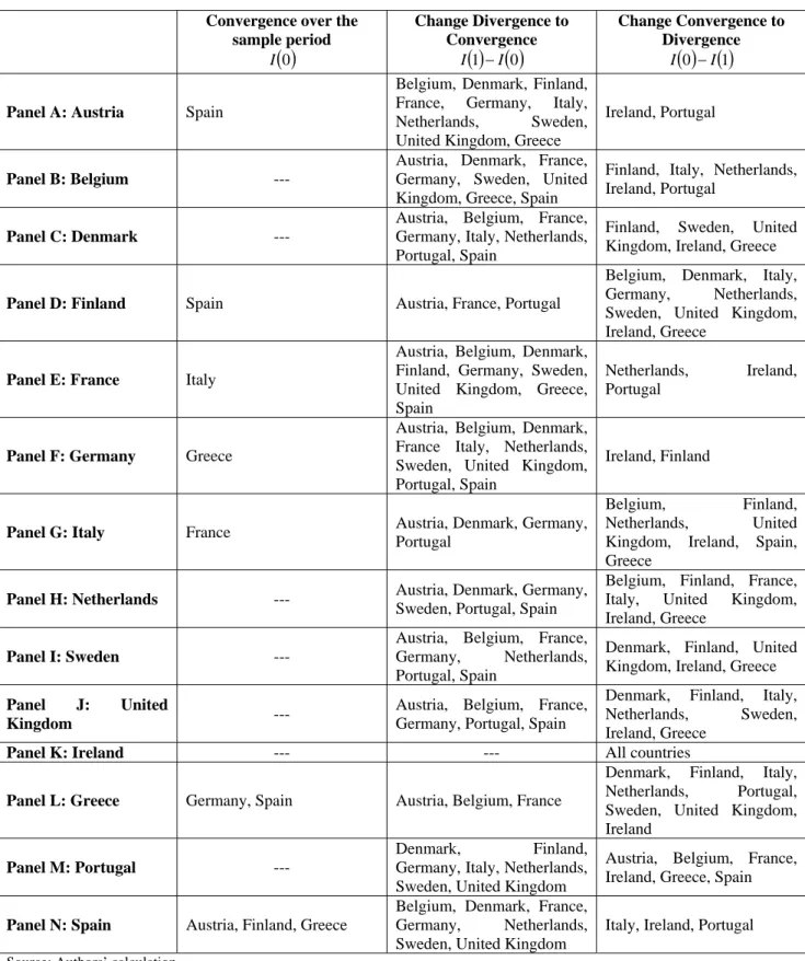
Results of the tests are reported in Table A1 in the Appendix and a summary is provided in Table 3. In general, evidence of no persistence change in favor of the null I(0) hypothesis, was found in 5 series, representing 5.5% of total. For those cases, results suggest that those output gaps follow stationary processes, implying, therefore, convergence of the corresponding countries over the whole sample period. These are the cases of Spain, Austria and Greece; France and Italy, Greece and Germany.

The null I(0) hypothesis was rejected in 86 series. Evidence of I

( ) ( )

0 −I1 changes was detected in 42 series, representing 46.2% of total, which corresponds to cases of economic divergence. Evidence of I

( ) ( )

1 −I 0 changes is present in 44 series, or 48.4% of total, meaning that correspondent countries have begun a catching-up process. Therefore, the results suggest that 49 out of 91 series represent cases of convergence while 42 series represent situations of economic divergence between countries.

The analysis by country is also very informative. Specifically, the analysis reveals that some countries are in better position than others since their output gaps display convergence, ie they follow I

( )

0 processes or present

( ) ( )

1 I 0

I − changes over the sample period with a large number of other countries. These are the cases of Austria and Germany relatively to 11 countries, France and Spain relatively to 10 countries, Belgium relatively to 9 countries, Denmark relatively to 8 countries, Sweden and Portugal relatively to 7 countries, Italy and Greece relatively to 5 countries. Finally, Finland reports convergence with 4 countries and Ireland appears as the only country reporting economic divergence with all countries over the sample period.

Considering that 20% of the observations at the beginning and the end of the sample period are not considered by the tests, in practice, the results are reported to the period 1939-1990. This implies that the economies’ recent performance over the last two decades will not be considered by the results. This issue impacts significantly the results and explains the divergence found in Ireland relatively to the other countries. In fact, Ireland’s catching-up process occurred over the 90s. This also explains the evidence of change from divergence (I(1)) to convergence (I(0)) from Portugal, Spain and Greece relatively to other countries, despite the poor performance of these countries in the last two decades. Regarding the other countries, the results are in accordance to previous literature considering methodological frameworks based on unit roots tests and structural changes in data (see Li and Papell (1999), among others). However, ignoring the occurrence of structural changes in data has led often to the conclusion of lack of convergence (see Bernard and Durlauf, 1995; Fleissig and Strauss, 2001; and Peasaran, 2007, among others).

5.2 Convergence persistence of EE economies relatively to WE economies

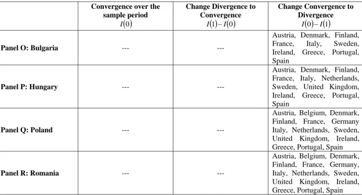
The results of the persistence tests between EE economies and WE economies are reported in Table A2 in the Appendix and a summary is provided in Table 4. In general, the null, I(0) hypothesis has been rejected in favor of

( ) ( )

0 I1

I − changes in the output gap series between WE economies and the group of EE economies formed by Bulgaria, Hungary, Poland and Romania, which suggests a process of economic divergence between these economies and the WE economies over the period 1950-2008, in practice 1962-1996. Only in a very few cases the direction of the change is not clear. These are the cases of the output gaps between Bulgaria and Belgium, Germany, Netherlands and the United Kingdom; also between Hungary, Germany and Belgium. The results for Hungary and Poland are in accordance with the scarce literature covering the eastern European countries (see Bruggemann and Trenkler, 2004).

Table 3: Convergence persistence between Western European economies in the period 1921-2008 Convergence over the

sample period

( )

0 I Change Divergence to Convergence

( ) ( )

1 I 0 I − Change Convergence to Divergence

( ) ( )

0 I1 I −

Panel A: Austria Spain

Belgium, Denmark, Finland, France, Germany, Italy, Netherlands, Sweden, United Kingdom, Greece

Ireland, Portugal

Panel B: Belgium ---

Austria, Denmark, France, Germany, Sweden, United Kingdom, Greece, Spain

Finland, Italy, Netherlands, Ireland, Portugal

Panel C: Denmark ---

Austria, Belgium, France, Germany, Italy, Netherlands, Portugal, Spain

Finland, Sweden, United Kingdom, Ireland, Greece

Panel D: Finland Spain Austria, France, Portugal

Belgium, Denmark, Italy, Germany, Netherlands, Sweden, United Kingdom, Ireland, Greece

Panel E: France Italy

Austria, Belgium, Denmark, Finland, Germany, Sweden, United Kingdom, Greece, Spain

Netherlands, Ireland, Portugal

Panel F: Germany Greece

Austria, Belgium, Denmark, France Italy, Netherlands, Sweden, United Kingdom, Portugal, Spain

Ireland, Finland

Panel G: Italy France Austria, Denmark, Germany,

Portugal

Belgium, Finland, Netherlands, United Kingdom, Ireland, Spain, Greece

Panel H: Netherlands --- Austria, Denmark, Germany,

Sweden, Portugal, Spain

Belgium, Finland, France, Italy, United Kingdom, Ireland, Greece

Panel I: Sweden ---

Austria, Belgium, France, Germany, Netherlands, Portugal, Spain

Denmark, Finland, United Kingdom, Ireland, Greece Panel J: United

Kingdom ---

Austria, Belgium, France, Germany, Portugal, Spain

Denmark, Finland, Italy, Netherlands, Sweden, Ireland, Greece

Panel K: Ireland --- --- All countries

Panel L: Greece Germany, Spain Austria, Belgium, France

Denmark, Finland, Italy, Netherlands, Portugal, Sweden, United Kingdom, Ireland

Panel M: Portugal ---

Denmark, Finland, Germany, Italy, Netherlands,

Sweden, United Kingdom

Austria, Belgium, France, Ireland, Greece, Spain

Panel N: Spain Austria, Finland, Greece

Belgium, Denmark, France, Germany, Netherlands, Sweden, United Kingdom

Italy, Ireland, Portugal

Source: Authors’ calculation.

For the period 1990-2008, in practice 1994-2004, considering a set of EE countries formed by Slovakia, Czech Republic, Estonia, Latvia and Lithuania, the null I(0) hypothesis was rejected for the large majority of the series in favor of an evidence of persistence change. Specifically, I

( ) ( )

1 −I 0 changes in the output gaps between EE economies and WE economies were found in 44 out of 65 series, which is indicative of the catching up process the former economies have undergone. A summary of the results is reported in Table 5.

Latvia and Lithuania are singular cases of convergence in that their output gaps relatively to all WE report a change towards convergence. These economies have moved into a catching up process relatively to WE economies since their output gaps changed from nonstationary to stationary processes. Also Slovakia and the Czech Republic seem to get closer to most WE economies. Slovakia has reduced its distance relatively to a less number of WE economies and

enacted a divergence path relatively to Finland and Ireland. Finally, the results for Estonia suggest clearly I

( ) ( )

0 −I1 changes of the output gap relatively to a set of WE countries like Austria, Finland, Germany, Sweden, Netherlands, Portugal and Italy, while the direction of changes relatively to other WE economies is not clear.

Table 4: Convergence persistence between Eastern European economies and Western European economies in the period 1950-2008

Convergence over the sample period

( )

0 I Change Divergence to Convergence

( ) ( )

1 I 0 I − Change Convergence to Divergence

( ) ( )

0 I1 I − Panel O: Bulgaria --- ---

Austria, Denmark, Finland, France, Italy, Sweden, Ireland, Greece, Portugal, Spain

Panel P: Hungary --- ---

Austria, Denmark, Finland, France, Italy, Netherlands, Sweden, United Kingdom, Ireland, Greece, Portugal, Spain

Panel Q: Poland --- ---

Austria, Belgium, Denmark, Finland, France, Germany Italy, Netherlands, Sweden, United Kingdom, Ireland, Greece, Portugal, Spain

Panel R: Romania --- ---

Austria, Belgium, Denmark, Finland, France, Germany, Italy, Netherlands, Sweden, United Kingdom, Ireland, Greece, Portugal, Spain Source: Authors’ calculation.

Table 5: Convergence persistence between Eastern European economies and Western European economies in the period 1990-2008

Convergence over the sample period

( )

0 I Change Divergence to Convergence

( ) ( )

1 I 0 I − Change Convergence to Divergence

( ) ( )

0 I1 I − Panel S: Slovakia ---

Austria, Belgium, France, Germany, Netherlands, United Kingdom, Greece, Portugal, Spain, Italy

Finland, Ireland

Panel T: Czech

Republic ---

Denmark, Finland, France, Germany, Netherlands, Sweden, Greece, Portugal, Spain, Italy

Austria, Belgium, Ireland

Panel U: Estonia --- ---

Austria, Finland, Germany, Sweden, Netherlands, Portugal, Italy

Panel V: Latvia and

Lithuania ---

Austria, Belgium, Denmark, Sweden, Finland, France, Germany, Italy, Spain, Netherlands, Greece, United Kingdom, Ireland, Portugal,

---

5.3 Convergence persistence between EE economies

The analysis of the convergence between EE economies in the periods 1950-2008 and 1990-2008 is reflected in the results displayed in Table A3 in the Appendix and summarized in Tables 6 and 7, respectively.

As to what concerns the period 1950-2008, there is strong evidence of I

( ) ( )

0 −I1 changes. That is, Bulgaria, Hungary, Poland and Romania have enacted divergence path ways since almost all series changed from stationary to nonstationary processes. The output gap between Bulgaria and Romania is the only case that has not presented evidence of persistence change. Only for a few cases is the direction of change inconclusive. These are the cases of the output gaps of Bulgaria relatively to Belgium, Germany, Netherlands and the United Kingdom; Hungary relatively to Belgium and Germany and Poland relatively to Germany.

Table 6: Convergence persistence between EE economies in the period 1950-2008 Convergence over the

sample period

( )

0 I Change Divergence to Convergence

( ) ( )

1 I 0 I − Change Convergence to Divergence

( ) ( )

0 I1 I −

Panel W: Bulgaria Romania --- Hungary, Poland

Panel X: Hungary --- --- Poland, Romania, Bulgaria

Panel Y: Poland --- --- Romania, Bulgaria, Hungary

Panel Z: Romania Bulgaria --- Hungary, Poland

Source: Authors’ calculation.

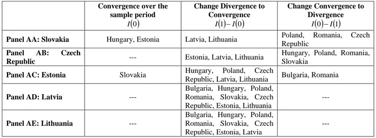
The analysis for the period 1990-2008 considers a larger number of EE economies and reports a general trend of convergence between the economies. That is, I

( ) ( )

1 −I 0 changes of the output gap series are dominant. In particular, Latvia and Lithuania have undergone a catching up process relatively to the other EE economies. Also Estonia has reduced the gap relatively to Hungary, Poland, Czech Republic, Latvia and Lithuania, although it has increased its gap relatively to Bulgaria and Romania. The Czech Republic has also enacted a divergent process relatively to Hungary, Poland, Romania and Slovakia, while this country has also kept an increased distance relatively to Poland and Romania. However, the null I(0) hypothesis is nor rejected for the output gap relatively to Hungary and Estonia.

Table 7: Convergence persistence between EE economies in the period 1990-2008 Convergence over the

sample period

( )

0 I Change Divergence to Convergence

( ) ( )

1 I 0 I − Change Convergence to Divergence

( ) ( )

0 I1 I −

Panel AA: Slovakia Hungary, Estonia Latvia, Lithuania Poland, Romania, Czech

Republic Panel AB: Czech

Republic --- Estonia, Latvia, Lithuania

Hungary, Poland, Romania, Slovakia

Panel AC: Estonia Slovakia Hungary, Poland, Czech

Republic, Latvia, Lithuania Bulgaria, Romania

Panel AD: Latvia ---

Bulgaria, Hungary, Poland, Romania, Slovakia, Czech Republic, Estonia, Lithuania

---

Panel AE: Lithuania ---

Bulgaria, Hungary, Poland, Romania, Slovakia, Czech Republic, Estonia, Latvia

---

Source: Authors’ calculation.

6. Conclusions

The results of this paper suggest that real per capita output gaps between Western European countries seem to follow stationary I

( )

0 processes or, at least, they seem to have switched from non-stationary processes to stationary

( )

0

I processes in most part of the countries. Ireland appears as the only country reporting economic divergence relatively to all countries over the period 1921-2008, since its output gaps have reported changes from stationarity to nonstationarity. The same evidence is reported for the output gaps between Bulgaria, Hungary, Poland and Romania and the Western European economies since the 1950s. However, over the last two decades there has been evidence of changes from non-stationary to stationary processes between the Western European economies and countries belonging to Eastern Europe such as Slovakia, Czech Republic, Latvia and Lithuania. Latvia and Lithuania are singular cases of convergence in that their output gaps relatively to all WE report a change towards convergence. Only Estonia has

demonstrated some difficulties in enacting this catching-up process. Finally, regarding the convergence persistence between Eastern economies, the results suggest generalized changes of per capita output gaps from stationary to non-stationary after the 1950s and general trend to close the gap since the 1990s.

References

Andraz, J. & Rodrigues, P. (2010). Persistence Change in Tourism Data. Tourism Economics, 16(2), forthcoming.

Andrews, D.W.K (1993). Tests for parameter instability and structural change with unknown change point. Econometrica, 61, 821-856.

Andrews, D. W. K. & W. Ploberger (1994). Optimal tests when a nuisance parameter is present only under the alternative. Econometrica, 62, 1383-1414.

Barro, R.& Sala-i-Martin (1991). Convergence across states and regions. Brookings Papers on Economic Activity, 107-182.

Barro, R.& Sala-i-Martin (1991). Convergence. Journal of Political Economy, 100, 223-251.

Barro, R. J. (1991). Economic growth in a cross-section of countries. Quarterly Journal of Economics, 106, 407-443.

Baumol, W. J. (1986). Productivity growth, convergence, and welfare. American Economic Review, 76, 1072-1085.

Belaire-Franch, J. (2005). A proof of the power of Kim's test against stationary processes with structural breaks. Econometric Theory, 21(06), 1172-1176.

Ben-David, D. (1996). Trade and convergence among countries. Journal of International Economics, 40, 279-298.

Bernard, A. & S. Durlauf (1995). Convergence in international output. Journal of Applied Econometrics, 10(2), 97-108.

Bernard, A. & S. Durlauf (1996). Interpreting tests of the convergence hypothesis. Journal of Econometrics, 71, 161-173.

Boreiko, D. (2003). EMU and accession countries: fuzzy cluster analysis of membership. International Journal of Finance and Economics, 8, 309-325.

Busetti, F. & Taylor, A. M. R. (2004). Tests of stationarity against a change in persistence. Journal of Econometrics, 123, 33-66.

DeLong, J. B. (1988). Productivity growth, convergence, and welfare: comment. American Economic Review, 78, 1138-1154.

Evans, P. (1998). Using panel data to evaluate growth theories. International Economic Review, 39, 295-306. Evans, P. & Karras, G. (1996). Convergence revisited. Journal of Monetary Economics, 37, 249-265.

Greasley, D. & Oxley, L. (1997). Time-series based tests of the convergence hypothesis: Some positive results. Economics Letters, 56, 143-147.

Harvey, D. L., S. J. Leybourne & A. M. R. Taylor (2006). Modified tests for a change in persistence. Journal of Econometrics, 134, 441-469.

Holmes, M. J. (2002). Panel data evidence on inflation convergence in the European union. Applied Economics, 9, 155-158.

Kim, J. (2000). Detection of change in persistence of a linear time series. Journal of Econometrics, 95, 97-116. Kim, J. Y., Belaire Franch, J. & Amador, R. (2002). Corringendum to detection of change in persistence of a linear time series. Journal of Econometrics, 109, 389-392.

Kocenda, E. & Papell, D. H. (1997). Inflation convergence within the european union: a panel data analysis. International Journal of Finance and Economics, 2, 189-198.

Kocenda, E. (2001). Macroeconomic convergence in transition countries. Journal of Comparative Economics, 29, 1-23.

Lee, K., Peasaran, M. H. & Smith, R. (1997). Growth and convergence in a multicountry empirical stochastic Solow model. Journal of Applied Econometrics, 12, 357-392.

Levin, R. & Renelt, D. (1992). A sensitivity analysis of cross-country growth regressions. American Economic Review, 82(4), 942-963.

Lucas, R. (1988). On the mechanisms of economic development. Journal of Monetary Economics, 22, 3-42. Lumsdain, R. & D. Papell (1997). Multiple breaks and the unit root hypothesis. The Review of Economics and Statistics, 79(2), 212-218.

Mankiw, N, Romer, D. & Weil, D. (1992). A contribution to the empirics of economic growth. Quarterly Journal of Economics, 107, 407-438.

Mills, T. C. & Holmes, M. J. (1999). Common trends and cycles in European industrial production: exchange rate regimes and economic convergence. Manchester School, 67(4), 557-587.

Peasaran, M. H. (2007). A pair-wise approach to testing for output and growth convergence. Journal of Econometrics, 138, 312-355.

Perron, P. (1989). The great crash, the oil price shock and the unit root hypothesis. Econometrica, 57, 1361-1401.

Quah, D. (1993). Galton´s fallacy and tests of convergence hypothesis. Scandinavian Journal of Economics, 95, 427-443.

Romer, P. (1986). Increasing returns and long run growth. Journal of Political Economy, 94, 1002-1037. Snell, A. (1996). A test of purchasing power parity based on the largest principal component of real exchange rates of the main OECD economies. Economics Letters, 51, 225-231.

Solow, R. (1956). A contribution to the theory of economic growth. Quarterly Journal of Economics, 70, 65-94.

Appendix

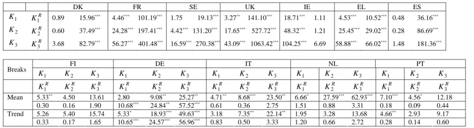
Table A1: Persistence of real convergence in the period 1921-2008 Austria B DK FR DE IT NL SE UK EL PT 1 K R K₁ 0.68 224.74*** _{0.47 63.79}*** _{0.81 155.23}*** _{0.20 140.52}*** _{0.36 4.99}*** _{1.05 11.21}*** _{0.63 27.37}*** _4.36*** _166.39*** _{0.42 5.97}*** _{2.26 1.60} 2 K R K2 0.86 648.97*** 0.35 109.44*** 4.35*** 220.54*** 0.12 283.85*** 0.19 9.90*** 4.30*** 24.95*** 0.51 154.58*** 13.88*** 608.16*** 0.25 15.69*** 5.38*** 1.04 3 K R K₃ 6.62 1305.92*** _{3.25 226.06}*** _15.79*** _449.06*** _{1.71 575.67}*** _{1.05 26.27}*** _15.98*** _57.23*** _{3.80 317.13}*** _{35.16 1224.34}*** _{2.74 39.35}*** _18.45*** _4.53 FI IE ES Breaks 1 K K2 K3 K1 K2 K3 K1 K2 K3 R K₁ K₂R K₃R K₁R K₂R K₃R K₁R K₂R K₃R 2.17 4.12* _14.79* _14.67*** _39.86*** _87.68*** _{2.16 3.66 14.23} Mean 5.54* _9.20** _25.92** _{0.32 0.17 0.88 1.64 1.23 6.74} 1.58 2.71* _12.36* _{2.38 3.47}* _14.66* _{2.16 3.62 14.22} Trend 2.40 2.24 10.14 0.60 0.31 1.06 1.54 1.07 5.90 Belgium DK FR SE UK IE EL ES 1 K _KR 1 0.89 15.96 *** _4.46*** _101.19*** _{1.75 19.13}*** _3.27** _141.10*** _18.71*** _{1.11 4.53}*** _10.52*** _{0.48 36.16}*** 2 K R K₂ 0.60 37.49*** _24.28*** _197.41*** _4.42*** _131.20*** _17.65*** _527.72*** _48.32*** _{1.21 25.45}*** _29.02*** _{0.28 86.69}*** 3 K R K₃ 3.68 82.79*** _56.27*** _401.48*** _16.59*** _270.38*** _43.09*** _1063.42*** _104.25*** _{6.69 58.88}*** _66.02*** _{1.48 181.36}*** FI DE IT NL PT Breaks 1 K K2 K3 K1 K2 K3 K1 K2 K3 K1 K2 K3 K1 K2 K3 R K₁ K₂R K₃R K₁R K₂R K₃R K₁R K₂R K₃R K₁R K₂R K₃R K₁R K₂R K₃R 5.33** _{4.50 13.61 2.80 9.08}** _25.27** _4.71** _8.68*** _23.50** _6.66* _27.59*** _62.93*** _7.10*** _4.56* _12.18 Mean 0.30 0.16 1.90 10.68*** _24.84** _57.52*** _{0.61 0.36 2.75 1.51 0.88 3.31 0.18 0.09 0.44} 5.26 5.40 15.74 5.33* _18.93*** _49.63*** _{3.18 7.35}** _22.14** _{1.95 3.28 13.68 4.66}** _{2.93 9.17} Trend 0.33 0.17 1.65 10.65*** _24.57*** _56.96*** _{0.83 0.50 3.33 1.20 0.66 2.72 0.28 0.14 0.60}

Denmark FR IT NL IE EL PT ES 1 K R K1 1.98 59.19*** 2.80* 32.18*** 0.59 54.40*** 38.95*** 1.37 7.31*** 12.09** 5.53*** 10.16*** 0.70 29.49*** 2 K R K₂ 5.98*** _107.19*** _13.04*** _144.27*** _{0.82 182.28}*** _218.42*** _{3.24 45.12}*** _23.23*** _18.90*** _61.05*** _{0.43 78.46}*** 3 K R K3 18.72***222.29*** 33.97*** 296.51*** 6.77 372.54*** 444.82*** 11.92 98.22*** 54.41*** 44.56*** 130.06*** 2.11 164.90*** FI DE SE UK Breaks 1 K K₂ K₃ K₁ K₂ K₃ K₁ K₂ K₃ K₁ K₂ K₃ R K₁ K₂R K₃R K₁R K₂R K₃R K₁R K₂R K₃R K₁R K₂R K₃R 12.99*** _12.89*** _31.57*** _{1.15 1.92 8.95 11.29}*** _8.52* _21.91** _5.37** _31.83*** _71.62*** Mean 0.12 0.06 0.27 8.91** _8.38** _22.57** _{0.11 0.06 0.23 0.84 0.46 2.87} 13.58*** _13.18** _32.32** _{0.88 1.83 8.94 11.36}*** _8.11** _19.90** _{1.63 1.20 6.94} Trend 0.11 0.06 0.24 7.05** _6.99** _20.22** _{0.11 0.06 0.22 0.90 0.50 3.34} Finland FR IT UK PT 1 K R K₁ 1.11 18.43*** _8.52*** _6.08*** _31.63*** _{1.96 1.96 2.05} 2 K _KR 2 3.38 ** 31.98*** 47.38*** 17.90*** 283.53*** 1.64 1.40 6.89*** 3 K R K₃ 13.82*** _71.94*** _102.10*** _43.77*** _575.05*** _8.24* _{5.77 21.74}*** DE NL SE IE EL ES Breaks 1 K K₂ K₃ K₁ K₂ K₃ K₁ K₂ K₃ K₁ K₂ K₃ K₁ K₂ K₃ K₁ K₂ K₃ R K₁ K₂R K₃R K₁R K₂R K₃R K₁R K₂R K₃R K₁R K₂R K₃R K₁R K₂R K₃R K₁R K₂R K₃R 4.62** _12.43*** _31.75*** _{3.30 6.25}** _19.40** _8.13*** _6.87** _{12.63 117.91}*** _139.16*** _286.29*** _15.28*** _76.50*** _160.97*** _{2.31 1.50 5.54} Mean 1.18 0.90 7.10 0.71 0.39 2.94 0.25 0.13 1.27 0.02 0.01 0.07 1.55 1.34 6.51 0.88 1.47 9.82 3.72** 9.80*** 25.95*** 3.88* 9.13** 25.33** 4.83** 4.51* 14.52* 67.98*** 63.94*** 135.52*** 22.68*** 121.73*** 251.43*** 3.85 2.19 6.54 Trend 1.35 1.01 7.10 0.79 0.44 3.02 0.42 0.22 1.45 0.02 0.01 0.06 0.53 0.30 1.83 0.35 0.19 2.28

France DE NL SE UK IE EL ES 1 K R K1 0.63 224.14*** 7.45*** 0.81 1.36 24.76*** 3.92** 219.93*** 9.17*** 3.99** 0.97 6.63*** 0.85 28.87*** 2 K R K₂ 1.88 355.07*** _17.34*** _{0.69 4.15}*** _128.67*** _22.71*** _21530.45*** _37.74*** _9.51*** _{0.88 22.54}*** _{1.57 89.01}*** 3 K R K3 10.62** 718.11*** 42.38*** 4.42 15.33*** 285.31*** 53.39*** 2930.11*** 83.05*** 25.83*** 5.56 53.05*** 8.85** 185.88*** IT PT Breaks 1 K K₂ K₃ K₁ K₂ K₃ R K₁ K₂R K₃R K₁R K₂R K₃R 1.59 2.32 11.18 3.55* _12.10*** _32.03*** Mean 1.67 1.66 9.64 1.07 0.60 2.40 1.07 0.62 3.12 1.11 0.64 2.80 Trend 1.84 1.69 9.54 1.69 1.09 4.25 Germany IT SE UK IE PT ES 1 K R K₁ 0.75 42.19*** _{1.54 11.96}*** _16.15*** _81.83*** _9.57*** _{2.09 0.76 10.80}*** _{0.29 39.67}*** 2 K _KR 2 1.63 129.16 *** 5.46*** 39.78*** 68.85*** 262.86*** 29.83*** 3.76** 0.92 11.13*** 0.19 110.23*** 3 K R K₃ 9.14** _265.67*** _18.54*** _87.54*** _145.67*** _533.71*** _67.35*** _13.28** _7.20* _29.53*** _{2.56 228.44}*** NL EL Breaks 1 K K₂ K₃ K₁ K₂ K₃ R K₁ K₂R K₃R K₁R K₂R K₃R 3.18** _11.29*** _29.31*** _{1.31 1.65 8.79} Mean 4.46 5.23 15.94 1.87 1.21 5.34 2.52** 11.20*** 29.34*** 1.71 2.17 10.15* Trend 19.38*** _28.92*** _65.56*** _{1.93 1.31 5.39}

Italy SE IE EL PT 1 K R K1 10.43*** 11.40*** 40.17*** 2.89* 2.87* 4.22** 2.29 10.68*** 2 K R K₂ 66.95*** _65.98*** _141.37*** _7.93*** _19.50*** _12.69*** _6.70*** _10.23*** 3 K R K3 141.73*** 139.94*** 289.97*** 22.09*** 46.45*** 33.34*** 19.90*** 25.44*** NL UK ES Breaks 1 K K₂ K₃ K₁ K₂ K₃ K₁ K₂ K₃ R K₁ K₂R K₃R K₁R K₂R K₃R K₁R K₂R K₃R 4.30** _4.50** _15.57** _27.81*** _122.94*** _253.87*** _3.66** _3.00* _10.91 Mean 0.60 0.43 3.63 2.30 33.52*** _75.01*** _{1.42 2.03 9.00} 2.11 2.80*** _11.75* _22.74*** _116.05*** _239.95*** _{1.88 2.31 10.13} Trend 1.12 0.66 3.25 2.89* _44.12*** _96.21*** _{2.41 2.41 8.95} Netherlands SE PT ES 1 K R K₁ 0.49 36.92*** _{1.46 8.36}*** _{0.73 21.41}*** 2 K _KR 2 0.56 36.94 *** 2.75** 52.48*** 0.63 31.62*** 3 K R K₃ 5.21 81.37*** _11.40** _112.93*** _{4.66 68.96}*** UK IE EL Breaks 1 K K₂ K₃ K₁ K₂ K₃ K₁ K₂ K₃ R K₁ K₂R K₃R K₁R K₂R K₃R K₁R K₂R K₃R 4.98*** _26.06*** _60.10*** _9.46*** _28.64*** _64.54*** _5.83** _6.95** _21.81** Mean 3.36 2.58 9.07 0.45 0.24 1.39 0.21 0.11 0.36 5.96*** 32.97*** 73.93*** 1.31 1.36 8.31 5.90 7.08 21.81 Trend 3.99 3.72 11.71 1.63 0.94 3.51 0.39 0.21 1.16 Sweden UK PT ES 1 K R K1 15.50*** 2.09 3.53** 4.82*** 0.35 236.51*** 2 K R K₂ 136.18*** _5.82*** _5.23*** _25.09*** _{0.20 45918.64}*** 3 K R K3 280.34*** 19.53*** 15.66*** 58.15*** 1.63 6152.03*** IE EL Breaks 1 K K₂ K₃ K₁ K₂ K₃ R K₁ K₂R K₃R K₁R K₂R K₃R 119.68*** _307.87*** _623.73*** _14.13*** _60.83*** _129.14*** Mean 0.03 0.02 0.13 2.70 3.28 11.50 36.50*** _27.84*** _61.37*** _19.79*** _95.85*** _199.65*** Trend 0.03 0.02 0.06 0.60 0.35 2.08 United Kingdom IE EL PT 1 K R K₁ 4.63*** _3.56** _80.58*** _38.03*** _5.22*** _11.62*** 2 K _KR 2 12.87 *** 9.57*** 12256.40*** 82.32*** 15.23*** 56.74*** 3 K R K₃ 33.07** _25.96*** _1562.07*** _172.43*** _36.75***_121.45*** ES Breaks 1 K K₂ K₃ R K₁ K₂R K₃R 4.27** _10.74*** _29.45*** Mean 10.61** _69.28*** _146.56*** 6.23*** 10.74*** 29.45*** Trend 2.21 16.81*** _41.61***

Ireland EL PT 1 K R K1 36.39*** 10.77*** 102.11*** 1.87 2 K R K₂ 244.87*** _18.83*** _173.41*** _9.23*** 3 K R K3 497.71*** 43.62*** 354.71*** 25.36*** ES Breaks 1 K K₂ K₃ R K₁ K₂R K₃R 53.09*** _70.67*** _147.93*** Mean 0.14 0.08 0.63 64.04*** _70.45*** _147.93*** Trend 0.05 0.02 0.19 Greece PT ES Breaks 1 K K₂ K₃ K₁ K₂ K₃ R K₁ K₂R K₃R K₁R K₂R K₃R 13.17*** _60.36*** _128.70*** _{1.94 3.37 12.82}* Mean 0.24 0.12 0.47 1.41 0.81 3.04 5.23** _7.42** _21.12** _{0.79 0.46 3.55} Trend 0.34 0.18 0.90 2.74 2.59 10.31 Portugal ES Breaks 1 K K2 K3 R K₁ K₂R K₃R 6.75** _{4.68 13.99} Mean 0.23 0.12 0.74 11.42*** _10.37** _27.13** Trend 0.18 0.09 0.71 Source: Authors’ calculation.

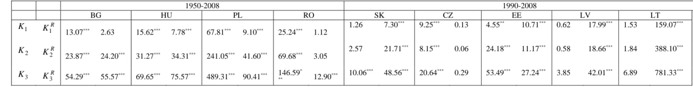
Table A2: Persistence of real convergence of EE economies in the period 1950-2008 and 1990-2008 Austria 1950-2008 1990-2008 HU PL RO SK CZ EE LV LT 1 K R K1 11.61*** 1.56 16.39*** 8.27*** 18.25*** 0.84 0.954 14.97*** 6.01*** 0.20 8.82*** 7.81*** 0.66 14.68*** 1.57 81.01*** 2 K R K₂ 11.23*** _{5.09 62.87}*** _44.56*** _35.23*** _{1.48 1.49 44.56}*** _5.47*** _{0.10 51.54}*** _6.19*** _{0.65 13.46}*** _{1.93 199.75}*** 3 K R K3 27.34*** 15.82 132.95*** 95.74*** 76.68*** 9.13 7.51 94.25*** 14.80*** 0.38 108.21*** 15.72*** 4.13 31.48*** 7.13 404.62*** BG Breaks 1 K K₂ K₃ R K₁ K₂R K₃R 60.99*** _68.37*** _143.22*** Mean 0.22 0.39 5.67 69.83*** _79.48*** _156.62*** Trend 0.09 0.06 0.89 Belgium 1950-2008 1990-2008 BG HU PL RO SK CZ EE LV LT 1 K R K₁ 13.07*** _{2.63 15.62}*** _7.78*** _67.81*** _9.10*** _25.24*** _1.12 1.26 7.30 *** _9.25*** _{0.13 4.55}** _10.71*** _{0.62 17.99}*** _{1.53 159.07}*** 2 K R K₂ 23.87*** _24.20*** _31.27*** _34.31*** _241.05*** _41.60*** _69.68*** _3.05 2.57 21.71 *** _8.15*** _{0.06 24.18}*** _11.17*** _{0.58 18.66}*** _{1.84 388.10}*** 3 K R K₃ 54.29*** _55.57*** _69.65*** _75.57*** _489.31*** _90.41*** 146.59* ** 12.90*** 10.06*** _48.56*** _20.64*** _{0.29 53.49}*** _27.24*** _{3.85 42.01}*** _{6.89 781.33}***

Denmark 1950-2008 1990-2008 BG HU RO SK CZ EE LV LT 1 K R K₁ 63.87*** _{2.08 40.23}*** _6.36*** _28.83*** _0.96 2.13 4.23 2.56 34.82*** 5.79*** 17.19*** 0.84 25.14*** 1.91 535.26*** 2 K _KR 2 119.12 *** 20.21*** 57.79*** 43.90*** 37.90*** 2.88 6.86*** 6.29*** 4.76*** 185.21*** 29.27*** 17.88*** 0.96 25.65*** 2.61 1215.89*** 3 K R K₃ 245.38*** _47.65*** _122.06*** _95.03*** _82.02*** _12.63*** 18.86*** 17.65*** 14.55*** 375.56*** 63.67*** 40.73*** 5.25 54.58*** 8.87 3153.87*** PL Breaks 1 K K₂ K₃ R K1 R K2 R K3 78.60*** _120.60*** _248.28*** Mean 0.36 0.24 2.24 32.50*** _66.28*** _139.77*** Trend 0.37 0.24 2.17 Finland 1950-2008 1990-2008 BG PL RO SK CZ EE LV LT 1 K _KR 1 12.16*** 1.57 65.77*** 6.99*** 25.17*** 0.81 5.06 *** 1.94 11.21*** 34.67*** 7.28*** 3.34 1.03 9.69*** 1.49 130.13*** 2 K R K₂ 16.63*** _10.39*** _112.71*** _24.49*** _39.68*** _{1.22 15.46}*** 2.97 16.99*** 90.69*** 14.35*** 2.57 1.16 9.22*** 1.64 392.48*** 3 K _KR 3 40.31 *** 27.99*** 232.65*** 56.10*** 86.58*** 8.11*** 36.06*** 10.79*** 38.78*** 186.52*** 33.60*** 7.81*** 5.84** 22.77*** 7.23*** 790.09*** HU Breaks 1 K K₂ K₃ R K₁ K₂R K₃R 53.36*** 51.82*** 110.73*** Mean 0.17 0.10 1.37 47.46*** _40.49*** _86.48*** Trend 0.08 0.04 0.56

France 1950-2008 1990-2008 HU PL RO SK CZ EE LV LT 1 K R K₁ 33.47*** _5.87*** _313.29*** _{3.01 83.87}*** _{0.64 2.02 6.22}*** 2.20 6.16*** 3.73 11.39*** 0.72 17.66*** 1.74 196.84*** 2 K _KR 2 62.90 *** 37.18*** 221.40*** 9.69*** 130.03*** 1.11 6.28*** 18.50*** 3.60 11.89*** 17.11*** 14.79*** 0.70 19.13*** 2.18 458.12*** 3 K R K₃ 132.92*** _81.54*** _1668.64*** _24.76*** _267.28*** _7.87*** 17.67*** 42.12*** 12.14*** 28.87*** 39.35*** 34.63*** 4.11* 43.14*** 7.92*** 921.36*** BG Breaks 1 K K₂ K₃ R K₁ K₂R K₃R 119.74*** _119.01*** _244.94*** Mean 0.07 0.04 1.31 161.07*** _181.35*** _369.39*** Trend 0.06 0.04 1.19 Germany 1950-2008 1990-2008 BG HU PL RO SK CZ EE LV LT 1 K R K₁ 6.35*** _{1.31 5.30}** _{1.96 9.82}*** _8.00*** _81.29*** _{0.73 0.83 33.17}*** _{1.04 6.94}*** _463.74*** _8.23*** _{0.74 14.21}*** _{2.13 65.83}*** 2 K _KR 2 5.38 ** 10.22*** 5.76** 6.13*** 44.25*** 28.69*** 110.51*** 1.07 1.08 105.41*** 0.98 9.26*** 1253.42*** 7.16*** 0.85 13.15*** 3.04 168.71*** 3 K R K₃ 15.89*** _27.66*** _18.43*** _18.13*** _95.73*** _1101.51*** _1648.19*** _7.71*** _6.30*** _215.95*** _5.49** _23.58*** _6024.07*** _18.74*** _5.23** _30.33*** _9.74*** _342.55*** Italy 1950-2008 1990-2008 BG HU PL RO SK CZ EE LV LT 1 K R K₁ 38.95*** _{1.11 65.32}*** _3.62 80.33** * 4.07 44.46*** 0.59 1.67 7.46*** _{2.03 9.93}*** _9.81*** _11.46*** _{0.83 17.50}*** _{2.07 216.33}*** 2 K R K₂ 57.41*** _8.38*** _79.26*** _23.41*** 208.94** * 10.41*** 136.37*** 0.93 4.10 21.83*** _{2.71 21.25}*** _56.35*** _13.51*** _{0.93 18.55}*** _{2.83 523.95}*** 3 K R K₃ 121.99*** _23.98*** _165.72*** _53.77*** 425.10** * 27.71 *** _179.95*** _7.30*** 13.28*** 48.79*** 10.11*** 47.63*** 117.84*** 31.89*** 5.09** 42.07*** 8.93 1053.02

Netherlands 1950-2008 1990-2008 BG PL RO SK CZ EE LV LT 1 K R K₁ 9.64*** _{1.26 44.10}*** _{4.61 186.13}*** _0.62 2.30 21.09*** 6.02*** 0.31 12.44*** 5.70** 1.17 11.54*** 2.69 57.57*** 2 K _KR 2 7.49 *** 9.26*** 85.98*** 13.66*** 290.86*** 1.23 7.58*** 73.59*** 7.22*** 0.17 66.04*** 4.64* 1.62 10.93*** 4.11 152.82*** 3 K R K₃ 19.57*** _25.74*** _179.18*** _33.21*** _588.93*** _8.47*** 20.29*** 152.31*** 19.34*** 1.11 137.22*** 12.48*** 6.63*** 25.86*** 11.70*** 310.77*** HU Breaks 1 K K2 K3 R K₁ K₂R K₃R 65.11*** _75.39*** _156.54*** Mean 0.16 0.10 1.41 85.23*** _1107.12*** _221.44*** Trend 0.12 0.07 1.09 Sweden 1950-2008 1990-2008 HU RO SK CZ EE LV LT 1 K R K1 17.133*** 4.52 21.89*** 0.71 1.89 1.69 2.77 21.88*** 7.38*** 9.55*** 0.80 17.54*** 1.80 405.86*** 2 K R K₂ 27.42*** _24.38*** _27.94*** _{1.19 3.46 1.33 2.73 104.03}*** _37.10*** _11.57*** _{0.82 18.60}*** _{2.24 1345.45}*** 3 K R K3 60.21*** 55.66*** 63.10*** 8.11*** 11.94*** 5.99** 8.93*** 213.20*** 79.33*** 28.19*** 4.37 41.35*** 7.85 2468.68*** BG PL Breaks 1 K K₂ K₃ K₁ K₂ K₃ R K₁ K₂R K₃R K₁R K₂R K₃R 143.79*** _178.13*** _363.46*** _32.36*** _43.22*** _93.67*** Mean 0.08 0.05 1.71 0.18 0.09 1.02 124.62*** _151.35*** _309.84*** _61.35*** _139.02*** _285.26*** Trend 0.09 0.06 1.94 0.11 0.06 0.56

United Kingdom 1950-2008 1990-2008 BG RO SK CZ EE LV LT 1 K R K₁ 17.36*** _{3.73 104.75}*** _1.75 2.58 4.79 3.35 0.33 4.35 12.53*** 0.74 19.12*** 1.21 307.20*** 2 K _KR 2 23.40 *** 36.29*** 156.97*** 6.53*** 7.37*** 15.82*** 2.28 0.17 11.02*** 15.85*** 0.74 21.08*** 1.32 184.65*** 3 K R K₃ 53.99*** _79.79*** _321.17*** _20.23*** 19.86*** 36.76*** 7.67*** 0.83 26.17*** 36.71*** 4.29 47.17*** 6.23*** 1034.42*** HU PL Breaks 1 K K₂ K₃ K₁ K₂ K₃ R K1 R K2 R K3 R K1 R K2 R K3 105.65*** _119.87*** _246.75*** _299.78*** _462.43*** _932.09*** Mean 1.09 2.57 10.72 0.41 0.28 2.04 117.61*** _133.88*** _273.62*** _390.58*** _557.55*** _1122.31*** Trend 0.28 0.22 2.76 0.44 0.31 2.20 Ireland 1950-2008 1990-2008 HU RO SK CZ EE LV LT 1 K _KR 1 29.50*** 3.57 97.31*** 0.89 9.35 *** 0.49 12.01*** 0.95 23.32*** 17.74*** 2.34 26.20*** 5.32** 76.57*** 2 K R K₂ 68.42*** _29.26*** _283.08*** _2.02 36.76*** 0.27 23.45*** 0.72 89.38*** 25.28*** 4.65 46.31*** 9.25*** 116.07*** 3 K _KR 3 143.75 *** 65.74*** 573.39*** 10.58*** 78.66*** 1.42 52.03*** 3.63 183.88*** 55.65*** 15.78*** 97.75*** 23.10*** 237.22*** BG PL Breaks 1 K K₂ K₃ K₁ K₂ K₃ R K₁ K₂R K₃R K₁R K₂R K₃R 69.58*** 57.86*** 122.43*** 38.11*** 41.85*** 90.17*** Mean 0.08 0.05 1.37 0.12 0.06 0.57 58.68*** _50.89*** _108.74*** _43.05*** _39.99*** _86.38*** Trend 0.03 0.01 0.21 0.05 0.02 0.15

Greece 1950-2008 1990-2008 BG RO SK CZ EE LV LT 1 K R K₁ 4.67* _{0.53 33.70}*** _{0.20 1.00 9.11}*** 1.08 3.62 5.37* 9.14*** 0.41 14.95*** 1.12 145.65*** 2 K _KR 2 3.32 1.12 55.88 *** 0.13 1.12 40.48*** 0.69 7.33*** 30.87*** 11.04*** 0.30 15.09*** 1.13 216.91*** 3 K R K₃ 10.63*** _8.49*** _118.98*** _2.18 6.33*** 86.09*** 3.46 19.76*** 66.87*** 27.09*** 2.37 34.72*** 5.39* 438.94*** HU PL Breaks 1 K K₂ K₃ K₁ K₂ K₃ R K1 R K2 R K3 R K1 R K2 R K3 25.28*** _20.40*** _45.70*** _72.35*** _111.14*** _229.50*** Mean 0.40 0.28 2.35 0.12 0.06 0.56 19.64*** _19.22*** _44.92*** _9.02*** _8.47*** _23.76*** Trend 0.41 0.28 2.32 0.16 0.08 0.54 Portugal 1950-2008 1990-2008 BG HU PL RO SK CZ EE LV LT 1 K _KR 1 _18.43*** _{0.84 27.15}*** _{1.97 152.47}*** _{1.318 24.51}*** _{0.45 2.19 9.41}*** _{2.64 5.80}** _2413.33*** _7.28*** _{1.64 12.93}*** _5.25** _95.87*** 2 K _KR 2 _36.49*** _{4.13 75.60}*** _15.51*** _3451.50*** _{2.404 46.18}*** _{0.55 6.26}*** _36.38*** _{4.92 11.40}*** _3514.12*** _7.76*** _{3.38 12.85}*** _10.79*** _215.74*** 3 K _KR 3 80.11*** 15.43*** 157.31*** 38.23*** 2391.55*** 9.057*** 99.58*** 5.71* 17.64*** 77.89*** 14.89*** 27.91*** 3137.50*** 20.21*** 11.59*** 30.09*** 26.41*** 436.60*** Spain 1950-2008 1990-2008 HU RO SK CZ EE LV LT 1 K R K₁ 3.54 7.22*** _25.34*** _{0.46 1.49 3.61 1.77} 17.58*** 12.99*** 10.67*** 0.74 16.93*** 2.09 331.91*** 2 K _KR 2 3.31 30.87 *** 123.87*** 0.50 2.78 6.93*** 1.77 47.68*** 78.00*** 14.58*** 0.74 18.60*** 2.96 1450.60*** 3 K R K₃ 11.86*** _67.72*** _254.95*** _5.22* 10.51*** 18.97*** 7.52*** 99.74*** 161.14*** 34.23*** 4.36 42.17*** 9.98*** 1690.56***

BG PL Breaks 1 K K₂ K₃ K₁ K₂ K₃ R K₁ K₂R K₃R K₁R K₂R K₃R 13.59*** _8.32*** _20.91*** _36.01*** _39.56*** _84.82*** Mean 0.09 0.05 0.71 0.13 0.07 0.76 20.39*** _13.17*** _30.21*** _39.40*** _39.62*** _84.82*** Trend 0.09 0.05 1.02 0.11 0.06 0.56 Source: Authors’ calculation.