M
ASTER
M
ONETARY AND
F
INANCIAL
E
CONOMICS
M
ASTER
’
S
F
INAL
W
ORK
D
ISSERTATION
C
ONTAGION IN
EU
S
OVEREIGN
Y
IELD
S
PREADS
A
NA
C
ATARINA
R
AMOS
F
ÉLIX
M
ASTER IN
M
ONETARY AND
F
INANCIAL
E
CONOMICS
M
ASTER
’
S
F
INAL
W
ORK
D
ISSERTATION
C
ONTAGION IN
EU
S
OVEREIGN
Y
IELD
S
PREADS
A
NA
C
ATARINA
R
AMOS
F
ÉLIX
S
UPERVISION:
ANTÓNIO
A
FONSOi
Contagion in EU Sovereign Yield Spreads
Ana Catarina Ramos Félix*
†School of Economics and Management
Technical University of Lisbon
Supervisor: António Afonso
30
thSeptember 2013
__________________
I am very grateful to António Afonso to his support and comments. I also thank my parents, my sister
Carla and Hugo Moutinho for their support and advices.
†
ii
Abstract
Since the beginning of the sovereign debt crisis in the Euro Area, the main concern for the European leaders is to prevent against the possible contagion from the distress countries, as Greece, Ireland and Portugal. In our research, we will try to understand if there is a spillover effect from the countries mentioned before and which determinants can be considered as a mechanism of transmission of the sovereign debt crisis. We will perform an econometric analysis in a panel of 13 EU countries (Austria, Belgium, Denmark, Finland, France, Greece, Ireland, Italy, the Netherlands, Portugal, Spain, Sweden and the United Kingdom), covering the period 2000:Q1 to 2013:Q1, and after we analyze each country individually, on the basis of a SUR analysis. We find that the countries with deteriorated macro and fiscal fundamentals are more vulnerable to contagion and are more affected by the international, liquidity and credit risks.
iii
Contents
1. Introduction... 1
2. Literature Review ... 3
2.1. Sovereign yield determinants and involved risk factors ... 3
2.2. Contagion... 6
3. Data and Variables... 9
4. Empirical Analysis... 11
4.1. Panel estimation results ... 11
4.2. Robustness ... 19
4.3. Country estimation - SUR ... 22
5. Conclusion ... 32
References... 34
1
1. Introduction:
Following the collapse of the Lehman Brothers, in September 2008, and the intensification of the international financial crisis in 2008-2009, fiscal imbalances increased in several countries in the Euro Area and the long-term government bond yields rose relative to the German Bund, after a period about 10 years of apparently stability at very low levels. The first phase of the crisis was associated to the global uncertainty and the high fiscal cost of the measures taken by the Irish government to rescue the largest Irish banks. These developments might have played a key role in the evolution of the Euro Area and initiated the sovereign debt crisis. The situation started to improve in Spring 2009, but after the announcement of the Greek Prime Minister disclosing the bad fiscal position of the country, the revised budget deficit was the double of the previous estimate, the sovereign spreads increased markedly, engulfing the whole European Union (EU) and Monetary Union to the biggest crisis since the creation of the Economic and Monetary Union (EMU). As the crisis advanced, the macroeconomic fundamentals deteriorated and the accumulated budget deficits became a problem, with countries implementing fiscal measures to reverse the situation.
2
intervened to help Greece, which was the first country to be financially rescued. The European Central Bank (ECB) used a series of unprecedented measures to stabilise the financial system by providing liquidity both in the short-term and in the long-term and by lowering the main policy rate. The ECB also expanded the maximum maturity for refinancing and extended the collateral list.
The countries with more solid fiscal fundamentals, such as Austria, Finland and the Netherlands, also witnessed a rising in their spreads relative to the German Bund, but none of the market participants suggested that the developments in sovereign bond yields required re-assessment of the respective government credit risk. As opposed to the peripheral countries, the so-called core countries did not suffer credit rating downgrades and kept the triple-A classification.
In this study, we investigated the possible spillover effects between the peripheral countries and if this effect could be spreading to the other countries with more solid macroeconomic and fiscal fundamentals, inside and outside the Euro Area. The consensus in the literature identified three factors affecting sovereign bond yields. First, the aggregate risk associated to changes in monetary policy, as well as to the global risk aversion and uncertainty. Second, the country-specific risk affected the ability to raise funds in the primary market and undermined liquidity in the secondary market. The country-specific risk could come from worsening fundamentals or indirectly via spillover effects and could be related to changes in default probabilities on sovereign debt. Finally, the contagion risk from Greece could have spread to other EMU countries, notably Portugal and other peripheral countries.
3
panel data of 13 EU countries (Austria, Belgium, Denmark, Finland, France, Greece, Ireland, Italy, the Netherlands, Portugal, Spain, Sweden and the United Kingdom) covering the period from 2000-Q1 to 2013-Q1. We studied the entire panel and then we performed an individual analysis for each country based on the SUR methodology.
We can summarize shortly some conclusions of our study: the global risk aversion had an important impact in the sovereign debt crisis, suggesting than the investors were more sensitive to the market sentiment and to the behaviour of the public debt ratio. Moreover, we also identified an important spillover effect between the yield spreads in the EMU countries.
This study is organised as follows. Section two covers the related literature. Section three explains and discusses the data and the construction of the variables. Section four presents the methodology and the results. Finally, section five summarizes the conclusions.
2. Literature Review
2.1. Sovereign yields determinants and involved risk factors:
A large empirical literature has studied the main determinants of sovereign spreads. After a period of stability, where the literature investigated the convergence in sovereign bond yields, the literature has focused on understanding the fast divergence and the main explanatory variables for the sovereign spreads.
4
normally estimated using indicators of past or projected fiscal performance. Finally, the last potential risk factor is the liquidity risk. The risk refers to the need of having large and deep bond markets, where it is easier for the investors to find a counterpart and carry out trades whenever they want to. Usually, in liquid markets, the prices do not change much due to individual transactions. These reasons explain why the investors will require a smaller premium, in other words the extra interest rate an investor ask for bearing the liquidity risk. Typically, the liquidity risk is approximated by the bid-ask spread, but it is still particularly difficult to evaluate empirically.
In the literature, the conclusions regarding the influence of the three risk factors described above are not unanimous. First, the global risk aversion was considered an important determinant of bond yield spreads during the period prior to 2007, as mentioned by Barrios et al. (2009), Sgherri and Zoli (2009) and Favero et al. (2010). On the other hand, Arghyrou and Kontonikas, as well as Favero and Missale (2011), concluded that the market did not price the international risk factor before the beginning of the international crisis, so the global risk aversion just started to play an important key role, after the collapse of the Lehman Brothers. The effect was more pronounced during periods of uncertainty in international financial conditions (Barrios et al., 2009) and when the macroeconomic and fiscal fundamentals become more vulnerable (De Santis, 2012).
5
Finally, the liquidity risk is the more disputed factor in the literature. Some authors, as Bernoth et al. (2004), Pagano and Von Thadden (2004) and Jankowitsch et al. (2006), concluded that liquidity has a limited role as determinant of sovereign yield spreads. On the other hand, for Bernoth et al. (2009), the liquidity risk was an important factor to explain the yield spreads. During periods of financial turbulence with higher and more volatile interest rates, the investors are willing to pay lower yields for higher sovereign debt liquidity.
Another important point of consensus in the literature is the importance of macroeconomic and fiscal fundamentals in a country. The existing studies divide the EMU countries into two categories: core and peripheral (Greece, Portugal, Ireland and Spain) countries (see e.g. De Santis, 2012). During the sovereign debt crisis in the Euro Area, the peripheral countries were more affected by the sovereign solvency risk and also more exposed to spillover effects, as suggested by the studies of Arghyrou and Kontonikas (2011), De Santis (2012) and Giordano et al. (2012). This fact was supported by their feeble economies and fiscal fragilities, generating a revision of market expectations and an increase on spreads in these countries. Arghyrou and Kontonikas (2011) and Caceres et al. (2010) concluded for the importance of the implementation of credible reforms for peripheral countries to improve notably debt public management and external competitiveness.
On the other hands, countries with solid fiscal fundamentals, as Austria, Finland and the Netherlands, were not affected by contagion (Giordano et al., 2012), but according to the findings of De Santis (2012), the spreads of these countries depended largely on the demand of German Bunds, during the crisis. In other words, when the
6
also higher, so, it implies that the spreads will become more stable when the regional financial turbulence ceases and risk aversion returns to normality.
At the UE level, Arghyrou and Kontonikas (2011), De Santis (2012) and Caceres et al. (2010) suggested that the authorities have an important key role to ensure the stability of the Euro Area financial system, developing effective mechanisms of supervision and policy coordination.
Therefore, our empirical analysis will consider as determinants of the 10-year governments bonds yields the GDP real growth rate, the budget balance-to-GDP ratio, the public debt-to-GDP ratio, the balance of payment as a percentage of GDP, the real effective exchange rate, the international risk (represented by the VIX: the S&P 500 implied stock market volatility), and the bid-ask spread.
2.2. Contagion:
7
In the literature, we can find several definitions of contagion, Pericoli and Sbracia (2003) summarized the most five commons facts to describe contagion effects: 1) when a country is affected by the crisis, the probability to spread to another country rises sharply, 2) the volatility of asset prices from the crisis country reaches the financial markets of other countries, 3) a significant increase in co-movements of asset prices is conditional to a crisis occurring in other market, 4) the transmission mechanisms of financial assets increases significantly and 5) if a country is affected by the crisis, it can lead to changes in co-movements of asset prices in other countries due to changes in mechanisms of transmission between the countries.
8
Reference: Methodology: Main results:
Sovereign Spreads: Global Risk Aversion,
Contagion or
Fundame ntals?
Carlos Caceres, Vincenzo Guzzo and Miguel Segoviano (2010)
The model used in the analysis of the determinants of sovereign swap spreads is described by GARCH (1, 1) specification. The model is described using two equations. The first equation is the mean equation for the swap spread as a function of explanatory variables, including the Index of Global Risk Aversion (IGRA), Spillover Coefficient (SC), balance as %GDP and debt to GDP ratio. The second is the conditional variance as a function of the lag of squared residual from the mean equation (ARCH term) and last period variance (GARCH term).
The authors found that the distress dependence for each period crisis shows that the causes of contagion can be found among the countries affected by the financial crisis. During the sovereign crisis, the increase in country-specific risks, directly by worsening in fundamentals or indirectly by spillovers from other sovereigns lead to a number of policy implications. The link between debt management and financial stability suggest the need for a closer coordination with monetary and financial authorities.
The EMU sovereign debt crisis:
Fundame ntals, expectations and contagion
Michael G. Arghyrou and Alexandros Kontonikas (2011)
The authors want to model the spreads before and after the crisis. Therefore, they employed a baseline model for spreads relating country-specific macroeconomic fundamentals, using the logarithm of the real effective exchange rate, the VIX to denote the international risk factor and the noise. They extent their model using a vector of explanatory variables, including liquidity risks, output growth differential, expected budget balance and expected gross debt differential.
To analysis the period during the crisis, the authors included also the spread of the benchmark country, in this case, Germany.
The authors concluded that there was a period of convergence trade before the crisis , but some countries displayed a clear deterioration of their macroeconomics fundamentals. They identified three reasons to explain these results: liquidity risk, expectations that peripheral EMU countries growth with Euro and lack of mechanism establishing credibility.
The findings lead to policy implications both at union and national level.
Sovereign risk, European crisis resolution policies and bond yields
Juha Kilponen, Helinä Laakkonen and Jouko Vilmunen (2012)
For their analysis, the authors studied the determinants of sovereign yields using the Ordinary Least Squares estimation method for the countries in their sample. The parameters which described the contagion effects are CDS, bid-ask spreads, VIX and ITRX (proxy for general risk atmosphere in the European debt market). The other explanatory variables capture the impact of different policies and risk factors.
The findings showed that many decisions to stabilize the European debt crisis have a significant impact in the sovereign yield spreads, at least in the short-run, depending on country-specific conditions, the decisions caused different reactions which can lead to contagion. The contagion can be reflected by the decision that causes. However, the policy decisions have been a stabilizing effect.
The determinants of sovereign bond yield spreads in the EMU
António Afonso, Michael G. Arghyrou and Alexandros Kontonikas (2012)
The authors employed the Two-Stage Least Squares (2SLS) method to explain the 10-year government bond yield spread vers us Germany in function of international risk factor, bond market liquidity conditions, macro – and fiscal fundamentals and contagion effects incorporating country-specific risks.
9
3. Data and Variables:
For our study, we use a panel of 13 countries: Austria (AT), Belgium (BE), Denmark (DN), Finland (FI), France (FR), Greece (GR), Ireland (IR), Italy (IT), the Netherlands (NL), Portugal (PT), Spain (SP), Sweden (SW) and the United Kingdom (UK).
The 10-year government bond yields (yield), the real growth rate of GDP (GDP), the public debt-to-GDP ratio (Debt), the budget balance to-GDP ratio (Budget) and the real effective exchange rate (REER) are taken from Eurostat website. The bid-ask spread (BID) variable was provided by the European Central Bank, the VIX (VIX) by the CBOE website and the current account balance-to-GDP ratio (BOP) was obtained from the Data Market website (the source being Eurostat).
Initially, we considered the use of monthly data, but for some variables, as GDP, such data are not available. Therefore, we opted for the use of quarterly data. The 10-year government bond yields and the real effective exchange rates ate initially monthly and we had to calculate the respective quarterly average. We used the same procedure for the daily values of the VIX and bid-ask spread data.
Our dependent variable is the yield spread of the countries mentioned before, which is the difference between the yields of the observed country and the yield of the benchmark country, in our case, Germany.
10
budget balance should cause a reduction (increase) in the spreads, the same reasoning for the current account balance, while if we expected a higher (lower) public debt, we should see increasing (reducing) spreads.
The real effective exchange rate denotes the variable usually used to capture the
credit risk from macroeconomic disequilibrium. We used the “Real effective exchange
rate - 41 trading partners - Index (2005 = 100)” from Eurostat in which an increase of
this index represents a loss of competitiveness. In practice, we have computed the
variation of the real effective exchange rate. Therefore, a positive (negative) variation of
the real effective exchange rate describes an appreciation (depreciation) of the currency and, according to Arghyrou and Kontonikas (2011), it should cause an expected increase (decrease) in the spreads.
The VIX (the logarithm of the S&P 500 implied stock market volatility index) is generally used as proxy for the international risk factor. When we expect a higher (lower) value for the international risk, then the lower (higher) is the confidence of investors in the international market, and they would require a higher (lower) return for the same government bond yield, so the spreads should increase (decrease).
11
4. Empirical analysis
4.1. Panel estimation results
Baseline
We start by using a panel data approach, using a unified framework of analysis to obtain the aggregate effect of the main variables on the sovereign spreads. The baseline specifications are as follow:
(1) = β0 + β1* + β2.* i,t+ β3*vixt+ β4*bidi,t + j,t*
(2) = α0 + α1* + α2.* i,t+ α3*vixt+ α4*bidi,t + i,t*
(3) = β0 + β1* + β2.* i,t+ β3*vixt+ β4*bidi,t + j,t*
(4) = α0 + α1* + α2.* i,t+ α3*vixt+ α4*bidi,t + j,t*
Where i≠j and ={GDP, Budget, Debt, BOP, REER} is the vector of the main determinants of the sovereign yield spreads. ∆yield is the variation of each country’s
yields. Model (1) includes the possible spillover effects of the spreads in t-1; model (2) contains the effect of the variation of the yields in t-1; models (3) and (4) follow the same idea as models (1) and (2), respectively, but in period t.
As we mentioned before, regarding the variable REER, we used the quarterly-on-quarterly variation (comparing, for instance, the real effective exchange rate index of 2000Q1 with the real effective exchange rate index of 2000Q2). Due to the correlation between the Budget and ΔDebt, we never include them in the same regression at the same time.
12
the possible contagion effect only including EMU countries. In addition, we have also included Denmark, Sweden and the United Kingdom to test the robustness of our results.
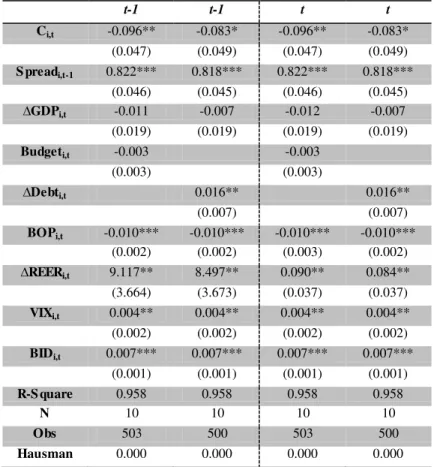
First of all, we only test the impact of the main determinants of sovereign spreads that we might call as core variables (see appendix A1). In this case, we perform the Hausman's test, to verify if it is more appropriate to use fixed or random effects. Random effects are only adequate when there is a reasonable guarantee that the individual effects are not correlated with the variables taken as regressors, therefore we only apply this test when we study the impact of the core variables. When we include the spreads and the variation of the yields in the model, the variables are correlated. The null hypothesis is the non-existence of correlation, meaning random effects should be used. Then, when the p-values are higher than 0.10, we don't reject the null hypothesis and for p-values lower than 0.10, we consider fixed effects.
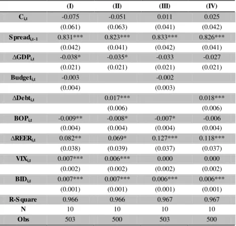
In Table I, we report the results of the estimation for the spreads of 10-year government bond yields: columns (I) and (II) report the results for the model (1), and columns (III) and (IV) for model (2).
13
decrease in the spread of 0.008 p.p., on average. The bid-ask spread has a significant impact on the spreads, although of a limited magnitude. The VIX and the real GDP growth rate have an upward and downward effect, respectively, on spreads in model (1), 0.007 for the VIX and 0.037 p.p. for GDP, both in average. The budget balance does not come across as statistically significant.
Table I - Estimation results for the determinants of 10-year yields spread: models (1) and (2)
(I) (II) (III) (IV)
Ci,t -0.075 -0.051 0.011 0.025
(0.061) (0.063) (0.041) (0.042)
S preadi,t-1 0.831*** 0.823*** 0.833*** 0.826***
(0.042) (0.041) (0.042) (0.041)
∆GDPi,t -0.038* -0.035* -0.033 -0.027
(0.021) (0.021) (0.021) (0.021)
Budgeti,t -0.003 -0.002
(0.004) (0.003)
∆Debti,t 0.017*** 0.018***
(0.006) (0.006)
BOPi,t -0.009** -0.008* -0.007* -0.006
(0.004) (0.004) (0.004) (0.004)
∆REERi,t 0.082** 0.069* 0.127*** 0.118***
(0.038) (0.039) (0.037) (0.037)
VIXi,t 0.007*** 0.006*** 0.000 0.000
(0.002) (0.002) (0.002) (0.002)
BIDi,t 0.007*** 0.007*** 0.006*** 0.006***
(0.001) (0.001) (0.001) (0.001)
R-S quare 0.966 0.966 0.967 0.967
N 10 10 10 10
Obs 503 500 503 500
Note: the asterisks *, ** and *** represent significance at 10, 5 and 1% level, respectively. The values between parentheses are the standard errors. N is the
number of countries included in the sample and Obs is the number of observations.
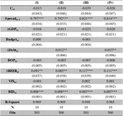
Table II presents results for the models including the potential contagion spreads and the variations of the yields at period t: columns (I) and (II) refer to model (3) and columns (III) and (IV) refer to model (4).
14
above, increase spreads in 0.014 p.p. and 0.101 p.p. respectively, on average. The bid-ask spread is also statistically significant inducing an increase in the spreads of 0.008. In this case, the real GDP growth rate and the balance of payment ratio have no impact on the 10-year yield spreads. As previously, the budget balance is not significant.
Table II - Estimation results for the determinants of 10-year yields spread: models (3) and (4)
(I) (II) (III) (IV)
Ci,t -0.013 -0.010 -0.039 -0.026
(0.043) (0.046) (0.044) (0.047)
S preadi,t-1 0.797*** 0.792*** 0.821*** 0.814***
(0.034) (0.033) (0.046) (0.045)
∆GDPi,t -0.016 -0.013 -0.025 -0.020
(0.021) (0.021) (0.021) (0.021)
Budgeti,t 0.000 -0.001
(0.004) (0.004)
∆Debti,t 0.012** 0.015**
(0.006) (0.006)
BOPi,t -0.003 -0.003 -0.007 -0.006
(0.005) (0.005) (0.005) (0.005)
∆REERi,t 0.091** 0.085** 0.117*** 0.111***
(0.037) (0.038) (0.039) (0.040)
VIXi,t -0.001 -0.001 0.002 0.001
(0.002) (0.002) (0.002) (0.002)
BIDi,t 0.008*** 0.008*** 0.007*** 0.007***
(0.001) (0.001) (0.001) (0.001)
R-S quare 0.969 0.969 0.948 0.965
N 10 10 10 10
Obs 503 500 503 500
Note: the asterisks *, ** and *** represent significance at 10, 5 and 1% level, respectively. The values between parentheses are the standard errors. N is the
number of countries included in the sample and Obs is the number of observations.
Therefore, our results indicate that the models with spread contagion in t-1 highlight the impact of some determinants of EMU countries. This fact may be reflected the importance of sovereign government yields' behaviour, affecting the expectations of economic agents.
15
builds his expectations, he will be aware of the evolution of the sovereign yields relative to the German bonds. In capital markets, if there are no improvement indicators for a specific country, the spread at this time will be tightly correlated with the previous value.
Additionally, the public debt ratio has a significant impact on the 10-year yield spreads, in both periods (on average, 0.016 p.p.). A worsening in the public debt ratio affects the country's probability of default and discourages investments. As a consequence, the countries have to borrow outside, from other countries or institutions, deteriorating their economic situations and affecting negatively the spreads. For instance, the impact of the bid-ask spreads (on average, 0.008 p.p.) is strongly significant reflecting that the investors required a greater premium for bearing a liquidity risk.
The variation of the real effective exchange is also significant and has a strong impact on the spreads (on average, 0.193 p.p.), meaning a loss of competitiveness of the EMU countries and consequently higher spreads. On the other hand, the balance of payment has a small effect on the spreads and it is not always present.
Concerning the global risk aversion measuring by the VIX, it does not affect the spreads persistently, reflecting that the investors do not always pay attention to the global uncertainty.
Contagion
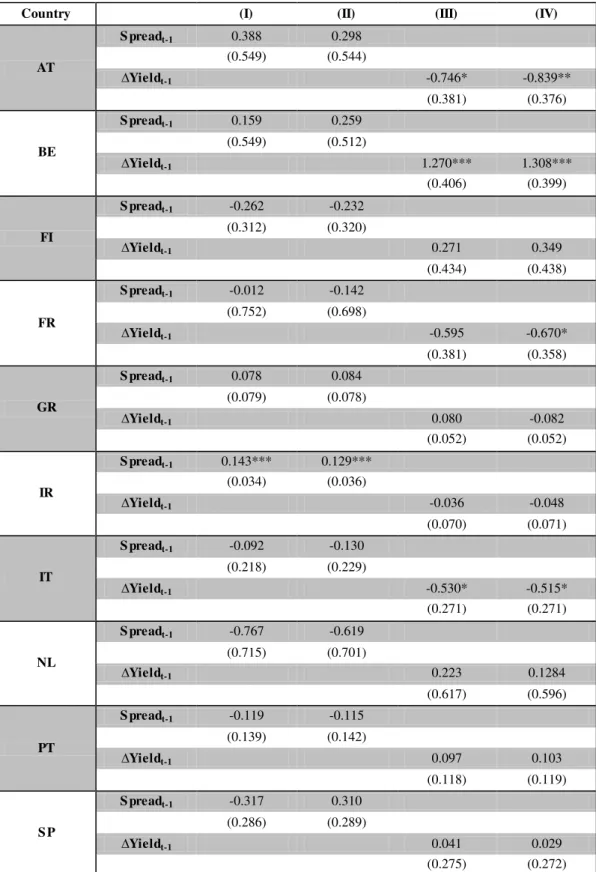
We now present the results concerning the spillover effects for the years t-1 and t in Table III and IV, respectively.
16
observe that there is a possible contagion from the spreads of Ireland, affecting negatively the whole country sample by 0.136 p.p.. Looking at the change in yields, only Belgium has an upward contagion effect on the spreads, increasing the overall spreads by 1.289 p.p., on average. On the other hand, a positive variation in the yields of Austria, France and Italy decrease the sample spreads (0.793 p.p., 0.670 p.p. and 0,523 p.p., respectively).
Regarding estimation results for the contagion effects in a contemporaneous fashion (Table IV) analysing the regression model (1) and (2), the spreads of Ireland still have a significant impact, increasing spreads in 0.095 p.p. on average. On the other hand, the spreads of Italy reduce the sample spreads by 0.147 p.p.. In terms of specification including the variation of the yields, only the change of yield of Belgium still has an impact, affecting negatively the spreads by 0.283 p.p.
17
Table III - Estimation results for the spillover effects in t-1
Note: the asterisks *, ** and *** represent significance at 10, 5 and 1% level, respectively. The values between parentheses are the standard error.
Country (I) (II) (III) (IV)
AT
S preadt-1 0.388 0.298
(0.549) (0.544)
∆Yieldt-1 -0.746* -0.839**
(0.381) (0.376)
BE
S preadt-1 0.159 0.259
(0.549) (0.512)
∆Yieldt-1 1.270*** 1.308***
(0.406) (0.399)
FI
S preadt-1 -0.262 -0.232
(0.312) (0.320)
∆Yieldt-1 0.271 0.349
(0.434) (0.438)
FR
S preadt-1 -0.012 -0.142
(0.752) (0.698)
∆Yieldt-1 -0.595 -0.670*
(0.381) (0.358)
GR
S preadt-1 0.078 0.084
(0.079) (0.078)
∆Yieldt-1 0.080 -0.082
(0.052) (0.052)
IR
S preadt-1 0.143*** 0.129***
(0.034) (0.036)
∆Yieldt-1 -0.036 -0.048
(0.070) (0.071)
IT
S preadt-1 -0.092 -0.130
(0.218) (0.229)
∆Yieldt-1 -0.530* -0.515*
(0.271) (0.271)
NL
S preadt-1 -0.767 -0.619
(0.715) (0.701)
∆Yieldt-1 0.223 0.1284
(0.617) (0.596)
PT
S preadt-1 -0.119 -0.115
(0.139) (0.142)
∆Yieldt-1 0.097 0.103
(0.118) (0.119)
S P
S preadt-1 -0.317 0.310
(0.286) (0.289)
∆Yieldt-1 0.041 0.029
18
Table IV - Estimation results for spillover effects, in t
Note: the asterisks *, ** and *** represent significance at 10, 5 and 1% level, respectively. The values between parentheses are the standard error.
Country (1) (2) (3) (4)
AT
S preadt 0.108 0.089
(0.113) (0.111)
∆Yieldt -0.186 -0.175
(0.124) (0.124)
BE
S preadt 0.095 0.102
(0.104) (0.105)
∆Yieldt 0.285* 0.280*
(0.161) (0.162)
FI
S preadt -0.091 -0.081
(0.149) (0.143)
∆Yieldt -0.149 -0.162
(0.104) (0.104)
FR
S preadt 0.004 -0.005
(0.146) (0.147)
∆Yieldt -0.122 -0.112
(0.119) (0.117)
GR
S preadt -0.021 -0.020
(0.026) (0.026)
∆Yieldt 0.024 0.021
(0.034) (0.034)
IR
S preadt 0.095*** 0.094***
(0.029) (0.028)
∆Yieldt 0.005 0.002
(0.064) (0.063)
IT
S preadt -0.146** -0.147**
(0.061) (0.060)
∆Yieldt 0.045 0.059
(0.155) (0.155)
NL
S preadt 0.262 0.238
(0.221) (0.220)
∆Yieldt -0.053 -0.071
(0.131) (0.123)
PT
S preadt 0.037 0.037
(0.039) (0.037)
∆Yieldt 0.050 0.053
(0.095) (0.093)
S P
S preadt -0.071 -0.068
(0.066) (0.067)
∆Yieldt 0.208 0.197
19
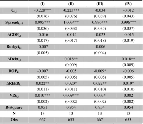
4.2. Robustness
In order to check the robustness of the results, we extend our sample to three more countries outside Euro Area, Denmark, Sweden and the United Kingdom, to test if the spillover effects can spread to the non-Euro area countries for this particular assessment, we have not used the variable bid-ask spread due to the fact that it is not available for these countries. We based our analysis in the same models described before.
In Table V, we report the results of the estimation for the spreads of 10-years government bond yields: columns (I) and (II) report estimation for model (1), and columns (III) and (IV) for the model (2).
20
Table V - Estimation results for the determinants of 10-years yield spreads: models (1) and (2)
(I) (II) (III) (IV)
Ci,t -0.228*** -0.223*** -0.034 -0.012
(0.076) (0.076) (0.039) (0.043)
S preadi,t-1 0.995*** 1.003*** 0.996*** 0.996***
(0.036) (0.038) (0.035) (0.037)
∆GDPi,t -0.016 -0.014 -0.023 -0.015
(0.017) (0.017) (0.018) (0.019)
Budgeti,t -0.007 -0.006
(0.005) (0.004)
∆Debti,t 0.018** 0.018**
(0.009) (0.009)
BOPi,t -0.007 -0.005 -0.009* -0.006
(0.005) (0.005) (0.005) (0.005)
∆REERi,t 0.022** 0.020* 0.022** 0.019*
(0.011) (0.011) (0.010) (0.010)
VIXi,t 0.010*** 0.009*** 0.003* 0.002
(0.002) (0.002) (0.002) (0.002)
R-S quare 0.951 0.954 0.954 0.954
N 13 13 13 13
Obs 667 653 667 653
Note: the asterisks *, ** and *** represent significance at 10, 5 and 1% level, respectively. The values between parentheses are the standard errors. N is the
number of countries included in the sample and Obs is the number of observations.
Table VI presents results for the models including the potential contagion spreads and the variations of the yields at period t: columns (I) and (II) refer to model (3), and columns (III) and (IV) to model (4).
21
Table VI - Estimation results for the determinants of 10-years yield spreads: models (3) and (4)
(I) (II) (III) (IV)
Ci,t -0.261*** -0.236*** -0.014 0.003
(0.067) (0.074) (0.044) (0.050)
S preadi,t-1 1.003*** 1.014*** 0.995*** 0.997***
(0.036) (0.037) (0.033) (0.033)
∆GDPi,t 0.006 0.005 -0.006 -0.003
(0.016) (0.017) (0.017) (0.018)
Budgeti,t -0.005 -0.006
(0.005) (0.005)
∆Debti,t 0.013 0.018**
(0.010) (0.008)
BOPi,t -0.007 -0.005 -0.007 -0.004
(0.006) (0.006) (0.005) (0.005)
∆REERi,t 0.022** 0.022** 0.012 0.010
(0.011) (0.010) (0.010) (0.010)
VIXi,t 0.007*** 0.006** 0.001 0.000
(0.002) (0.002) (0.002) (0.002)
R-S quare 9.948 0.950 0.951 0.953
N 13 13 13 13
Obs 667 653 667 653 Note: the asterisks *, ** and *** represent significance at 10, 5 and 1% level, respectively. The values present between parentheses are standard error. N is the number of countries included in the sample and Obs is the number of observation.
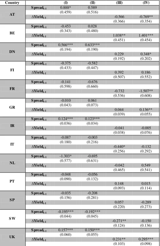
Focussing now our analysis on the spillover or contagion in period t-1, we can observe (see appendix B1) that in addition to the spreads of Ireland, the spreads of Denmark and of the United Kingdom have a significant impact on the spreads in the country sample, increasing spreads in 0.600, 0.124 and 0.154 p.p., respectively for Danish, Irish and British spreads, all on average. On the other hand, the spreads of the Netherlands and Sweden decrease in 1.303 and 0.193 p.p. the whole sample spread, respectively. Looking at the columns (III) and (IV), the positive variation of the yields of Belgium, Denmark, Greece and United Kingdom, inducing an increase spreads in 1.220, 0.348, 0.136 and 0.263 p.p. on average, respectively. The variation of the yields of Austria, France and Sweden decrease in 0.769, 1.507 and 0.271 p.p., respectively.
22
spreads in 0.210, 0.264, 0.062 and 0.191 p.p., respectively, on average. Regarding the Swedish spreads, they reduce the whole sample spread in 0.105 p.p., on average. Looking to the remaining columns, (III) and (IV), the positive variation of Belgian and Swedish yields, induce an increase in 0.501 p.p. and 0.245 p.p, respectively, on average. On the other hand, the variation of the yields of Denmark and United Kingdom decrease the whole sample spread in 0.163 and 0.208 p.p., respectively, both on average.
The analysis of the core variables seems to confirm the idea that the spreads depend significantly on the previous information. The disbelief in the capacity of a country to overcome the crisis led investors starting to give more importance to public debt. In addition, the real effective exchange rate shows have a great importance as indicator of the country's economic situation.
Regarding the impact of the spread and the variation of the yields of each country, the spread of Ireland and the variation of the yields of Belgium have an important effect in the whole EMU, as well as in the EU. Furthermore, the countries outside the Euro Area have a significant impact on the spreads, reflecting how the economic situation of the all European Union is important to stabilize the Euro Area.
4.3. Country estimation – SUR
23
Thus, some countries present higher fiscal imbalances and higher public debt, affecting their credibility and becoming more vulnerable to the feeble economic environment. Specifically, it is more likely that the peripheral countries, as Greece, Portugal and Ireland, are more affected by the sovereign debt crisis and exhibit a spillover effect than the core countries, as Austria, Finland and the Netherlands.
We have estimated a system of equations, one for each country, to find the individual coefficients. For this purpose, we employed the Seemingly Unrelated Regressions (SUR) model, which supposes that dependent variable and regressors may differ between equations, but contemporary correlation exists between residuals of all equations.
For our analysis, we will use a SUR model and estimate four specifications. Due to the lower significance of the budget balance, we have excluded this variable from our analysis and only included the public debt ratio. The model is as follows:
(5) = β0 + β1* + β2.* i,t+ β3*vixt+ β4*bidi,t + j,t*
(6) = α0 + α1* + α2.* i,t+ α3*vixt+ α4*bidi,t + i,t*
(7) = β0 + β1* + β2.* i,t+ β3*vixt+ β4*bidi,t + j,t*
(8) = α0 + α1* + α2.* i,t+ α3*vixt+ α4*bidi,t + j,t*
From the four equations above, we create a system of ten regressions, one for each country (Austria, Belgium, Finland, France, Greece, Ireland, Italy, Netherlands, Portugal and Spain).
24
tables D1, D2, D3 and D4, we also present the results using the budget balance.
Looking at the results, we observe that the coefficients and the significant variables obviously change across countries. In addition, while in the initial results, only the spread of Ireland and the variation of the yields of Belgium have an important impact, now the spreads and the variation of the yields of all countries have a significant effect on the various countries, reflecting the spillover effect. We briefly analyze below the results for each country.
Starting with Austria, the spread is positively correlated with the Belgian and Italian spreads and negatively with the spreads of France and Spain, at time t-1. Looking to the influence of the spreads in period t, the spreads of Belgium, Finland, France and Greece increase the Austrian spread, unlike the spread of Portugal and Spain which they have the opposite effect. Analyzing the impact of the variation of the yields in t-1, the spread of Austria is negatively correlated with the variation of the yields of France and positively with the variation yields of Portugal. At the period t, the Belgian and Greek variation of the yields increase the spread of Austria and the variation of the yields of Ireland and Italy decrease the Austrian spread.
25
spreads, unlike the variation yields of Finland, Greece and the Netherlands downward the Belgian spread.
For Finland, the spread in t-1 is positively correlated with the spreads of Austria, Belgium and Netherlands, and negatively correlated with the French and Spanish spreads. At time t, there are more countries influencing the Finnish spreads. In addition to the spreads of Austria, Belgium and Netherlands, the spreads of Portugal and Spain also increase Finnish spreads. On the other hand, the spreads of France, Greece, Ireland and Italy decrease the spread of Finland. For the results of the influence of the variation of the yields, the spread of Finland decreases when the variation of the yields of France and Ireland increase 1 p.p., as opposed to the variation of the yields of Portugal, the Finland's spread increase, at t-1. In the period t, the variation of the yields of Greece, Ireland, Italy and the Netherlands downward the Finnish spread and the Portugal and Spain's variation of the yields push up the Finnish spread.
In France, the spread in t-1 is affected negatively by the Portuguese spread (French spreads increase 0.151 p.p.) and positively by the spreads of France itself and Ireland. Regarding to the period t, the spreads of Austria, Belgium, the Netherlands, Portugal and Spain increase the French spread. The Finnish and Irish spread decrease the French spread. For the impact of the variation of the yields in t-1, Portugal push up the French spreads in 0.238 p.p., unlike France, Greece and Ireland. At time t, the variation of the yields of Austria, Finland, Ireland and Italy decrease the spread of France. On the other hand, the Belgium and Greece's variation of the yields are positively correlated with the French spread.
26
the Greek spread. Concerning the period t, in addition to the spreads of Italy and Spain, Austria and Portugal increase the Greek spread, and the Belgian and Dutch spreads are negatively correlated with the Greece's spread. For the variation of the yields in t-1, Austria, France, Greece and Portugal decrease spread. A positive variation of the Italian and Spanish yields increase the Greek spread. Looking to the period t, the variation of the yields of Belgium, Ireland and Netherlands are negatively correlated with the spread of Greece, unlike the variation of the yields of Italy and Portugal.
Ireland's spreads increase when the spreads in t-1 of Austria, Greece and Ireland itself increase and decrease when the spreads in t-1 of Netherlands, Portugal and Spain increase. In the period t, all spreads of the other countries have an impact on Irish Spreads. The spreads of Belgium, Greece, Netherlands and Spain increase the Irish spread, in contrast to the spreads of Austria, Finland, France, Italy and Portugal which they decrease Ireland's spread. Concerning the variation of the yields in t-1, a positive variation of the yields of Greece and Ireland itself increase the spreads, unlike Portugal and Spain. Looking to the period t, the variation of the yields of Austria, Finland, France and Italy are negatively correlated with Irish spreads. On the other hand, the variation of the yields of Belgium, Netherlands, Portugal and Spain increase the spreads of Ireland.
For Italy, in t-1, the spreads of Ireland, Netherlands and Portugal increase the Italian spread, unlike the spread of Finland. For the period t, the spreads of Belgium, Netherlands and Spain are positively correlated with the Italian spread. On the other hand, an increase in the spreads of Austria, Finland, Greece and Ireland decrease the spread of Italy. Regarding the results of the influence of the variation of the yields in
27
with the Italian spread, as opposed to the Austrian, Finnish and Irish variation yields. The variation of the yields in t of Belgium and Portugal increase Italian spread. The variation of the yields of Austria, France and Ireland in t downward the Italy's spread.
Looking to the results for the Netherlands, the spillover effect of the spreads of each country has more impact than the influence of the variation yields. Concerning the period t-1, except for the Belgium spreads, all spreads have an impact on the Dutch spread. The spreads of Finland, France, Portugal and Spain decrease the spread of the Netherlands, as opposed to the remaining countries. At time t, in addition to the spreads of Portugal and Spain pushing down the Dutch spreads, now the spread of Belgium is significant in the same way. The spreads in t of France, Finland, Ireland and Italy are positively correlated. The variation of the yields of Greece and France in t-1 decrease and increase the spread of Netherlands, respectively. The Belgian and Finnish variation yields in t are negatively correlated with the Dutch spread, on the other hand, a positive variation in the yields of France and Spain induce an increase in the spread of the Netherlands.
28
The Belgian and Greek variation of the yields in t increase Portuguese spread, unlike the variation of the yields of France and Spain.
Finally, analyzing the results for Spain, an increase in spreads, in t-1, of Austria, France, Greece and Ireland induce an increase in Spanish spreads, on the other hand, an increase in Italian and Dutch spreads have the opposite effect. For the period t, the spreads of Belgium, Finland, Greece, Italy and Netherlands increase the spread of Spain and the spreads of Austria and Portugal are negatively correlated with the Spanish spread. Regarding the variation of the yields of France and Greece in t-1, when they increase 1 p.p., the Spanish spreads also increases, in contrast when there is a positive variation in the Italian yields, the spread of Spain decreases. At time t, the variation of the yields of Belgium, France, Greece, Ireland and Italy are positively correlated with the Spanish spread, as opposed to the Austrian and Portuguese variation of the yields.
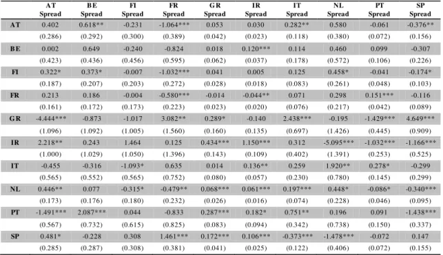
As expected, the spillover effect from Greece, Ireland and Portugal tend to be higher than in other countries. In addition, Belgium, Italy, Netherlands and Spain also have a great influence in the spreads of the other countries, due to the deterioration in their fiscal and macroeconomic fundamentals, namely higher public debt. On the other hand, Austria, Finland and France are affected too, but they have a positive impact in almost all countries and still maintain the credibility in their economies. After making the individual analysis, it is evident to the presence of contagion between the EMU countries.
29
spreads of the other countries, supporting the idea that the stability of the EMU countries is affected by the countries outside the Euro area.
Table VII - Spillover effect for model (5)
AT Spread
B E Spread
FI Spread
FR Spread
G R Spread
IR Spread
IT Spread
NL Spread
PT Spread
SP Spread
AT 0.402 0.618** -0.231 -1.064*** 0.053 0.030 0.282** 0.580 -0.061 -0.376**
(0.286) (0.292) (0.300) (0.389) (0.042) (0.023) (0.118) (0.380) (0.072) (0.156)
B E 0.002 0.649 -0.240 -0.824 0.018 0.120*** 0.114 0.460 0.099 -0.307
(0.423) (0.436) (0.456) (0.595) (0.062) (0.037) (0.178) (0.572) (0.106) (0.226)
FI 0.322* 0.373* -0.007 -1.032*** 0.041 0.005 0.125 0.458* -0.041 -0.174*
(0.187) (0.207) (0.203) (0.272) (0.028) (0.018) (0.083) (0.261) (0.048) (0.103)
FR 0.213 0.186 -0.004 -0.580*** -0.014 -0.044** 0.071 0.298 0.151*** -0.116
(0.161) (0.172) (0.173) (0.223) (0.023) (0.020) (0.076) (0.217) (0.042) (0.089)
G R -4.444*** -0.873 -1.017 3.082** 0.289* -0.140 2.438*** -0.195 -1.429*** 4.649***
(1.096) (1.092) (1.005) (1.560) (0.160) (0.135) (0.697) (1.426) (0.445) (0.909)
IR 2.218** 0.243 1.464 0.125 0.434*** 1.150*** 0.312 -5.095*** -1.032*** -1.166***
(1.000) (1.029) (1.050) (1.396) (0.143) (0.109) (0.402) (1.391) (0.253) (0.525)
IT -0.455 -0.316 -1.093* 0.635 0.014 0.136** 0.259 1.920** 0.278* -0.299
(0.565) (0.552) (0.565) (0.752) (0.080) (0.057) (0.230) (0.780) (0.145) (0.299)
NL 0.446** 0.077 -0.315* -0.479** 0.068*** 0.061*** 0.197*** 0.448* -0.086* -0.340***
(0.173) (0.176) (0.180) (0.232) (0.026) (0.016) (0.074) (0.228) (0.046) (0.095)
PT -1.491*** 2.087*** 0.044 -0.833 0.287*** 0.182* 0.751** 0.196 0.091 -1.438***
(0.567) (0.732) (0.615) (0.825) (0.083) (0.094) (0.342) (0.738) (0.150) (0.337)
SP 0.481* -0.228 0.308 1.461*** 0.172*** 0.106*** -0.373*** -1.478*** -0.072 0.147
(0.285) (0.287) (0.308) (0.381) (0.041) (0.025) (0.122) (0.406) (0.072) (0.155)
30
Table VIII – Spillover effects model (6)
AT
∆Yield ∆YieldB E ∆YieldFI ∆YieldFR ∆YieldG R ∆YieldIR ∆YieldIT ∆YieldNL ∆YieldPT ∆YieldSP
AT 0.055 0.252 0.042 -0.496* 0.005 -0.056 0.080 0.022 0.121*** -0.026
(0.208) (0.265) (0.224) (0.263) (0.023) (0.037) (0.118) (0.295) (0.042) (0.114)
B E -0.265 -0.328 -0.202 -0.116 -0.004 0.032 0.195 0.262 0.341*** 0.083
(0.314) (0.402) (0.352) (0.393) (0.036) (0.059) (0.190) (0.441) (0.068) (0.183)
FI 0.089 0.322 -0.019 -0.641*** 0.009 -0.074** -0.072 0.333 0.069* 0.073
(0.171) (0.231) (0.195) (0.223) (0.019) (0.034) (0.108) (0.258) (0.037) (0.101)
FR 0.174 -0.010 0.026 -0.326* -0.036** -0.108*** -0.063 -0.048 0.238*** 0.131
(0.155) (0.201) (0.172) (0.194) (0.018) (0.026) (0.089) (0.215) (0.033) (0.088)
G R -3.393*** 0.500 0.068 -2.415** -0.210* 0.272 3.056*** 0.467 -1.445** 3.133***
(0.771) (0.783) (0.812) (1.087) (0.117) (0.212) (0.566) (1.171) (0.583) (0.838)
IR 0.441 0.096 0.318 0.922 0.262*** 1.006*** 0.579 -0.759 -0.625*** -2.078***
(0.749) (0.970) (0.914) (0.983) (0.089) (0.139) (0.447) (1.128) (0.191) (0.484)
IT -1.073* 0.205 -1.647*** -0.202 0.015 -0.194* -0.425 1.725** 0.670*** 0.948***
(0.567) (0.739) (0.613) (0.699) (0.065) (0.096) (0.336) (0.811) (0.122) (0.337)
NL 0.161 0.264 -0.096 -0.362* 0.037* -0.045 -0.153 0.174 0.024 0.028
(0.161) (0.212) (0.182) (0.203) (0.019) (0.029) (0.098) (0.229) (0.035) (0.092)
PT -1.083** 1.639*** 0.189 -0.857* 0.310*** 0.172** 0.849*** 1.249** -0.536*** -1.812***
(0.426) (0.579) (0.487) (0.519) (0.048) (0.070) (0.245) (0.600) (0.097) (0.253)
SP -0.271 -0.015 -0.353 0.708* 0.240*** 0.029 -0.371* 0.134 -0.115 0.119
(0.342) (0.446) (0.411) (0.423) (0.040) (0.065) (0.200) (0.510) (0.091) (0.234)
Note: the asterisks *, ** and *** represent significance at 10, 5 and 1% level, respectively. The values between parentheses are the standard error.
Table IX- Spillover effects from model (7):
AT Spread B E Spread FI Spread FR Spread G R Spread IR Spread IT Spread NL Spread PT Spread SP Spread
AT - 0.446*** 0.508*** 0.301** 0.024*** -0.012 -0.047 0.077 -0.060*** -0.067***
(0.073) (0.124) (0.129) (0.009) (0.011) (0.044) (0.137) (0.017) (0.034)
B E 0.725*** - 0.203 0.542*** -0.012 0.097*** 0.309*** -0.949*** 0.045* -0.157***
(0.144) (0.185) (0.181) (0.012) (0.013) (0.061) (0.173) (0.023) (0.053)
FI 0.346*** 0.165* - -0.316** -0.034*** -0.053*** -0.177*** 0.726*** 0.083*** 0.163***
(0.099) (0.085) (0.129) (0.007) (0.012) (0.042) (0.105) (0.016) (0.032)
FR 0.200* 0.389*** -0.251** - 0.001 -0.077*** -0.054 0.418*** 0.036*** 0.048*
(0.103) (0.077) (0.107) (0.007) (0.010) (0.039) (0.093) (0.014) (0.028)
G R 3.424*** -4.314*** -1.081 1.156 - -0.121 0.843* -4.429*** 1.347*** 3.272***
(0.851) (1.106) (0.798) (1.536) (0.146) (0.475) (1.311) (0.367) (0.770)
IR -1.623** 3.401*** -1.679** -2.273*** 0.166*** - -1.952*** 6.185*** -0.194* 0.652***
(0.665) (0.391) (0.749) (0.726) (0.051) (0.219) (0.651) (0.113) (0.208)
IT -1.211*** 1.504*** -1.192*** 0.064 -0.038* -0.165*** - 2.508*** 0.081 0.425***
(0.383) (0.277) (0.337) (0.338) (0.022) (0.026) (0.340) (0.050) (0.081)
NL 0.000 -0.332*** 0.700*** 0.420*** 0.013 0.067*** 0.178*** - -0.057*** -0.111***
(0.136) (0.095) (0.123) (0.137) (0.009) (0.012) (0.054) (0.018) (0.038)
PT -0.973*** 3.073*** 1.061*** -3.373*** 0.200*** -0.257*** -0.640*** 1.489*** - -0.614***
(0.326) (0.479) (0.407) (0.648) (0.020) (0.069) (0.220) (0.440) (0.096)
SP -2.144*** 0.983*** 0.935*** 0.193 0.191*** 0.041 0.290** 1.153*** -0.359*** -
(0.281) (0.286) (0.323) (0.322) (0.016) (0.028) (0.143) (0.394) (0.035)
31
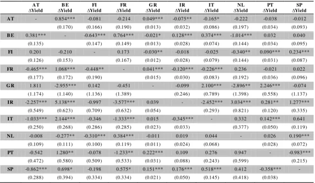
Table X – Spillover effects for model (8)
AT
∆Yield ∆YieldB E ∆YieldFI ∆YieldFR ∆YieldG R ∆YieldIR ∆YieldIT ∆YieldNL ∆YieldPT ∆YieldSP
AT - 0.854*** -0.081 -0.214 0.049*** -0.075** -0.165* -0.222 -0.038 -0.012
(0.170) (0.166) (0.190) (0.013) (0.032) (0.086) (0.197) (0.034) (0.093)
B E 0.381*** - -0.643*** 0.764*** -0.021* 0.128*** 0.374*** -1.014*** 0.032 0.040
(0.135) (0.147) (0.149) (0.013) (0.028) (0.074) (0.144) (0.034) (0.095)
FI 0.201 -0.210 - 0.173 -0.030** -0.018 -0.025 -0.340** 0.090*** 0.234***
(0.126) (0.153) (0.167) (0.012) (0.028) (0.079) (0.144) (0.031) (0.087)
FR -0.465*** 1.068*** -0.448** - 0.041*** -0.120*** -0.226*** 0.236 -0.021 0.022
(0.177) (0.172) (0.190) (0.015) (0.030) (0.083) (0.192) (0.036) (0.096)
G R 1.811 -2.955*** 0.142 -0.451 - -0.099 2.100*** -2.896** 2.246*** -0.074
(1.174) (1.140) (1.136) (1.389) (0.246) (0.789) (1.398) (0.558) (1.137)
IR -2.257*** 5.138*** -0.997 -3.577*** 0.039 - -2.452*** 3.034*** 0.281** 1.277***
(0.549) (0.623) (0.709) (0.632) (0.054) (0.293) (0.821) (0.120) (0.335)
IT -1.033*** 2.144*** -0.346 -1.333*** 0.015 -0.345*** - 0.332 0.142*** 0.641
(0.250) (0.268) (0.286) (0.285) (0.023) (0.033) (0.377) (0.050) (0.119)
NL -0.008 -0.277** -0.310*** 0.384*** -0.011 0.019 0.044 - 0.026 0.190***
(0.109) (0.111) (0.100) (0.119) (0.011) (0.024) (0.068) (0.028) (0.072)
PT -0.542 1.280** -0.078 -1.233** 0.222*** 0.109 0.276 0.947 - -0.983***
(0.472) (0.580) (0.509) (0.533) (0.031) (0.088) (0.243) (0.599) (0.215)
SP -0.862*** 0.698* -0.198 0.575* 0.151*** 0.176*** 0.518*** 0.412 -0.358*** -
(0.288) (0.394) (0.334) (0.334) (0.021) (0.050) (0.145) (0.418) (0.038)
Note: the asterisks *, ** and *** represent significance at 10, 5 and 1% level, respectively. The values between parentheses are the standard error.
5. Conclusion:
We have studied the spillover effect of spreads and of the variation of 10-years government bond yields in the European Union. We employ a panel of thirteen countries (Austria, Belgium, Denmark, Finland, France, Greece, Ireland, Italy, Netherlands, Portugal, Spain, Sweden and United Kingdom) using quarterly data over the period 2000:Q1-2013:Q1. We investigate the role of an extended set of potential spreads' determinants, namely international risk, liquidity conditions and macroeconomic and fiscal fundamentals, and the risk of transmission among the EU countries.
32
33
References
Afonso, A., Arghyrou, M. and Kontonikas, A. (2012). “The determinants of sovereign bond yield spreads in the EMU”, Department of Economics, ISEG-UTL, Working
Paper 36/2012/DE/UECE.
Arghyrou, M. and Kontonikas, A. (2011). “The EMU sovereign-debt crisis: Fundamentals, expectations and contagion”, European Commission, Economic
Papers 436.
Barrios, S., Iversen, P., Lewandowska, M., and Setzer, R. (2009). “Determinants of
intra-euro-area government bond spreads during the financial crisis”, European
Commission, Economic Paper 388.
Bernoth, A. and Erdogan, B. (2010). “Sovereign bond yield spreads: A time-varying
coefficient approach”, Department of Business Administration and Economics,
European University Frankfurt (Oder), Discussion paper 289.
Bernoth, K., von Hagen, J., Schuknecht, L. (2004). “Sovereign risk premia in the European government bond market”. ECB Working Paper 369.
Caceres, C., Guzzo, V. and Segoviano, M. (2010). “Sovereign Spreads: Global Risk
Aversion, Contagion or Fundamentals?”, IMF Working Paper 10/120.
De Santis, R. (2012). “The Euro Area sovereign debt crisis – safe haven, credit rating
agencies and the spread of the fever from Greece, Ireland and Portugal”, ECB
Working Paper 1419.
Favero, C., Pagano, M., von Thadden, E.-L. (2010). “How Does Liquidity Affect
34
Gerlach, S., Schulz, A., Wolff, G. (2010). “Banking and Sovereign Risk in the Euro
Area”. CEPRF Discussion Paper No. 7833.
Geyer, A., Kossmeier, S., Pichler, S. (2003). “Measuring Systematic Risk in EMU
Government Yield Spreads”. Review of Finance, 8, 171-197.
Giordano, L., Linciano, N. and Soccorso, P. (2012). “The determinants of government yield spreads in the euro area”, Commissione Nazionale Per Le Società e La Borsa,
Working Paper 71.
Jankowitsch, R., Mösenbacher, H., Picheler, S. (2006). “Measuring the Liquidity Impact
on EMU government bond prices”. European Journal of Finance, 12, 153-169.
Kilponen, J., Laakkonen, H. and Vilmunen, J. (2012). “Sovereign risk, European crisis
resolution policies and bond yields”, Bank of Finland Research Discussion Papers
22.
Missio, S., and Watzja, S. (2011). “Financial Contagion and the European Debt Crisi”.
Ludwig-Maximilian-University of Munich.
Pagano, M. and von Thadden, E.L. (2004). “The European bond market under EMU”,
Oxford Review of Economic Policy, 20, 531-554.
Pericoli, M. and Sbracia, M (2011). “A Primer on Financial Contagion”. Temi di
discussion del Servizio Studi, Banca d’Italia, Working Paper 407.
Schuknecht, L., von Hagen, J., Wolswijk, G. (2010). “Government bond risk premiums
in the EU revisited: The impact of the financial crisis”. ECB Working Paper 1152.
Sgherri, S. and Zoli, E. (2009). “Euro area sovereign risk during the crisis”, IMF
35
Appendix A – Core variables:
Table A1 - Random effects analysis for 10 countries
t-1 t-1 t t
Ci,t -0.096** -0.083* -0.096** -0.083*
(0.047) (0.049) (0.047) (0.049)
S preadi,t-1 0.822*** 0.818*** 0.822*** 0.818***
(0.046) (0.045) (0.046) (0.045)
∆GDPi,t -0.011 -0.007 -0.012 -0.007
(0.019) (0.019) (0.019) (0.019)
Budgeti,t -0.003 -0.003
(0.003) (0.003)
∆Debti,t 0.016** 0.016**
(0.007) (0.007)
BOPi,t -0.010*** -0.010*** -0.010*** -0.010***
(0.002) (0.002) (0.003) (0.002)
∆REERi,t 9.117** 8.497** 0.090** 0.084**
(3.664) (3.673) (0.037) (0.037)
VIXi,t 0.004** 0.004** 0.004** 0.004**
(0.002) (0.002) (0.002) (0.002)
BIDi,t 0.007*** 0.007*** 0.007*** 0.007***
(0.001) (0.001) (0.001) (0.001)
R-S quare 0.958 0.958 0.958 0.958
N 10 10 10 10
Obs 503 500 503 500
36
Appendix B – Spillover effects for the EU countries:
Table B1 - Spillover effects in t-1 for 13 countries
Note: the asterisks *, ** and *** represent significance at 10, 5 and 1% level, respectively.
Country (I) (II) (III) (IV)
AT
S preadt-1 0.888* 0.589
(0.459) (0.516)
∆Yieldt-1 -0.566 -0.769**
(0.366) (0.354)
BE
S preadt-1 -0.453 0.028
(0.343) (0.480)
∆Yieldt-1 1.038** 1.401***
(0.451) (0.454)
DN
S preadt-1 0.566*** 0.633***
(0.194) (0.190)
∆Yieldt-1 0.229 0.348*
(0.192) (0.202)
FI
S preadt-1 -0.375 -0.582
(0.433) (0.447)
∆Yieldt-1 0.392 0.186
(0.507) (0.552)
FR
S preadt-1 -0.141 -0.676
(0.598) (0.660)
∆Yieldt-1 -0.732 -1.507**
(0.536) (0.608)
GR
S preadt-1 -0.010 0.061
(0.043) (0.073)
∆Yieldt-1 0.044 0.136**
(0.039) (0.055)
IR
S preadt-1 0.124*** 0.123***
(0.036) (0.034)
∆Yieldt-1 -0.041 -0.005
(0.038) (0.076)
IT
S preadt-1 -0.087 -0.003
(0.180) (0.216)
∆Yieldt-1 -0.440* -0.132
(0.256) (0.292)
NL
S preadt-1 -1.303* -0.695
(0.577) (0.631)
∆Yieldt-1 -0.042 0.549
(0.465) (0.541)
PT
S preadt-1 -0.048 -0.056
(0.090) (0.132)
∆Yieldt-1 0.148 0.015
(0.093) (0.114)
S P
S preadt-1 -0.035 -0.208
(0.156) (0.281)
∆Yieldt-1 0.057 -0.289
(0.220) (0.273)
S W
S preadt-1 -0.195*** -0.192***
(0.044) (0.045)
∆Yieldt-1 -0.271** -0.150
(0.124) (0.136)
UK
S preadt-1 0.157*** 0.150***
(0.060) (0.055)
∆Yieldt-1 0.231** 0.295***
37
Table B2 - Spillover effects in t for 13 countries
Note: the asterisks *, ** and *** represent significance at 10, 5 and 1% level, respectively.
Country (I) (II) (III) (IV)
AT
S preadt -0.106 -0.122
(0.117) (0.111)
∆Yieldt -0.074 -0.064
(0.114) (0.112)
BE
S preadt 0.212* 0.208*
(0.114) (0.115)
∆Yieldt 0.506*** 0.495***
(0.172) (0.174)
DN
S preadt 0.195 0.264*
(0.152) (0.144)
∆Yieldt -0.172 -0.163*
(0.105) (0.097)
FI
S preadt 0.015 -0.003
(0.143) (0.141)
∆Yieldt 0.038 0.018
(0.101) (0.090)
FR
S preadt -0.015 -0.028
(0.132) (0.132)
∆Yieldt 0.117 0.110
(0.131) (0.131)
GR
S preadt -0.006 -0.006
(0.027) (0.028)
∆Yieldt 0.053 0.045
(0.036) (0.036)
IR
S preadt 0.062 0.062**
(0.027) (0.027)
∆Yieldt 0.038 0.028
(0.064) (0.063)
IT
S preadt -0.062 -0.058
(0.063) (0.067)
∆Yieldt -0.032 -0.048
(0.152) (0.158)
NL
S preadt -0.067 -0.065
(0.200) (0.197)
∆Yieldt 0.019 -0.018
(0.130) (0.123)
PT
S preadt 0.001 0.002
(0.048) (0.048)
∆Yieldt -0.088 -0.053
(0.095) (0.095)
S P
S preadt -0.034 -0.037
(0.057) (0.063)
∆Yieldt 0.041 0.072
(0.182) (0.190)
S W
S preadt -0.107** -0.102**
(0.048) (0.050)
∆Yieldt -0.255*** -0.234***
(0.084) (0.081)
UK
S preadt 0.196*** 0.185***
(0.047) (0.050)
∆Yieldt -0.204*** -0.211***