M
ASTER OF
S
CIENCE IN
FINANCE
M
ASTER
´
S
F
INAL
W
ORK
DISSERTATION
CAN
MODEL-BASED
FORECASTS
PREDICT
STOCK
MARKET
VOLATILITY
USING
RANGE-BASED
AND
IMPLIED
VOLATILITY
AS
PROXIES?
RICHARD
FOLGER
ZHAO
M
ASTER OF
S
CIENCE IN
FINANCE
M
ASTER
´
S
F
INAL
W
ORK
DISSERTATION
CAN
MODEL-BASED
FORECASTS
PREDICT
STOCK
MARKET
VOLATILITY
USING
RANGE-BASED
AND
IMPLIED
VOLATILITY
AS
PROXIES?
RICHARD
FOLGER
ZHAO
S
UPERVISION:
NUNO
SOBREIRA
Abstract
This thesis attempts to evaluate the performance of parametric time series models and RiskMetrics methodology to predict volatility. Range-based price estimators and Model-free implied volatility are used as a proxy for actual ex-post volatility, with data collected from ten prominent global volatility indices. To better understand how volatility behaves, different models from the Generalized Autoregressive Conditional Heteroskedasticity (GARCH) class were selected with Normal, Student-t and Generalized Error distribution (GED) innovations. A fixed rolling window methodology was used to estimate the models and predict the movements of volatility and, subsequently, their forecasting performances were evaluated using loss functions and regression analysis.
The findings are not clear-cut; there does not seem to be a single best performing GARCH model. Depending on the indices chosen, for range-based estimator, APARCH (1,1) model with normal distribution overall outperforms the other models with the noticeable exception of HSI and KOSPI, where RiskMetrics seems to take the lead. When it comes to implied volatility prediction, GARCH (1,1) with Student-t performs relative well with the exception of UKX and SMI indices where GARCH (1,1) with Normal innovations and GED seem to do well respectively. Moreover, we also find evidence that all volatility forecasts are somewhat biased but they bear information about the future volatility.
Keywords: Implied Volatility, Range-based Volatility, GARCH, Forecasting Accuracy,
Information Content.
Acknowledgement
I would like to thank my supervisor Nuno Sobreira for his support, guidance and prompt responses and suggestions through the entire process. I would not be able to use statistical software Eviews at ease without his guidance.
I would also like to thank Professor Maria Teresa Medeiros Garcia for guiding me through the administrative process for this Master of Final Work.
Table of Contents
1. INTRODUCTION ... 1
2. LITERATURE REVIEW ... 4
3. THEORETICAL CONCEPTS OF VOLATILITY ... 11
3.1VARIOUS TYPES OF VOLATILITY ... 11
3.1.1HISTORICAL VOLATILITY ... 11
3.1.2 Realized Volatility ... 12
3.1.3 Range-based Estimator as a Proxy for Actual Volatility ... 12
3.1.4 Option Implied Volatility as a Proxy for Actual volatility ... 13
3.1.4.1 Black-Scholes' Implied Volatility ... 13
3.1.4.2 Model-Free Implied Volatility ... 15
3.2CHARACTERISTICS OF VOLATILITY ... 17
4. DATA AND METHODOLOGY ... 19
4.1DATA COLLECTION AND FORECASTING METHOD DESCRIPTION ... 19
4.2VOLATILITY FORECASTING MODELS ... 21
4.2.1 Generalized Autoregressive Conditional Heteroscedasticity - GARCH ... 21
4.2.2 IGARCH (1,1) as a proxy for RiskMetrics ... 23
4.2.3 GJR-GARCH/TGARCH ... 23 4.2.4 Exponential GARCH ... 24 4.2.5 APARCH ... 24 4.3STATISTICAL DISTRIBUTION ... 25 4.3.1 Normal/Gaussian Distribution ... 25 4.3.2 Student-t Distribution ... 26
4.3.3 Generalized Error Distribution ... 26
4.4FORECASTING EVALUATION ... 26
4.4.1 Root Mean Square Error ... 27
4.4.2 Mean Absolute Error ... 27
4.4.3 Mean Absolute Percentage Error ... 27
4.4.4 Theil Inequality Coefficient ... 28
4.4.5 Information Content Univariate Regression ... 28
5. EMPIRICAL RESULTS ... 29
5.1DESCRIPTIVE STATISTICS ... 29
5.2OUT-OF-SAMPLE FORECAST EVALUATION ... 30
5.3INFORMATION CONTENT REGRESSION RESULT ... 32
6 CONCLUSIONS AND FUTURE RESEARCH ... 33
BIBLIOGRAPHY ... 36
APPENDICES ... 41
LIST OF TABLES AND FIGURE
List of tables
TABLE I:LIST OF EQUITY INDICES ALONG WITH ITS VOLATILITY INDICES ... 20
TABLE II:FORECASTING PERFORMANCE SUMMARY ... 30
TABLE III:DESCRIPTIVE STATISTICS OF RANGE ESTIMATOR AND IMPLIED VOLATILITY ... 42
TABLE IV:FORECASTING PERFORMANCE OF GARCH-TYPE MODELS ON RANGE ESTIMATOR ... 44
TABLE V:FORECASTING PERFORMANCE OF GARCH-TYPE MODELS ON MODEL-FREE IMPLIED VOLATILITY ... 46
TABLE VI:UNIVARIATE REGRESSION OF MINCER-ZARNOWITZ TO TEST INFORMATION CONTENT OF MODEL ON RANGE-BASED ESTIMATOR ... 48
TABLE VII:UNIVARIATE REGRESSION OF MICER-ZARNOWITZ TO TEST INFORMATION CONTENT OF MODEL ON IMPLIED VOLATILITY ... 49
List of Figure FIGURE 1:GRAPH OF EQUITY INDEX LEVEL ALONG WITH ITS VOLATILITY INDEX LEVEL (1/3/2005 -12/30/2016) ... 41
1. Introduction
Volatility is one of the most studied topics in modern finance. The ability to correctly forecast future volatility has been the interests of anyone who is involved in the financial market. In Finance, volatility is defined as the fluctuation of asset prices from its mean over a specific period of time, which is commonly calculated as standard deviation of its logarithmic returns.
Although, volatility does not translate the full risk in the market, but it is a good representation of the significant portion of risk that can be quantified. Therefore forecasting volatility is crucial in investment decision-making, valuing derivative products, risk
management and portfolio hedging. For example, in the notorious Black-Scholes (1973) equation based on the option-pricing model, volatility of the underlying asset over the life of the option is a fundamental input in the determination of the fair value of the derivative products. However volatility cannot be directly observed, but rather needs to be estimated, which again highlights the importance of being able to accurately forecasting volatility of underlying asset.
As a result, it comes as no surprise that forecasting market volatility has received a great deal of attention in recent times both in academia and among financial practitioners. The aim of this thesis is to evaluate the forecasting accuracy of RiskMetrics and various GARCH-type models against future volatility of ten globally traded equity indices. In this paper, both range estimators based on daily price information and model-free implied volatility, which is said to be the market participant’s expected future volatility, are used as
proxies for the actual ex-post volatility in the markets. This paper also investigates the information content of the most accurate model forecasts from each index to see if they indeed contain some additional information about future volatility.
Despite the vast amount of literature on the subject of volatility forecasting, it is rather difficult to draw a unanimous conclusion due to differences in research design in terms of asset classes, countries, sample period, forecasting techniques, forecasting horizon and evaluation measures. This thesis attempts to get a clearer picture of the performance of time series models by incorporating 10 globally traded indices within a common
framework.
Many studies attempt to forecast future realized volatility using model-based
forecasts such as Generalized Autoregressive Conditional Heteroscedasticity (GARCH) and others attempt to model volatility by using option implied volatility forecasts. The results are somewhat mixed mainly due to difference in research methodology. Poon and Granger (2003) compiled a detailed literature review on this subject and concluded that overall implied volatility seems to contain more information about future volatility than the time series forecasts and it outperforms all other models. When it comes to time series forecasts, models that take into account volatility asymmetric response to negative and positive news tend to outperform others.
In the work of this thesis, a variety of GARCH-type models and RiskMetrics along with Normal, Student-t and Generalized Error Distribution (GED) innovations are fitted through a fixed rolling window methodology to capture the movement of range-based and model-free implied volatility of 10 international equity indices. Afterwards, each individual model’s out-of-sample predicting performance is evaluated based on a number of
forecasting accuracy metrics to see which model tends to outperform the others. As proxies for the actual volatility we use range-based Parkinson (1980) estimator, which is said to be 5 times more efficient than the squared returns (Garman & Klass, 1980). We also
considered the implied volatility based on the model-free variance swap concept, which improves on Black-Scholes implied volatility by addressing the constant volatility assumption and symmetric Gaussian return assumption (Siripoulos & Fassas, 2009).
Though the results are mixed, but conclusions can be made. In forecasting volatility using Parkinson (1980) range-based estimator as a proxy, asymmetric GARCH(1,1) model such as APARCH (1,1) with Normal distribution are able to better capture the dynamics of volatility with exception of HSI (China) and KOSPI (Korea) where RiskMetrics excel. This seems to be in line with the conclusion from Poon and Granger (2003) that time series models that allow asymmetric effects perform well overall. However, when it comes to forecast volatility using implied volatility as proxy, simple GARCH (1,1) with Student-t innovation seems to be the one with better performance overall.
The content of this thesis is structured as follows. Section 2 presents relevant literature review of the volatility forecasting using both model-based and model-free implied volatility approaches. Theoretical concepts of volatility are presented in section 3 and section 4 elaborates on the methodologies and data used to carry out this research. The main findings of this research along with analysis are presented in section 5. The main conclusions and future research suggestions are detailed in section 6.
2. Literature Review
There is a wide variety of literature on the topic of volatility forecasting; in which some are focused more on model-based forecasting while others attempt to evaluate the forecasting accuracy of several models with implied volatility.
Earlier studies attempted to capture the dynamics of volatility using the
autoregressive moving average model (ARMA) and Box-Jenkins ARMA yield relatively low forecasting accuracy due to many of the characteristics of volatility such as the
clustering effect, asymmetric response to shocks, and heteroscedastic nature of the residual terms. (Tsay, 2010) Later on, ARCH model of Engle (1982) was developed to capture clustering effects of volatility and its non-linear dynamics. ARCH model estimates
conditional variance as a function using a number of lags of its past squared residuals. One of the shortcomings of ARCH model is it might require many lags in the conditional variance equation to better capture the dynamics of volatility, and it also means many coefficients would have to be estimated. Bollerslev (1986) and Taylor (1986) independently came up with a generalized version of ARCH called GARCH model, which limits the number of estimated parameters and it is said to be more parsimonious than the ARCH model. (Brook, 2008) Subsequently, many variations of ARCH/GARCH models were developed to capture the other stylized facts of volatility such as asymmetric response to shocks.
Akgiray (1989), one of the earliest researches to test the predictability of GARCH model concludes that GARCH consistently outperforms historical volatility and
researches testing the predictability of the GARCH model against other time series and implied volatilities mostly in major stock indices and foreign exchange rates. Cumby, Figlewski and Hasbrouck (1993) introduced Exponential GARCH model and concluded that EGARCH outperforms historical volatility model despite the low 𝑅!. Figlewski (1997)
concludes that GARCH model’s adequate performance is mostly restricted to stock market data and only for short horizon forecasting. There are many other studies that give mixed conclusions. As the methodology used in conducting research varies, the results could also be different. There are many factors that can affect the outcome of the study; such as different loss functions used in the evaluation, different sampling methodology (fixed rolling window estimation or recursive expanding estimation), or even different sample period for different asset could lead to rather different conclusion.
In a model-based volatility comparative research, Brownlees et al. (2011) evaluate the forecast accuracy of the ARCH family models with different horizons and study how the predictability can be affected by factors such as estimation window length, different distribution assumptions and re-estimation frequency for the parameters. The authors include a wide range of asset classes including numerous domestic and international equity indices as well as exchange rates. The models that the authors include in the study are: GARCH (1,1), TARCH, EGARCH, NGARCH, and Asymmetric power ARCH. The loss functions are Quasi-likelihood (QL) and mean square error (MSE) but the authors focused on QL and argued that QL’s bias is independent of volatility level while MSE’s bias is proportional to the true variance squared. In addition to the daily dividend adjusted log return data on S&P 500 index from 1990 to 2008, the authors also use 10 exchange rates, 9 domestic indices and 9 international indices and the out-of-sample forecasting period spans
from 2001 to 2008 covering period of both low volatility and crisis. First, forecasting performance of S&P 500 is assessed against daily-realized volatility and squared returns over a range of horizon and subsequently, a direct comparison of forecasts from the GARCH models during the full sample period with only the crisis period of fall 2008 are conducted and the results of the out-of-sample QL losses are reported using TARCH (1,1). The results show that asymmetric models such as TARCH model performs relatively well across asset classes, methods and sample periods including period of distress. The authors conclude that use the longest date series available seem to enhance the model performance and weekly parameter re-estimation is ideal to combat the parameter drifting. Innovation distribution such as student–t does not yield any improvement in predictability of the model. For period of extreme high distress such as fall 2008, short horizon forecast such as 1 day ahead forecast is able to capture the dynamic of volatility; the problem lies with long horizon forecasts (multistep forecasts).
Using implied volatility as a forecast of market’s expectation of future volatility has also gain popularity. Implied volatility is derived from Black-Scholes’ (1973) option pricing formula using the backward induction as all the inputs in the formula can be either observed or computed with the exception of volatility. However, Black-Scholes’ implied volatility suffers from discrepancy of volatility smile; where implied volatilities computed from options on the same underlying with the same maturity but different exercise prices yield different results that violate the theory, which states volatility is assumed constant over the life of the option. Many researchers decide to use At-the-money option implied volatility due to its liquidity and large trading volume, which can correct some of the market microstructure concerns. Despite its shortcomings, many articles claim implied
volatility can better predict realized volatility than their time series counterparts.
(Lamoureux and Lastrapes, 1993; Vasilellis and Meade, 1996) Since then there are numerous studies on predictability of implied volatility index (original “VIX”, now titled VXO) from the Chicago board of Option Exchange (CBOE). Many studies such as Fleming et al. (1995) use the old CBOE’s “VIX” implied volatility index based on the options of S&P 100 to forecast true volatility of equity index. Most studies seem to confirm that implied volatility contains crucial information about the future volatility. Fleming et al (1995), in addition to confirming that implied volatility performs better when comparing to first order autoregressive volatility models and also discover the strong inverse and
asymmetric relationship between the VXO implied volatility and its S&P 100 market price. Blair et al (2001) report the highest explanatory power of VXO implied volatility to the S&P 100 index and reach the similar conclusion that implied volatility seems to perform better than the model-based counterparts. In addition to Blair et al. (2001), Lamoureux and Lastrapes (1993), Canina and Figlewski (1993), and Fleming et al. (1995) all find implied volatility biases in their forecast of realized volatility.
Despite of its promising results from U.S stock market indices, many international, smaller indices seem to have mixed results. Frennberg and Hanssan (1996) study the Swedish market and find that implied volatility in fact, cannot outperform even the simple autoregressive and random walk model. Australian market study of implied volatility conducted by Brace and Hodgson (1991) yields very inconsistent forecasting outcomes. While Doidge and Wei (1998) find combination of GARCH and implied volatility to be ideal in forecasting the Canadian Toronto index volatility.
Poon and Granger (2003) in a comprehensive volatility forecasting review
summarize 93 studies on the matter of volatility forecasting and conclude that overall with mixed results, implied volatility seems to outperform other volatility forecasters that includes historical volatility model, random walk, autoregressive, moving average and exponential weights as well as GARCH/ARCH family models. Moreover, the authors report that time series models that take account of asymmetric response in volatility seems to perform better compared to others, such as EGARCH and TGARCH model.
In a study conducted by Martens and Zein (2004) in which the authors incorporate high frequency intraday data and long memory models to forecast volatility of 3 different asset classes: equity, foreign exchange and commodities. Data sample from S&P 500, Yen/USD, and Sweet crude oil start from beginning of 1994, 1996 and June 1993
respectively span to the end of 2000 from various sources. Implied volatility is calculated using the weighted average of two nearest at-the-money calls and puts and weights are selected where the average exercise price matches the underlying future prices. Realized volatility is calculated using the sum of squared intraday return rather than the standard squared daily return to avoid possible noise. Autoregressive fractionally integrated moving average is used to estimate log-realized volatility in addition to the GARCH (1,1) and recursive expanding rolling estimation method is used with initial in sample period of 500 observations. The loss function of Heteroskedasticity consistent Root Mean Squared Error is computed to evaluate the forecasting performance of the models. Implied volatility outperforms GARCH models and in encompassing analysis, implied volatility also subsumes mostly all the information content. Interestingly, the authors find long memory
model able to compete with implied volatilities and in some cases even outperforms
implied volatilities. Both measures contain information that the other does not possess. In a more recent study, Ryu (2012) investigates the information content and forecasting accuracy of the implied volatility index of KOSPI (South Korea) against RiskMetrics, Black-Scholes’ implied volatility and GJR-GARCH models. He argues that since option market of KOSPI ranks highest in terms of trading volume and investor’s interest, therefore the implied volatility index extracted from option prices should contain predictive information about future volatility. The implied volatility index of KOSPI (VKOSPI) is computed using the model-free methodology based on the concept of fair value variance swap and does not rely on any option pricing models; its calculation resembles the new VIX index from the S&P 500 U.S equity index. The total sample size contains 2,057 daily observations and using fixed rolling analysis with forecasting horizon of 1, 5, 10, 21, and 63 trading days and finally the results are evaluated using the Mincer-Zarnowitz decomposition of Mean Square Error. Ryu (2012) concludes that implied volatility index (VKOSPI) contains meaningful information about future volatility of KOSPI and it outperforms all other forecasters in predicting realized volatility. Moreover, when the forecasting horizon is 5, 10, and 21 trading days, more than half of the changes in realized volatility can be explained by the VKOSPI index. In studying the relationship between the volatility index and its underlying equity return, the author confirms the asymmetric inverse relationship between the two, which is a well documented in the literature. (French et al., 1987; Schwert, 1989,1990; Fleming 1995)
Shaikh and Padhi (2014) attempt to study the forecasting performance of Indian volatility index along with RiskMetrics GARCH, and GJR-GARCH (1,1) using both
overlapping and non-overlapping sampling procedure with roughly of 6 years span of daily data with forecasting horizon of 1, 5, 10, 22, and 66 days. Indian VIX index uses the same model-free implied volatility methodology as many of the global volatility indices and realized volatility is computed based on the sum of the squared returns. The performance measure is based on the loss functions of RMSE, MAE and Theil’s U statistics. For non-overlapping samples with exception of 1- day and 66-day forecasts, implied volatility outperforms other models and following by RiskMetrics. GJR-GARCH (1,1) seems to dominate the overlapping sample methods. Implied volatility also contains more
information about the future volatility than the other forecasts, especially in the case of 10-day and 22-10-day horizon showing the highest adjusted 𝑅!. Interestingly, the authors
conclude that based on the univariate and encompassing regression, implied volatility dominates other forecasts and it is unbiased and efficient estimator of the market volatility.
In an international-focused, comparative study of implied, realized and GARCH volatility forecasts conducted by Kourtis et al. (2016), where the authors use 13 global indices from 10 countries with different forecasting horizon (1, 5, 22 days) and under different market conditions (before, during and after crisis of 2008) to study the forecasting performance and information content of model-free implied volatility, random walk, GJR-GARCH and Heterogeneous Autoregressive (HAR) model. Daily realized volatility is calculated using square root of sum of intraday returns collected at 5 min equally spaced intervals and the data spans for roughly 12 years from 2000 to October 2012. Out-of-sample evaluation is illustrated by using the loss functions of RMSE and QLIKE and the results show that for daily horizon forecasts, HAR performs better while for weekly horizon, MFIV adjusted for risk premium (C-MFIV) and HAR are comparable and finally
monthly forecasting horizon shows that C-MFIV has the lowest forecasting errors. Separate out-of-sample evaluation is conducted for pre-crisis, crisis and after crisis period and the results show that while all models deteriorate during the crisis period, HAR and MFIV-C are better models compared to the rest in daily and monthly horizon. The authors also find that HAR has the greatest explanatory power for daily horizon, while C-MIFV contains more information about future realized volatility for monthly horizon.
3. Theoretical Concepts of Volatility
As volatility cannot be directly observed in the market, but rather needs to be
estimated from market indicators, and as this is the main focus of this thesis, it is instructive to take a deeper dive into the concepts of volatility and its common features.
3.1 Various Types of Volatility
3.1.1 Historical Volatility
There are many ways of calculating volatility in the financial world. Volatility is a statistical measure of the variation of the return over time for a given security or equity index and is usually expressed as the standard deviation of the log returns. Volatility is used as a form of risk measurement and is calculated using the formula below, where 𝜎 is the sample standard deviation (volatility), 𝑟! is the return observed and 𝑟 is the mean return.
𝜎 = !!!! ! 𝑟!− 𝑟 !
In this thesis and as it is standard in the financial econometrics literature, the return 𝑟! is calculated under the continuous compounding framework as log difference of price P at time t and price at the previous period 𝑃!!!, which gives the following formula.
𝑟! = ln ( !!
!!!!) (2)
3.1.2 Realized Volatility
When evaluating the forecasting accuracy of various potential predictors it is crucial to select a good proxy for the true ex post volatility. One option is to use historical
volatility, which typically uses daily closing price, but a lot of intraday information could be lost using historical closing prices (Andersen & Belzoni, 2008). Other options are to use squared returns or squared residuals from an ARMA model fitted to 𝑟! but it is well known that these are very noisy estimators for daily variance (Andersen and Bollerslev, 1998). A frequently used proxy is the realized variance, which is calculated as the sum of the squared intraday returns sampled at equal time intervals. (Andersen & Bollerslev, 1998) However, sometimes, intraday price levels could be costly and hard to obtain. As a more viable alternative, we use the range estimator based on daily price information of Parkinson (1980) who concluded that a log function of daily high and low price range is also an unbiased estimator of daily volatility and it is said to be 5 times more efficient than computing daily volatility using the daily closing price (Shu & Zhang, 2006). For these reasons, we use Range-based Estimator as a Proxy for Realized Volatility, which are briefly discussed next.
3.1.3 Range-based Estimator as a Proxy for Actual Volatility
As high-frequency intraday prices may not be readily available, one of the
advantages of using price range estimator is that for many assets, daily high, low, opening and close prices are easy to retrieve. We use Parkinson’s equation (1980) with daily highest and lowest price, which serves as a proxy for the true volatility in this study and it is
calculated as follows:
𝜎!! = !
! !" !∗ 𝐻!− 𝐿! ! (3)
where 𝐻! and 𝐿! are the highest and lowest price of the t-th trading day, respectively.
3.1.4 Option Implied Volatility as a Proxy for Actual Volatility
Option implied volatility is generally defined as the expected market participant’s assessment of future volatility of the underlying asset during the life of that option. It is viewed as a forward looking measure of the volatility, due to the fact that it is based on the prices of the actively traded option observed in the market over the remaining life of that option.
3.1.4.1 Black-Scholes’ Implied Volatility
The most well-known implied volatility measure is based on the option-pricing model developed by Black and Scholes (1973). Under Black-Scholes framework, the behavior of the stock price, denoted as S, follows the following Geometric Brownian motion where 𝜇 is the drift term (percentage expected rate of return), 𝜎 is the diffusion term (percentage standard deviation) of the stock, both are assumed to be constant. The variable dt is change in small period of time t and dz follows a Wiener process 𝑑𝑧 = 𝜖 𝑑𝑡 with 𝜖~𝑁(0,1). The left side of the equation (4) below represents the return generated by the
stock for a short period of time and it implies the return of stock is normally distributed with mean of 𝜇𝑑𝑡 and variance of 𝜎!𝑑𝑡 (Hull, 2014).
!"
! = 𝜇𝑑𝑡 + 𝜎𝑑𝑧 (4)
Based on Ito lemma process, the log stock price follows a generalized Wiener process with the following characteristics:
𝑑𝑙𝑛 𝑠 = 𝜇 −!!𝜎! 𝑑𝑡 + 𝜎𝑑𝑧 (5)
Where the drift rate is 𝜇 − 𝜎!/2 and variance rate is 𝜎!. It shows that log stock price has a
normal distribution and it infers that the stock price is lognormally distributed. (Poon & Granger, 2003)
Using the Ito lemma process along with no-arbitrage argument that return of the stock must be at the risk-free rate lead to the Black-Scholes (1973) differential equation for pricing derivatives. The inputs for equation to price a call, C and put, P option are r: Risk free rates; T: time to mature; S: Stock price; K: strike price and 𝜎: Volatility.
𝐶 = 𝑠!𝑁 𝑑! − 𝐾𝑒!!"𝑁 𝑑! (6)
𝑃 = 𝐾𝑒!!"𝑁 −𝑑
! − 𝑆!𝑁 −𝑑! (7)
Where 𝑁(𝑑!) is the function of the cumulative probability distribution function under the
assumption of standard normal distribution.
𝑑! = !" !! ! ! !! !! ! ! ! ! (8) 𝑑! = 𝑑!− 𝜎 𝑇 (9)
Black-Scholes implied volatility could be extracted through backward induction method given the price of call or put options can be observed in the marketplace. However, such
calculations involve a number of assumptions. The key assumptions are: stock price
follows a geometric Brownian motion with constant mean and volatility, short selling is unrestricted, absence of transaction costs and taxes, absence of arbitrage opportunities and risk-free rate is constant.
3.1.4.2 Model-Free Implied Volatility (MFIV)
As Black-Scholes option pricing model applies many assumptions in deriving the fair asset price, implied volatility inevitably suffers from model restrictions and
assumptions as well. Two of the noticeable shortcomings of the model are the assumption of constant volatility and symmetric Gaussian distribution of the return of the underlying assets assumptions. Volatility smile is one of the problems that arise from the constant volatility assumption. Implied volatilities calculated from options on the same underlying asset with the same maturity with different exercise prices should be the same under the constant volatility assumption. However, in practice, implied volatilities usually are higher for In-the-money and Out-of-money options compared to the At-the-money options (Hull, 2014). Model-free implied volatility (MFIV) improves on Black-Scholes model by
addressing the two potential shortcomings. Model-free implied volatility methodology was adopted by the Chicago Board Option Exchange in 2003 for its VIX (CBOE Volatility index) derived based on the S&P 500 option market prices by averaging call and put option prices from a wide range of strike prices. It is constructed to provide market’s expectation for implied volatility of S & P 500 index over the next 30 calendar (~22 trading) days and is expressed in annualized percentage format (Chicago Board of Options Exchange, 2003).
Many global exchanges soon based their volatility index computation on the model-free VIX methodology such as Deutsche Borse , Euronext, Swiss exchange etc.
The new VIX model – free implied volatility calculation is based on the concept of over-the-counter variance swaps (Demeterfi et al., 1999a), which are forward contract with no initial cash required. In a variance swap, both parties enter into a contract to swap the realized variance rate between the start of contract to the expiration for a pre-determined variance rate of the underlying asset. According to Hull (2014), computationally, valuing variance swap is easier than volatility swap due to the ease of replicating the variance rate between the start of the contract and expiration with a portfolio of call and put options. The payoff of the swap can be replicated by the payoff strategy of static options portfolio along with delta hedging the underlying asset. This implies that the fair value of the promised claim to pay for the future variation of index return is given by the market of the replicating options portfolio (Neuberger, 1996;Dupire B. 1994, 2004). Since this reasoning does not depend on any model such as Black-Scholes (1973), it is called model-free implied variance and its square roots are called Model-free implied volatility.
The new VIX index introduced in 2003 closely approximates one-month swap rate and is annualized in percentage term. It is calculated based on the quoted prices of a wide variety of Out-of-money European calls and puts written on the underlying S&P 500 equity index (CBOE, 2003). 𝑉𝐼𝑋 = 100 ∗ !! ∆!! !!! 𝑒!"𝑄 𝐾! − ! !{ ! !!− 1} ! (10)
T: Time to maturity measured in minutes.
𝑀!"#$% = Minutes remaining till midnight today
𝑀!"##$"%"&!!"#$ = Minutes from midnight till settlement day 𝑀!"#$%&%&!!"#$ = Total minutes from today to settlement day F: Forward option level from the option prices
𝐹 = 𝑆𝑡𝑟𝑖𝑘 + 𝑒!"× 𝐶𝑎𝑙𝑙 𝑝𝑟𝑖𝑐𝑒 − 𝑝𝑢𝑡 𝑝𝑟𝑖𝑐𝑒
𝐾! : First strike price below the Forward option level
𝐾!: Out-of-money option strike price – For calls, 𝐾!>F and for puts, 𝐾! < 𝐹
∆𝐾!: Difference between strike prices. Half the difference of strike price above and below 𝐾!
∆𝐾! = 𝐾!!!− 𝐾!!! 2
R: risk-free interest rate to maturity of the contract
𝑄(𝐾!) : The midpoint of bid-ask spread for each option with exercise price 𝐾!
In this thesis we use volatility indices computed based on the Model-free variance swap concept called Model-free implied volatility as a proxy for actual volatility.
3.2 Characteristics of Volatility
In order to effectively model future volatility, it is crucial to take some of the empirically documented features of volatility into consideration. These common well-known features are:
• Volatility Clustering – Period with high volatility tends to continue with rather high volatility while period with low volatility tends to stay the same. This implies volatility is not constant and it is time varying. All GARCH models capture this
stylized fact and it is one of the main distinctions of GARCH models from simple ARMA models. Therefore in this paper, we focus mainly on GARCH variations of time series forecasts.
• Persistence of Volatility/Long Memory Effect - Autocorrelation coefficients of the variance decays very slowly and persists even after up plenty lags. Poon and Granger (2005) in an example, illustrate for S&P 500 volatility of series return during period 1983 – 2003, the autocorrelation coefficient remain significant and positive after 1,000 lags. This suggests that price shocks tend to have a long lasting effect on volatility. The partial autocorrelation of variance tends to be long in extent as well though not nearly as long as the autocorrelation lags. All GARCH models seem to have the capabilities to model this phenomenon while some might perform better than others.
• Mean Reversion of Volatility - It is believed that after some period of time, volatility will move back to its average level historically observed.
• Asymmetric Response to Price Shocks/Leverage Effect - Volatility tends to respond stronger to a negative shock than a positive shock of same magnitude. This phenomenon is also referred to as the leverage effect. As the price of stock drops, it would increase the debt-to-equity ratio of the company leading to higher leverage of the firm and as a result it would increase the risk of firm’s equity, which is reflected by increasing volatility observed in the stock market. In this paper, we include asymmetric GARCH models such as EGARCH; TGARCH and APARCH to capture this stylized fact of volatility.
• Leptokurtic tail and Negatively Skewed of its Return Distribution – Return series distribution is said to have higher positive Kurtosis (>3) value meaning heavy tailed with high peak around the mean and a longer left tail compared to its right tail.
• Weak/Low Autocorrelation in Return Series – According to the Market efficiency theory, stock prices should already contain past information, therefore models such as ARMA using its past lags rarely add any value to the predictability of the forecasts. Therefore in this thesis, we assume the mean return to be 0.
4. Data and Methodology
4.1 Data Collection and Forecasting Method Description
There are two types of data involved in carrying out this forecasting study. First, daily price range (High, Low, Opening and Close) of 10 major equity indices were
collected for the sample period spans from 1/1/2005 to 12/31/2016 using Bloomberg, which roughly equals to 3000 observations with some indices have slightly less observations. Actual daily volatility is estimated using the range-based estimator of Parkinson’s equation (3).
Subsequently, the model-free implied volatility levels from 10 indices described in sections 3.1.3.2 were also retrieved based on the same time span from Bloomberg. This ensures consistency of the data from which the estimator for daily actual volatility is based. Model-free implied volatility is based on the prices of the liquid traded options and it represents the expected market future volatility of underlying equity index over the next 30
(22 trading) days and annualized in percentage terms. In order to forecast the volatility at different horizon, rescaling needs to be applied so that it can predict n-day volatility. To rescale the implied volatility, the following formula is used: 𝑀𝐹𝐼𝑉!!!|! = ( !"#! 𝐼𝑉!)/100
where 𝐼𝑉! represents daily closing price of volatility index and 𝑀𝐹𝐼𝑉!!!|! is the n day horizon option model-free implied volatility forecast. As index price is expressed in percentage terms, we divide it by 100 to convert to decimal format. Table I illustrates the 10 equity indices used in this study, its implied volatility indices, country of origin and exchanges traded in.
Table I: List of equity indices along with its volatility indices
Equity Index Volatility Index
Region/Country Stock Exchanges
SPX (S&P 500) VIX US New York Stock Exchange
NKY (Nikkei 225) VXJ Japan Tokyo Stock Exchange
UKX (FTSE 100) VFTSE UK London Stock Exchange
DAX V1X Germany Frankfurt Stock Exchange
SMI V3VI Switzerland SIX Swiss Stock Exchange
HSI (Hang Seng) VHSI China Hong Kong Stock Exchange
NDX (NASDAQ) VXN US New York Stock Exchange
SX5E (EURO STOXX 50) V2V Europe Multiple Exchanges Europe
KOSPI VKOSPI Korea Korea Stock Exchange
CAC VCAC France Euronext Paris
The entire sample from each index is divided into in-sample estimation period and out-of-sample forecast period. The unknown parameters of the chosen forecasting models are estimated using the fixed rolling window method of 1,000 in-sample observations at a time and are subsequently rolled one step forward while excluding the oldest observation to make new estimation. This procedure is repeated until it goes through the entire sample. For example, the first forecasted value that corresponds to sample sequence 1,001 is estimated through in-sample observation from 1 – 1,000, and subsequently, the second
forecasted value that corresponds to sample sequence 1,002 is estimated by rolling the fixed window of 1,000 observations one step ahead, which now includes in-sample observations 2 – 1,001 excluding the first observation and including the 1,001 observation. This
procedure is repeated until we reached the last forecasted value for the entire sample. Hence instead of identifying the time series model for each index with Box-Jenkins methodology, this thesis takes on a different approach for model selection. A variety of the most popular GARCH models are selected with various innovation distributions, a fixed window approach is applied and the goal is to see which GARCH model forecasts the 1-step ahead volatility best in the period under analysis.
4.2 Volatility Forecasting Models
This section goes in detail to describe the forecasting models used to estimate and predict true volatility using both Parkinson (1980) Price range estimator and MFIV as proxies.
4.2.1 GARCH
As briefly mentioned, Engle (1982) developed ARCH to capture the clustering effect of volatility and its nonlinear nature. ARCH model consists of conditional mean and conditional variance equation. In the mean equation, 𝜇! represents its conditional mean
return at time t and a shock/residual term, 𝜀!. In this thesis, the main focus is to model its
conditional variance not its mean return and we assumed that 𝜇!=0. It is not unreasonable to assume the mean return is zero; in fact, many of the considered log-return series have minor or almost no autocorrelation. Here 𝑧! is a series of independent and identically distributed
random variable takes the mean of 0 and variance of 1 with restriction that 𝛼!> 0, 𝛼! ≥ 0 for 𝑖 = 1, … , 𝑚.
𝑅! = 𝜇!+ 𝜀! , 𝜀!= 𝜎!𝑧! , 𝑧!~i.i.d (0,1) (11) 𝜎!! = 𝛼
!+ 𝛼!𝜀!!!! + ⋯ + 𝛼!𝜀!!!! (12)
In the variance equation, the ARCH effects come from its dependence on the squared lagged errors or shocks. It is the shock term that mainly explains the volatility of the asset return and it’s clear to see that larger past squared shocks infer that the 𝜎!! tend to be large
as well (Tsay, 2010). Moreover, variance of the disturbance term is not constant but rather time varying, which is why ARCH is a good model to explain the heteroscedastic and clustering features of volatility. However, to fully capture the dynamics of the volatility, it might need many of its lagged squared residuals in the conditional variance equation and thus requiring many parameters to estimate.
The GARCH model developed by Bollerslev (1986) and Taylor (1986) overcomes this limitation and is said to be more parsimonious than ARCH model; it requires fewer parameters to capture the complete volatility dynamics. The mean equation is the same as equation (11) and for consistency it is assumed conditional mean return to be zero as well for this thesis. In the conditional variance equation, the current period variance not only depends on its previous lagged squared residuals but also its own previous conditional variance lags. By incorporating its own lagged value into variance calculation it is believed to capture the volatility persistence characteristics better than ARCH type models. The GARCH model is described by the following equation:
Where 𝛼! and 𝛽! are the ARCH and GARCH parameters respectively and m, and n
represent number of lags of the squared error and its previous conditional variance
respectively. The restriction applied here 𝛼! > 0, 𝛼! ≥ 0, 𝛽! ≥ 0, !"#(!,!)!!! 𝛼!+ 𝛽! < 1. The constraint on parameters 𝛼! 𝑎𝑛𝑑 𝛽! infers that unconditional and conditional variance of squared residual is positive finite (Tsay, 2010).
4.2.2 RiskMetrics methodology
J. P. Morgan introduced RiskMetrics ™ methodology to calculate Value-at-risk, another risk measure. RiskMetrics assumes that the continuous daily return follows a Normal distribution and it can be shown to be a restricted GARCH (1,1) process without drift term and 𝛼 typically around 0.94 (Tsay, 2010). In this thesis we did not fixed the alpha term and expressed the RiskMetrics in the following way:
𝜇! = 0, 𝜎!! = 𝛼𝜎
!!!! + 1 − 𝛼 𝑟!!!! , 1 > 𝛼 > 0 (14)
4.2.3 GJR-GARCH/TGARCH
In GARCH and IGARCH model, positive price shocks and negative price shocks are weighted equally in calculating the conditional variance; however, this does not capture the asymmetric effects of volatility response to shocks. The GJR-GARCH, also known as Threshold GARCH, proposed by Glosten, Jagannathan and Runke (1993) overcomes this shortcoming by introducing a dummy type variable that takes 0 or 1 value when dealing with non-negative or negative shocks, respectively. The restrictions that 𝛼!, 𝛾!, and 𝛽! are non-negative parameters still apply. Mean equation is same as equation (11) mentioned above and conditional variance equation is:
𝜎!! = 𝛼!+ 𝛼!𝜀!!!! + 𝛾!𝐷!!!𝜀!!!! + 𝛽!𝜎!!!! (15)
Where 𝐷!!! is an indicator for the negative shocks due to that 𝐷!!! = 1, 𝜀0, 𝜀!!! < 0
!!! ≥ 0
It is easy to see that a positive shock leads to 𝛼!𝜀!!!! in the squared residual term, whereas a
negative shock leads to a greater impact on the squared residual term with (𝛼! + 𝛾!)𝜀!!!! .
Hence we include this model to capture volatility asymmetry.
4.2.4 Exponential GARCH
Exponential GARCH developed by Nelson (1991) also captures the asymmetric response of volatility to positive and negative price shocks. The conditional variance of the model would always be positive even if the coefficients might be negative.
ln 𝜎!! = 𝛼
!+!!!!!!! !!!!!!!
!!! + 𝛽!ln (𝜎!!!
! ) (16)
The parameter 𝛾! is an indicator that captures the asymmetric effect of the price shocks. When the price shock is positive, the residual term of the log conditional variance becomes 𝛼!(1 + 𝛾!) 𝑧!!! , whereas when the shock is negative, it changes to 𝛼!(1 − 𝛾!) 𝑧!!! and 𝛾! is a negative coefficient. This is another popular asymmetric model, which we will use in modeling the realized volatilities.
4.2.5 APARCH
Asymmetric Power ARCH (APARCH) can also be referred to as APGARCH introduced by Ding, Granger and Engle (1993) to capture the asymmetric effects. In addition, it nests other variations of GARCH models. Its free roaming parameters 𝛿 is able to flexibly capture the characteristics of volatility compared to other GARCH
𝜎!! = 𝛼
!+ 𝛼!( 𝜀!!! − 𝛾!𝜀!!!)!+ 𝛽!𝜎!!!! (17)
The power parameter 𝛿 can either be estimated or imposed, while 𝛾 can capture the
leverage effect. In this thesis we don’t restrict the power parameter and let Eviews estimate this parameter based on the maximum likelihood method. APARCH equation can reduce to the standard GARCH model when restricting the parameters 𝛿 = 2, 𝛾 = 0, or becomes GJR-GARCH when 𝛿 = 2, 0 ≤ 𝛾 ≤ 1 (Hentschel, 1995).
4.3 Statistical Distributions
Since GARCH type models are not linear in nature, ordinary least square would not be appropriate when estimating non-linear models; instead. Maximum likelihood (ML) method is used instead to estimate the parameters of GARCH type models. In order to use ML method, a likelihood function needs to be stated, which is a joint probability density function and by maximizing the function with respect to the parameters, it finds the most likely values of the parameters in question given the data set. Before using the ML method to estimate parameters, a distributional assumption of the error term needs to be specified. In the work of this thesis, Normal, Student-t and Generalized Error distribution are used in estimate the parameters for the various GARCH models. Recall in equation (12), 𝑧!, the
error term is assumed to be i.i.d with constant mean and variance; the three distribution assumptions aforementioned apply to that innovation term.
4.3.1 Normal/Gaussian Distribution
Under the Normal/Gaussian distribution, the density function is defined as: 𝑓 𝑧 = !!!! 𝑒!(!!!)!!!! (18)
Normal distribution is the most common assumption and it is often criticized for its
inability to capture the heavily kurtosis characteristics exhibits in the financial time series.
4.3.2 Student-t Distribution
Student-t innovation is described by the following probability density function: 𝑓 𝑧 = ! !!! ! !"! !! (1 + !! !) !(!!!! ) (19)
Where v represents the number of degrees of freedom and Γ denotes the gamma function with the following feature Γ 𝑥 = !𝑦!!!𝑒!!𝑑𝑦
! . Student-t distribution converges to
normal distribution as the numbers of degree of freedom increase. 4.3.3 Generalized Error Distribution
GED distribution is less restrictive than the normal distribution assumption and it can take many forms depending on its degrees of freedom.
𝑓 𝑧 = !!! ! !!!!! ! !!!!!! !(! !) (20)
Where Γ (.) is a gamma function and 𝜆 = 2 !!! Γ(!
!)/Γ( ! !)
! !
. The distribution can be reduced to Gaussian by restricting 𝑣 = 2 and it has heavy kurtosis when 𝑣 < 2.
4.4 Forecasting Evaluation
In order to make inference about which forecasting model performs best in
predicting the future actual volatility using range-based estimator and model-free implied volatility as proxies, standard evaluation criteria will be introduced. These evaluation criteria will determine the forecasting accuracy of the 1-day ahead out-of-sample forecast
against the observed value (range-based estimator and MFIV) by measuring the distance of the observed from the forecasted.
4.4.1 Root Mean Square Error
Root Mean Square Error (RMSE) is used to measure the deviation of the forecasted value from the observed value. The lower the RMSE, it means the smaller the deviation, which implies the better forecasting accuracy.
𝑅𝑀𝑆𝐸 = !! ! (𝜎!!!− 𝜎!!!|!)!
!!! (21)
Where n is the total number of out-of-sample volatility forecasts, 𝜎!!! is the actual
volatility at time t+1 and 𝜎!!!|! is the forecasted volatility for day t+1 with origin at time t. Recall that we used both range-based estimator and model-free implied volatility as proxies for the unobserved actual volatility (𝜎!!!).
4.4.2 Mean Absolute Error
Mean Absolute Error (MAE) is another loss function used to evaluate the forecasting accuracy of the predicted model by measuring the average of the absolute deviation of the predicted value from the realized value. It is said to be less sensitive to outliers compared to the RMSE (Hyndman & Koehler, 2006).
𝑀𝐴𝐸 =!! ! 𝜎!!!− 𝜎!!!|!
!!! (22)
4.4.3 Mean Absolute Percentage Error
Mean Absolute Percentage Error is another quality measure of the deviation of the forecasted value from the observed value expressed in percentage term.
𝑀𝐴𝑃𝐸 =!"" ! !!!!!!!!!|! !!!!|! ! !!! (23)
4.4.4 Theil Inequality Coefficient
Another measure of the forecasting error is called Theil Inequity Coefficient developed by Henri Theil is known commonly as the Theil-U1 statistics.
𝑈! = ! ! !!!!(!!!!!!!!!|!)! ! ! !!!!!!!!! ! ! ! !!!!!!!!|!! (24)
Intuitively, the numerator is the RMSE and the denominator is the sum of individual
forecasted and realized spreads which acts as standardization of RMSE. 0 ≤ 𝑈! ≤ 1, where
𝑈!=0 means the best forecast without any forecasting errors.
4.4.5 Information Content Univariate Regression
To further assess the forecasting performance of the chosen time series models, the “best” forecasting models from each category (Range-based and MFIV) are selected based on the loss functions and are used in estimating the Mincer-Zarnowitz regression using OLS for one-day ahead forecasts. This approach was recommended by numerous literatures for assessing the information content of chosen model and at the same time for testing the bias of the forecasts. (Poon & Granger, 2003; Prokopczuk & Simen, 2014; Siriopoulos & Fassas, 2009; Shaikh &Padhi, 2014)
𝑉𝑜𝑙!!!|! = 𝛼 + 𝛽 𝐹!!!|! + 𝑒! (25) Where 𝑉𝑜𝑙!!!|! denotes the range-based estimator or option implied volatility over k day horizon, while 𝐹!!!|! represents k-day ahead forecast from the winning forecasting model, 𝛼 is the constant term and 𝜀!is the error term. If the chose model indeed contains some
information about the future range-based estimator or implied volatility, then its coefficient 𝛽 should be different from zero, statistically significant and 𝑅!, adjusted R-square should
also be substantial. Using the same equation can also test the biasness of the time series model; the forecasting model is said to be unbiased estimator of the future volatility if 𝛼 = 0 and 𝛽 = 1 jointly. Finally, to account for the heteroscedastic nature of volatility and serial correlation problem, Newey and West (1987) procedure is used in the OLS regression by correcting its standard error. (Kourtis et al., 2016)
5. Empirical Results
5.1 Descriptive Statistics
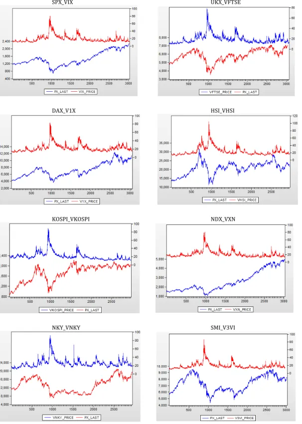
The asymmetric and negative relationship between the changes in implied volatility index and its underlying equity index for many stock markets is a well-documented fact in the literature (Giot, 2005; Fleming et al., 1995). Usually negative price movement follows by a larger increase in the volatility than the positive price movement of the same magnitude. To visualize this relationship graphically, daily closing prices of equity index for the full sample period is plotted along with its volatility index levels for the 10 equity indices in Appendix, Figure 1. As the graphs clearly show, there seems to be a negative correlation between the equity index levels and its model-free implied volatility levels and for many of the indices there also seems to be asymmetric relationship between the two.
Table III illustrates the descriptive statistics of the daily range-based series using the Parkinson (1980) price range estimator and its daily scaled model-free implied volatility series of the sample period 1/3/2005 – 12/30/2016 for the 10 stock indices. Across all indices, the range-based time series and its implied volatility series exhibit positive
skewness and large excess kurtosis. As a result, Jarque-Bera test of the normality is rejected for all instances even at 1% significance level.
5.2 Out-of-Sample Forecast Evaluation
Using the 4 loss functions (RMSE, MAE, MAPE and Theil’s U Statistic)
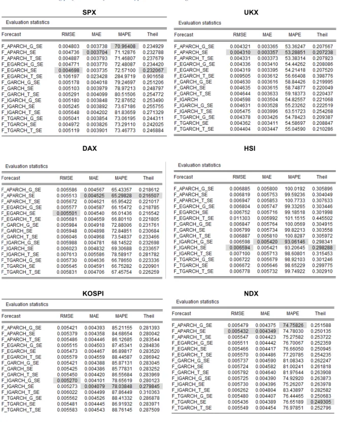
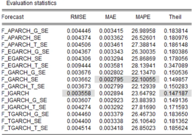
aforementioned, the forecasting accuracy of the various GARCH (1, 1) type models with Normal, Student-t and GED innovations are scrutinized against range-based estimator and implied volatility as proxies of ex-post volatility and the findings are summarized in the table below. More detailed outputs of EViews test results are included in the appendix, Table IV and V where model with the lowest forecasting errors for each loss function is highlighted in grey. The model with best 1-day ahead out-of-sample forecasting
performance is assessed with the values of RMSE, MAE, MAPE and Theil’s U Statistics. Table II: Forecasting Performance Summary
Equity Index “Best” Models (Range Volatility) “Best” Models (Implied Volatility)
SPX EGARCH (Normal) GARCH (Student-t)
UKX APARCH (Normal) GARCH (Normal), IGARCH (Normal) – RM
DAX APARCH (Normal) GARCH (Student-t)
HSI IGARCH (Normal) – RM, IGARCH (GED) GARCH (Student-t), APARCH (Student-t)
KOSPI IGARCH (Normal) – RM GARCH (Student-t)
NDX APARCH (Normal) GARCH (Student-t)
NKY APARCH (Student-t) GARCH (Student-t)
SMI APARCH (Student-t) GARCH (GED)
SX5E APARCH (Normal) GARCH (Student-t)
CAC APARCH (Normal) GARCH (Student-t)
As the 4 loss functions were designed differently in measuring the deviation from the observed value, it is not common to one model that uniformly beats the others across all criteria. For instance, RMSE is said to be scale-dependent measure and is more sensitive to the large deviation than the sum of smaller deviations even if the total deviations are the
same, while MAE is also scale-dependent, but it is considered to be less sensitive to larger deviation in comparison to RMSE. The method of selecting the best model(s) of each time series is based on at least two or more loss functions.
Based on table II, in forecasting range estimator the results are rather mixed; generally, asymmetric GARCH type model (1,1) such as APARCH (1,1) seem to adequately capture the dynamic of the future volatilities across 7 of 10 indices. This coincides with Poon and Granger’s (2003) conclusion that models account for volatility asymmetry generally performs well. Within these indices, when taking into consideration of distribution variations, normal distribution can explain 5 of 7 indices while Student-t innovation explains the other two indices namely NKY (Japan) and SMI (Switzerland). This result is in line with another research conducted by Brownless et al. (2011), where the authors found Student-t innovation generally did not yield any improvement in the
performance of the models across a wide variety of asset classes. It seems that NKY and SMI are the exceptions, which suggests that realized volatility obtained using range-based estimator exhibits heavier tails compared to the other indices chosen. RiskMetrics
methodology using IGARCH (1,1) normal distribution as a proxy gains competitive edge in forecasting realized volatility of HSI (Hong Kong) and VOSPI (Korea) indices. On the other hand, when forecasting realized volatilities using model-free implied volatilities across 10 indices, simple symmetric GARCH (1,1) seems to perform well overall. This result suggests that market participants seem to weight positive and negative price movements symmetrically in their perceived future risk. When drilling down to the
different distribution assumptions, Student-t innovation performs relatively well for 8 of 10 indices, normal and GED are suitable for UKX (U.K) and SMI (Switzerland) respectively.
5.3 Information Content Regression Result
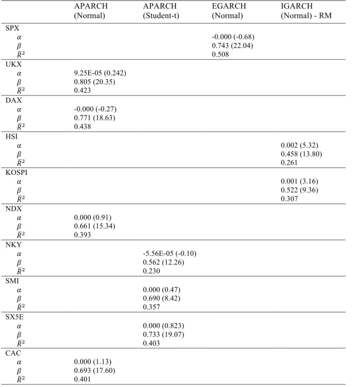
The best forecasting model from each category (Range-based estimator and MFIV) of each index is then selected in the univariate regression analysis using ordinary least square (OLS) method based on equation 25 to see if they also contain some information about the future volatility in addition to their forecasting accuracy. To account for heteroscedasticity and autocorrelations of residuals of the regression, Newey West correction of standard error procedure is used in EViews with automatic selection of lag length option.
Before running the univariate regression, Augmented Dickey-Fuller Unit Root test is done on all the time series to eliminate the uncertainty of possible spurious regression problem with non-stationary time series. All time series presented in the regression are able to reject the null hypothesis of a unit root at less than 5% with the exceptions of implied volatility time series of HSI and RiskMetrics model for HSI, where the rejections of unit root are at 8.5% and 7.2% respectively.
In Appendix, Table VI and VII illustrate the results of the univariate regression analysis on range-based estimator and model-free implied volatility respectively. Both constant coefficient (𝛼) and slope coefficient (𝛽) with its corresponding T-statistics in parentheses of each model are reported along with 𝑅!. It is evident that all slope coefficient
estimates are different from 0 and statistically significant at less than 1%, which provides evidence that all forecasts bear some information about the future volatility.
Finally, using the same regression can also test the unbiasness of the time series forecasts through the joint hypothesis 𝛼=0 and 𝛽=1 using Wald F-statistic in EViews. The
results show that at every instance, the null hypothesis can be rejected at less than 1%. This provides statistical evidence that all volatility forecasts presented in this study are
somewhat biased, which is in line with the conclusion from Jiang and Tian (2005) and Andersen et al. (2007b) that most volatility forecasts seem to be somewhat biased.
6 Conclusions and Future Research
The main purpose of this thesis is to investigate the forecasting performance of various GARCH models with different innovation assumptions (Normal, Student-t and GED) against the range-based estimator and implied volatility as proxies for realized volatilities in a more global context by using 10 frequently traded equity indices and its volatility indices. In this study, Parkinson (1980) range-based estimator is used to represent the ex-post “realized” volatility due its unbiasness and it is believed to be 5 times more efficient as the squared return measure according to Garman and Klass (1980). On the other hand, model-free implied volatility index from each exchange is used to represent market’s expected future volatility, which is another proxy for ex-post volatility. As many prior researches state that implied volatility contains important information about future ex-post volatility and it is the markets best guess of what will happen in the near future. Model-free implied volatility does not depend on any econometrics model and it does not subject its calculation to any distribution assumption of the stock prices and returns unlike the popular Black-Scholes equation. In order to assess the forecasting error of each model overtime, fixed rolling window method is employed with 1,000 observations for each in-sample estimation covering over 10 years of data (1/3/2005 – 12/30/2016) and the accuracy of each
forecast is evaluated with the four loss functions (RMSE, MAE, MAPE and Theil’s U statistic).
Although the results are not clear-cut, there are some patterns observed. Depending on the index, in forecasting the ex-post volatility, overall asymmetric model such as APARCH (1,1) with Normal innovations is the one with best performance with the exceptions of NKY (Japan) and SMI (Switzerland) where Student-t innovation performs better. RiskMetrics methodology excels in forecasting ex-post volatility of HSI (China) and KOSPI (Korea) index. As volatility has many characteristics, some characteristics might be more pronounced in one index over the others. For instance, it seems that heavy kurtosis such as Student-t can describe NKY and SMI relatively well, which implies that realized volatility from these two indices might be more heavy-tailed comparing to others. The results from forecasting implied volatility are more consistent in terms of the type of
GARCH model that can capture the market’s expected volatility across 10 indices; a simple GARCH (1,1) with Student-t innovation seems to perform relatively well with exceptions of UKX (U.K) and SMI (Switzerland) where Normal and GED seem to perform better. This result from forecasting implied volatility seems to imply that market participants seem to weight positive and negative price shocks equally in their perceived future expected risk. Finally, through univariate regression analysis, it shows that all the winner models bear some information about future volatility (range-based estimator and MFIV). The regression analysis also suggests that all the forecasts are somewhat biased, which is in line with many other prior researches that suggest many volatility forecasts are biased. Fleming (1995) concludes that while unbiasness is a good property, it is not the most crucial property if the degree of biasness can be pinpointed and corrected.
Although this thesis provides a good overview of the forecasting ability of various GARCH (1,1) models across 10 global equity indices, it can be extended to include higher order GARCH (m, n) models and long memory time series models proposed in the recent literature such as the Fractional Integrated GARCH (FIGARCH) and Heterogeneous Autoregressive Model (HAR) to forecast future volatility. In a study conducted by Martens and Zein (2004), the authors conclude that long memory models such as the Fractional Integrated GARCH model dramatically change the result of the contest between time series model and implied volatilities. Kourtis et al. (2016) report the success of using
Heterogeneous Autoregressive model (HAR) in one-day ahead forecasts for realized volatilities compared to GJR-GARCH model. In addition of incorporating more variety of the time series models to forecast the future volatility, the sample period in question could also be divided into different sub-periods, for example, to analyze how the various model perform during period of high distress such as late 2008 – 2009.
Bibliography
Akgiray, V. (1989). Conditional Heteroskedasticity in Time Series of Stock Returns: Evidence and Forecasts. Journal of Business , pp. 62, 55-80.
Andersen, T. G., Frederiksen, P., and Staal, A. (2007). The Information Content of
Realized Volatility Forecasts. Northwestern University. Working paper.
Andersen, T., and Belzoni, L. (2008). Realized Volatility. Working paper , 2008-2014. Federal Reserve Bank of Chicago.
Andersen, T., and Bollerslev. (1998). Answering the Skeptics: Yes Standard Volatility Models do Provide Accurate Forecasts. International Economic Review , pp. 39: 885-905.
Blair, B., Poon, S.-H., and Taylor, S. J. (2001). Forecasting S&P 100 Volatility; The Incremental Information Content of Implied Volatilities & High Frequence Index Returns.
Journal of Econometrics , pp. 5-26.
Bollerslev, T. (1986). Generalized autoregressive conditional heteroscedasticity.
Journal of Econometrics , pp. 307-27.
Brace, A., and Hodgson, A. (1991). Index Futures Options in Australia - An Empirical Focus on Volatility. Accounting & Finance , pp. 13-31.
Brook, C. (2008). Introductory Econometrics for Finance. Cambridge University Press.
Brownless, C., Engle, R., and Kelly, B. (2011/12). A practical Guide to Volatility Forecasting Through Calm and Storm. The Journal of Risk , pp. 3-22.
Canina, L., and Figlewski, S. (1993). The Informational Content of Implied
Volatility. Review of Financial Studies , pp. 689-81.
Cumby, R., Figlewski, S., and Hasbrouck, J. (1993). Forecasting Volatilities and Correlations with EGARCH Models. Journal of Derivatives , pp. 51-63.
Demeterfi, K., Derman, E., Kamal, M., and Zou, J. (1999). More than you ever
wanted to know about volatility swaps. Goldman Sachs.
Ding, Z., Engle, R., and Granger, C. (1993). A long Memory Property of Stock Market Returns and A New Model. Journal of Empirical Finance , 1, pp. 83-106.
Doidge, C., and Wei, J. Z. (1998). Volatility Forecasting and the Efficiency of the Toronto 35 Index Options Market. Canadian Journal of Administrative Science , pp. 28-38.
Dupire, B. (2004). Arbitrage Pricing with Stochastic Volatility. Derivatives Pricing, pp. 197-215.
Dupire, B. (1994). Pricing with A Smile. Risk , pp. 18-20.
Engle, R. (1982). Autoregressive Conditional Heteroscedasticity with Estimates of the Variance of United Kingdom Inflation. Econometrica , pp. 987-1008.
Exchange, C. B. (2003). VIX CBOE Volatility Index. Retrieved March 25, 2017, from CBOE: http://www.cboe.com/micro/vix/introduction.aspx
Figlweski, S. (1997). Forecasting Volatility. Financial Markets, Institutions &
Instruments , pp. Vol. 6, No. 1, p. 1-88.
Fleming, J., Ostdiek, B., and Whaley, R. E. (1995). Predicting Stock Market Volatility. Journal of Futures Markets , pp. 265-302.
French, K. R., William, S. G., and Stambaugh, R. F. (1987). Expected Stock Returns and Volatility. Journal of Financial Economics , pp. 3-30.
Frennberg, P., and Hansson, B. (1996). An Evaluation of Alternative Models for Predicting Stock Volatility. Journal of International Financial Market, Institutions and
Money , pp. 117-34.
Garman, M. B., and Klass, M. J. (1980). On the Estimation of Security Price Volatilites from Historical Data. Journal of Business , 53, pp. 67-78.
Giot, P. (2005). Relationship Between Implied Volatility Indexes and Stock Index Returns. The Journal of Portfolio Managment , pp. 92-100.
Glosten, L., Jagannathan, R., and Runke, D. (1993). On the Relation between the Expected Value and the Volatility of Nominal Excess Return on Stocks. (48(5), Ed.) The
Journal of Finance , pp. 1779-1801.
Hentschel, L. (1995). All in The Familiy: Nesting Symmetric and Asymmetric GARCH Models. Journal of Financial Economics , pp. 71-104.
Hull, J. C. (2014). Options, Futures and Other Derivatives (9th Edition ed.). Prentice Hall.
Hyndman, R., and Koehler, A. (2006). Another Look at Measures of Forecast Accuracy. International Journal of Forecasting , 22, pp. 679-688.
Jiang, G., and Tian, Y. (2005). The Model Free Implied Volatility and its Information Content . Review of Financial Studies , 18 (4), pp. 1305-1342.
Kourtis, A., Markellos, R. N., and Symeonidis, L. (2016). An International Comparison of Implied, Realized and GARCH Volatility Forecasts. Journal of Futures