ENVELOPES OF COMETARY ORBITS
ˇ
Z. Mijajlovi´c1, N. Pejovi´c2, G. Damljanovi´c3 and D. ´Ciri´c4 1Faculty of Mathematics, University of Belgrade
Studentski trg 16, 11000 Belgrade, Serbia E–mail: [email protected]
2Department of Astronomy, Faculty of Mathematics, University of Belgrade Studentski trg 16, 11000 Belgrade, Serbia
E–mail: [email protected]
3Astronomical Observatory, Volgina 7, 11060 Belgrade 38, Serbia
E–mail: [email protected]
4Faculty of Natural Sciences and Mathematics, University of Niˇs, Viˇsegradska 33, 18000 Niˇs, Serbia
E–mail: [email protected]
(Received: July 16, 2008; Accepted: September 5, 2008)
SUMMARY: We discuss cometary orbits from the standpoint of Nonstandard (Leibnitz) analysis, a relatively new branch of mathematics. In particular, we con-sider parabolic cometary paths. It appears that, in a sense, every parabola is an ellipse.
Key words. Comets: general – Methods: analytical
1. INTRODUCTION
The standard approach to physics is based on mathematics overR, the field of real numbers, orC, the field of complex numbers. Both these structures are Archimedean, i.e. they do not admit explicitly infinite quantities. In discussing the real lineR we have no way of knowing what a line in physical space is really like. It might be like the real lineR, the hy-perreal line∗Rwhich contains infinitesimals and
in-finite numbers, or neither. However, in applications of the mathematical analysis it is helpful to imagine a line in a physical space as ∗R. The hyperreal line is, like the real line, a useful mathematical model for a line in the physical space. One of the aims of this paper is to advocate the use of methods from non-standard analysis (also known as Leibnitz analysis, non-Archimedean analysis or Robinson’s analysis) in studies of certain phenomena in astronomy. Here we shall discuss trajectories of comets.
2. NONSTANDARD ANALYSIS
It is generally accepted that Newton and Leib-nitz, independently from each other, developed dif-ferential calculus. By infinitesimals Leibnitz as-sumed ”infinitely small numbers”, and he performed the usual algebraic operations over them in the same way as he did with real numbers. In particular, each positive infinitesimal ε in this contemplation was lesser than any ordinary real (standard) positive number, while 1/ε was greater than any standard positive number. The following rule was implicitly supposed:
Leibnitz principle: Every mathematical proposi-tion that is true for finite (real) numbers is also true for the extended system (i.e. system with infinite numbers), and vice versa.
The major difficulty of Leibnitz’s approach was a number of paradoxes and a lack of formal framework for consistent foundation of infinitesimal calculus. Introducing Weierstrass analysis the infi-nite quantities are expelled, for example the notion of the infinitesimal is replaced by the ε - δ formal-ism. In particular, zero-sequences (i.e. sequences that converge to 0) are seen as infinitesimals. How-ever, this is only an auxiliary notion there, and they lack the use of all algebraic operations (such as divi-sion) over them.
Abraham Robinson (1961) solved the 300 years old problem of foundation of infinitesimal cal-culus. He founded Leibnitz analysis, i.e. introduced actual infinitely small and infinitely large numbers. They admit not only all algebraical operations, but also an application of usual functions from analysis (such as sin, cos, exp etc) on them. Robinson’s so-lution was based on certain constructions and tech-niques from mathematical logic, such as the ultra-products, the Compactness theorem and the satu-rated models. The reader can find details about these notions in Chang and Keisler (1990).
The nonstandard analysis is based on proper-ties of ∗R and the transfer principle (ÃLo´s theorem), the counterpart of the Leibnitz principle, which ex-change propositions between ∗R and R. The non-standard analysis has been used since then in ex-plaining certain phenomena in physics, in particular in statistical physics and quantum mechanics (e.g. S. Albeverio, J. E. Fenstad, T. Lindstrom, see Ander-son 1976, Albeverio, et al. 1986).
Mathematical models of nonstandard analysis are Archimedean real fields enriched with non-standard counterparts of notions of the mathemat-ical analysis: elementary functions sin(x),ln(x), . . ., sets: natural numbers N, integersZ, rational num-bers Q, etc. As they are non-Archimedean, they contain infinitesimals and infinite quantities. The best of all is that we can do the same with more complex structures. For example, to construct the nonstandard enlargement of any infinite structure: complex numbersC, the space of real sequencesRN,
the space of real functionsRR, each having the
met-ric of our choice; then infinite functional, geometmet-rical and topological spaces. This construction simply
al-lows us to do nonstandard but consistent mathemat-ics. Leibnitz transfer principle enables one to trans-late theorems expressed by special, so called internal formulas from nonstandard universe to the standard one. In particular, the Cauchy transfer principle is useful in such translations:
The Cauchy PrincipleLetϕ(x) be an internal for-mula. Then: If ϕ(x)holds for each infinitesimal x, then there isr∈R, r >0, such thatϕ(x)holds inR
for all x∈R,|x|< r.
Let us mention few facts about nonstandard analysis: by ∗R we shall denote some ℵ1-saturated non-Archimedean (in the sense of order) elementary extension of the ordered field of realsR. Though ℵ1-saturation provides uniqueness (up to isomorphism) at the given cardinal number of such structures, we do not have the canonical representation (such as decimal notation for reals) of nonstandard real num-bers. Another useful property is expressed by the following theorem
Theorem (Extension property) Every function
f:R−→R can be extended to ∗f:∗R−→∗R which preserves all first order properties of f.
For example, if f(x) = sin(x), g(x) = cos(x), since
sin(x+y) = sin(x) cos(y) + cos(x) sin(y),
the same identity holds for ∗f(x) = ∗sin(x) and ∗g(x) = ∗cos(x). Something similar is true for an-alytical continuations of real functions, but only for identities. In nonstandard analysis all the first or-der properties are preserved, including monotonic-ity, properties of zeros, etc. It is customary that the asterisk∗ is omitted in the case of elementary func-tions. Thus, sin(x) will denote ∗sin(x) if x ∈ ∗R, otherwise it is the ”ordinary” sinus function.
Another useful notion in nonstandard analy-sis are monads. An element a∈∗R isfinite if there is a positive integer n such that −n < a < n. By ∗R
f inwe shall denote the set of all finite elements of
∗R. The galaxy of a is the set g(a) of all nonstan-dard reals b such that a−b is finite. In particular, ∗R
f in = g(0). It is easy to see that the mapping
st:∗R
f in−→R (standard part) defined by
st(x) = sup
R
{y |y6x}
is an epimorphism. In particular,∗R
f in/ker(st)∼=R.
An infinitesimal is each finite ε such that st(ε) =
st(0) = 0. The monad of 0 is the set µ(0) of all infinitesimals. Notice thatµ(0) is closed under addi-tion and multiplicaaddi-tion. Further, we say thataandb
areinfinitely close, denoted bya≈b, ifa−b∈µ(0). In fact, µ(0) is a kernel of epimorphism stand it is a maximal ideal of the ring ∗R
f in. We get the other
monads by translations, i.e. µ(a) =a+µ(0).
Examples from mathematics
1. Ifεis an infinitesimal, thenst(a+ε) =st(a). 2. f:R−→Ris continuous iff (if and only if) for all
a∈∗R
f in,st(∗f(a)) =f(st(a)).
3. f:R −→ R is uniformly continuous iff for all
a, b∈∗R,a≈b→∗f(a)≈∗f(b).
4. Let f:R −→ R be a differentiable function and let ε 6= 0 be an infinitesimal. Then f′(x) =
st³∗f(x+εε)−f(x)´. For example,
(x2)′=st
µ
x2+ 2xε+ε2−x2 ε
=st(2x+ε) = 2x.
5. Every subsetSofRhas the nonstandard enlarge-ment∗S. IfSis finite then∗S=S, but ifSis infinite then∗S\S is also infinite.
6. Iff is continuous, then the Riemann integral may be defined, for example
1
R
0
f(x)dx = 1
H H
P
i=0
∗f(i/H),
whereH is an infinite number, i.e. H∈∗N\N. One can find detailed development of nonstan-dard analysis in Stroyan and Luxemburg (1976).
Examples in Geometry and Astronomy. Non-standard analysis, based on∗R, introduces a specific mathematical method, as well as a way of thinking. As we saw, it introducesactualinfinitely small quan-tities and infinitely large quanquan-tities. Therefore, it gives good ground in considering physical systems which in idealized form have infinitely many degrees of freedom. Definitions and proofs are more intu-itive, and its use is natural and intuitive whenever the considered (idealized) physical system is com-posed of infinitely many particles. There are a lot of applications of nonstandard analysis based on this assumption in mathematical physics, in particular in quantum mechanics, fluid mechanics, dynamical sys-tems, etc. As an example, let us first consider Dirac delta function.
1. Dirac δ function Let a(t) = e−1/(1−|t|2)
if |t| < 1, a(t) = 0 otherwise. This is a simple vari-ation of Cauchy’s flat function, and it belongs to the space E∞ of infinitely many differentiable func-tions. Let ε be a positive infinitesimal, and let
b(t) = a(t/ε). Finally, let k = R∞
−∞b(t)dt and let
δ(t) =b(t)/k=a(t/ε)/k.Thenδ(t) belongs to ∗E∞, it is positive, and has integral one. In fact, this is what is expected, δ(t) is a finite compact distribu-tion and it has all properties attributed to the Dirac function.
2. Tiling the Euclidean plane, Hao-Wang dominoes problem: if there is a covering by the certain pattern of the finite typeτ of each bounded domain in the plain such as squares and circles, prove that there is a cover of the typeτof the entire plane. One solution goes like this: by the extension princi-ple, we can find the covering C of the type ∗τ of a square with edges having the infinite length H, i.e.
H ∈∗N\N. Sinceτis finite, we have∗τ=τ. There-fore, this particular nonstandard cover induces the covering of the entire Euclidean plane by restricting C to the standard (finite) part of∗R×∗R.
In this example we have seen how to extend certain local property to the global one. We can try to interpret this covering property to the founda-tion of fundamental cosmological principles. Namely, all observations from the Earth are local, even on the large scale. But observations on the large scale show that the Universe is homogeneous and isotropic. Identifying observations with tiling, we see at once that we may assume two basic cosmological prin-ciples: homogeneity and isotropy of the Universe. Therefore, from the mathematical point of view at least it is consistent to assume so.
Consistency and conservativeness of nonstan-dard analysis. Nonstandard analysis is a consis-tent and conservative extension of classical analy-sis. This follows from the ultraproduct construction (consistency), and ÃLo´s theorem (conservativeness). Nonstandard analysis cannot produce propositions in the classical mathematical analysis that are not possible to prove by means of classical mathematics. Thus, nonstandard analysis is a method of proving, first of all. However, we should mention that some problems, such as Bernstein-Robinson theorem on polynomial operators, were first solved by means of nonstandard analysis.
There are other mathematical non-Archimedean methods that are used in physics. Par-ticularly popular in last two decades becamep-adic physics, which is based on the so calledp-adic math-ematics. It admits counterparts of all basic notions of classical analysis, but they are not true extensions of standard functions of classical analysis. Also, it lacks the transfer principles such as the Leibnitz transfer principle, or they are much weaker, such as the Hasse-Minkowski theorem for Henselian fields. Without any intention to doubt the trustiness on
p-adic physics, it certainly gives interpretation of physical phenomena that differs from those in the main-stream physics. Detailed discussion on this topic one can find in Mijajlovi´c et al. (2006), Mija-jlovi´c and Pejovi´c (2007), MijaMija-jlovi´c et al. (2007).
3. ELLIPSE IN THE
NONSTANDARD UNIVERSE
Let E be an ellipse having foci at the points (p,0) and (q,0) where p > 0 is a fixed positive real number and q >0 is an infinite real number. Then all standard points ofE, i.e. the points lying in the real planeR2, are the points of loci of an ”ordinary” parabolaP having the focus at (p,0). We show that
P is actually the envelope of the family of all (stan-dard) ellipses having one focus in (p,0), the other one in (b,0), b > pis a positive real number.
From the stated assumptions on the ellipseE, see Fig. 1, we infer the following formulas:
l1+l2 = d
l2
1 = (x−p)2+y2,
l2
2 = (x−q)2+y2.
(1)
From these equations it follows
l1 = ((q−p)x+pd)/d,
l2 = ((p−q)x+qd)/d.
By eliminatingl1andl2from the set of formulas (1), we obtain finally the equation of the ellipseE:
y2= 4px−4pp(p+q)x+qx
2
(p+q)2 (2)
We can interpret the formula (2) in the following two ways.
Fig. 1. The ellipse having the foci respectively in (p,0)and(q,0)with the vertex at the coordinate ori-gin and l1+l2 =d, d=p+q, where l1 and l2 are distances of a point on the ellipse from the foci.
1. Ellipse in the nonstandard plane. Assume that p ∈R and that x∈ ∗R is finite and q ∈∗R is infinite. Then the term
4pp(p+q)x+qx
2
(p+q)2 (3)
is an infinitesimal, while 4px is finite. Hence y is also finite and y2 ≈ 4px. Thus, st(y)2 = 4pst(x), so by replacing st(x) byxand st(y) byy we obtain the equation y2 = 4px of a parabola. Therefore, the standard part of the ellipseE (see Fig. 2) in the nonstandard plane with the finite focus (p,0) and the infinite focus (q,0) is the confocal parabolaP deter-mined by the equation y2 = 4px. Observe that P does not depend on the choice of the infinite focus (q,0).
All geometric and differential properties of the parabolaP can be derived from the properties of the ellipseE. For example, the optical property that if a ray of light travels parallel to the symmetry axis of a parabola and strikes the concave side of the parabola, then it will be reflected to the focus follows immedi-ately from the corresponding optical property of the ellipseE. Just note that if a rayr′ is coming from
Fig. 2. The ellipseE in the nonstandard plane. the infinite focus (q,0) it reflects from the ellipse to the focus (p,0). Then the standard partr=st(r′) = {(st(x), st(y)): (x, y) ∈ r′, x, y ∈ ∗R
f in} is a
(stan-dard) ray parallel to thex-axis and asris infinitely close tor′ it also enters into the focus.
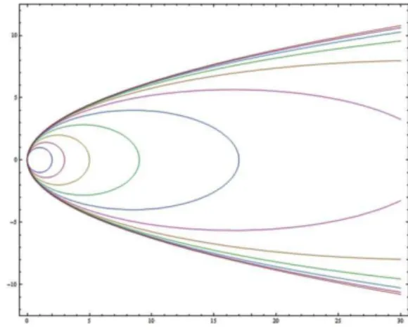
2. Family of confocal ellipses. We may take (2) as the equation of the family of (standard) ellipses sharing the fixed focus (p,0), while the second focus (q,0) runs over thex-axis. Observe that from the as-trodynamics point of view this family of ellipses may be regarded as Hohmann-Vetchinkin transfer orbits connecting co-planar circular orbits.
Fig. 3. Family of confocal ellipses.
The parabola P is the limit curve enveloping ellipses (see Fig. 3) from this family. In the classi-cal approach in mathematiclassi-cal analysis, the existence of the limit curve is guaranteed by the Arzel`a-Ascoli theorem applied in theL2 space.
However, it should be mentioned thatP is not the envelope of the family of ellipses given by the Eq. (2) as it is defined in mathematical analysis. Namely, if a family of plane curves are given by a formula
F(x, y, q) = 0,qis a parameter, then the envelope of this family is a curve osculating each member of the family. The equation of the envelope is obtained by elimination ofq from the system of equations
F(x, y, q) = 0, ∂F(x, y, q)/∂q= 0.
In our case,
4. COMETARY TRAJECTORIES
First studies of cometary orbits serve as a his-torical introduction to astrodynamics. Namely, their trajectories are also influenced by non-gravitational forces, for example by the acceleration resulting from ejection of a jet of a material from the comet. Most cometary orbits are very elongated. Many physical quantities related to the very elongated cometary or-bits change by several orders of magnitude. Every cometary orbit which is observed as parabolic actu-ally is elliptical as further calculations usuactu-ally show. If this is not the case, this is due to the fact that the second focus is too remote to measure it. Therefore, nonstandard analysis could be the appropriate math-ematical tool in the study of cometary trajectories. In the rest of this article we shall use the terminology of nonstandard analysis and the wordsstandardand infinitesimal will have meaning as explained in the previous sections. For example, if the value of the velocity at the perihelion is assumed to be standard, then the velocity at aphelion may be taken as an in-finitesimal. In particular, we shall discuss parabolic paths. By our consideration in the previous section we may assume that every parabolic trajectory is an ellipse. Our discussion is relied on available cometary data, so we shall first shortly review them.
The number of observed comets is rapidly growing due to the development of space technology. For example The ESA/NASA SOHO spacecraft, http://sohowww.nascom.nasa.gov, discovered ex-actly 1500 comets since 1995, the last one 27. June 2008 when this paper was submitted. About 2300 comets are catalogued, even if it is believed that there are more than 109of them. As very few comets have periods less than 12 years, their trajectories are good illustration for very elongated or nearly parabolic el-lipses. Here is the short history on comet discoveries in the last four decades.
According to Baker and Makemson (1960), in 1960, of the 1000 comets for which orbits have been computed, fewer than 100 had periods of revolution less than 100 years. Some 40 or 50 had periods be-tween 100 and 1000 years, and the periods of the rest were very uncertain. Fewer than 30 comets were known to have been observed on two or more returns to the Sun. About 50 comets had periods less than 12 years (Jupiter family).
The Catalog of Cometary Orbits, compiled by Marsden, 1989 edition, lists 1292 computed orbits from 239 BC to AD 1989; only 91 of them were com-puted using the rare accurate historical data from before the 17th century. More than 1200 are, there-fore, derived from cometary passages during the last three centuries. Sets of orbital elements in Marsden’s catalog involve only 810 individual comets; the re-mainder represents the repeated returns of periodic comets. Four of these comets had been definitely lost, and three more were probably lost, presumably because of their decay due to the solar heat. Of the 155 short-period comets, 93 have been observed at two or more perihelion passages.
The 16th edition of the Catalogue of Cometary Orbits of Smithsonian Astrophysical Ob-servatory issued in 2005 contains 3031 sets of orbital
elements (in the J2000.0 system) for 2991 cometary apparitions of 2221 different comets through mid-August 2005. There is a special tabulation giving osculating elements for the 170 designated periodic comets, excluding seven deemed to be lost.
According to the list of periodic comets on the Planetary Data System Small Bod-ies Node, NASA, last update on 10 April 2008, http://pdssbn.astro.umd.edu/comet data, there are 420 designated periodic comets. Ac-cording to Seiichi Yoshida’s Comet Catalog, http://www.aerith.net/, there are 243 non-designated periodic comets (the last discovered C/2008 L3, 13. Jun 2008) and 200 designated pe-riodic comets.
In discussion of very elongated cometary or-bits we shall rely on Marsden Catalog of Cometary Orbits. Of the 655 comets of long period contained in the Catalog, 192 have osculating elliptic orbits, and 122 have osculating orbits that are very slightly hy-perbolic. Finally, 341 are listed as having parabolic orbits, but this is false because either it has not been possible to detect unequivocal deviations from a parabola on the usually very short arc over which the comets have been observed or the final calcula-tions have never been made. However, the parabola is always assumed first in the computation of the pre-liminary orbit. If the osculating orbit is computed backwards to when the comet was still far beyond the orbit of Neptune and if the orbit is then referred to the centre of mass of the solar system, the original orbits almost always prove to be elliptic.
These data show that the methods of nonstan-dard analysis are suitable in studying of cometary trajectories. For example, in the computation of the preliminary orbits, the value of the parameter p is computed. Simply, the second term (3) in Eq. (2) may be omitted as we may consider it as an infinites-imal. It also shows that the formula (2) could be very appropriate in calculation of cometary orbits in the sense that it represents better starting point for the method of differential corrections than the simple parabola.
Let us consider very-long-period comets and comets having orbits not significantly different from a parabola. It is believed that these comets orig-inate in the Oort cloud which is located 10000 and 100000 AU from the Sun. By our previous discussion it is appropriate to use here methods of nonstandard analysis. So let us assume that a hypothetical comet
C is moving along an ellipse E in the nonstandard plane having the second focus at (q,0) where q is an infinite number. Therefore, the aphelion of E is at infinity, and by the second Kepler’s law the ve-locity v of the comet near the aphelion (i.e. at the finite distance from aphelion in terms of nonstandard analysis) is an infinitesimal. Otherwise, the surface swept by the comet for the finite time △t would be infinite due to the infinite distance of the comet from the Sun, and that would contradict the Second Ke-pler’s law. In reality, a simple calculation shows that the velocityvof the cometCnear aphelion would be around 100 m/sec, negligibly small comparing to the velocity at the perihelion. Therefore, the momen-tump=mv of the cometC is an infinitesimal too;
we could say that the comet C floats in the Oort cloud instead of travelling around the Sun. Hence the trajectory of the comet C is subject to a very small perturbation. We show that an infinitely small force, or impulse, would change significantly its tra-jectory. Simply saying, parabolic orbits at large dis-tances are very unstable. We can see that using the following formula from astrodynamics (see Andjeli´c 1983, pages 132-134):
vat = s
2µ ρa2
ρp1 ρp1+ρa2
(4)
which determines the velocity vat needed for the
bodyC to continue travelling along the other orbit which is coplanar and confocal toE.
So let O2 be the orbit E with the apoapsis
ρa2 along which the body C travels so that C is at
the aphelion (i.e. in the Oort cloud) with the in-finitely small velocity vC. Further, let O1 be the orbit, coplanar and confocal toO2, with the periap-sisρp1to which the bodyCwill be transferred under
an actionA. Observe thatρa2 is infinite, whileρp1 is
finite. According to the Maupertuis’ principle of the least action, we may assume that the transition path fromO2toO1will be the Hohmann transfer orbitH touching the orbitO1 at the aphelion, so the equa-tion (4) can be applied. Here,µis the gravitational parameter andvat is the velocity resulting from the
actionA. Under these assumptions, we have
vat = p
2µρp1 ρa2
(1− ρp1
2ρa2
+ ε
ρa2
)
whereεis an infinitesimal. Simplifying the previous formula, we findvat =
p
2µρp1/ρa2−κ/ρ2a2, where κis a standard finite value. Observe that vat is an
infinitesimal of the order 1/ρa2.
Letva2=vC be the velocity of the bodyCat
the aphelia on the orbitO2. Thenvδ =va2−vat is
the velocity needed for transition from the orbitO2 to the transfer ellipse which would carry the comet
C to the orbit O1. Since va2 and vat are
infinitesi-mals, it follows thatvδ is an infinitesimal, too. The
transfer ellipse H with the second focus at infinity will be seen from the near neighborhood of the Sun as a parabola.
There are astronomical evidences that sup-port our discussion. Namely, according to Delsemme (2008) among the very-long-period comets, there is a particular class of comets that Oort showed as having
never passed through the planetary system before, notwithstanding the fact that their original orbits were elliptic, which implies repeated passages. This paradox vanishes when it is understood that their perihelia were outside of the planetary system be-fore their first appearance but that their orbits have been perturbed while they resided near aphelia, ei-ther by stellar or dark interstellar-cloud passages or by galactic tides, in such a way that their perihelia were lowered into the planetary system.
REFERENCES
Albeverio, S. et al.: 1986, Non-standard Methods in Stohastic Analysis and Mathematical Physics, Academic Press, New York.
Anderson, R. M.: 1976, A non-standard representa-tion for Brownian morepresenta-tion and Ito integrarepresenta-tion, Isr. J. Math,25, 15-46.
Andjeli´c, T. P.: 1983, An introduction to Astrody-namics (in Serbian), Mathematical Institute, Belgrade.
Baker, R. M. L., Makemson, M. W.: 1960, Astrody-namics, Academic Press, New York.
Chang, C. C., Keisler, H. J.: 1990, Model Theory, North–Holland, Amsterdam.
Delsemme, A. H.: 2008, comet, Encyclopedia Bri-tannica. Ultimate Reference Suite. Chicago: Encyclopedia Britannica.
Mijajlovic, ˇZ., Miloˇsevi´c, M., Perovi´c, A.: 2006, Infinitesimals in Nonstandard Analisys ver-sus Infinitesimals in p-adic Fields, AIP Conf. Proc.,826, New York, 274-279.
Mijajlovi´c, ˇZ., Pejovi´c, N.: 2007, Non-Archimedean Methods in Cosmology, AIP Conf. Proc., 895, New York, 317-320.
Mijajlovi´c, ˇZ., Pejovi´c, N., Ninkovi´c, S.: 2007, Non-standard Representation of Processes in Dy-namical Systems,AIP Conf. Proc.,934, New York, 317-320.
Robinson, A.: 1961, Non-Standard Analysis, Proc. Roy. Acad. Amsterdam, ser. A,64, 432-440. Stern, I.: 1997, On Fractal Modeling in Astrophysics: The Effect of Lacunarity on the Convergence of Algorithms for Scaling Exponents, Astro-nomical Data Analysis Software and Systems VI, ASP Conference Series,125.
OBVOJNICE KOMETSKIH ORBITA
ˇ
Z. Mijajlovi´c1, N. Pejovi´c2, G. Damljanovi´c3 and D. ´Ciri´c4 1Faculty of Mathematics, University of Belgrade
Studentski trg 16, 11000 Belgrade, Serbia E–mail: [email protected]
2Department of Astronomy, Faculty of Mathematics, University of Belgrade Studentski trg 16, 11000 Belgrade, Serbia
E–mail: [email protected]
3Astronomical Observatory, Volgina 7, 11060 Belgrade 38, Serbia
E–mail: [email protected]
4Faculty of Natural Sciences and Mathematics, University of Niˇs, Viˇsegradska 33, 18000 Niˇs, Serbia
E–mail: [email protected]
UDK 523.64 : 521.314
Originalni nauqni rad
U radu se razmatraju kometske orbite sa stanovixta nestandardne analize, rela-tivno nove oblasti matematike. Posebno
se izuqavaju paraboliqne kometske orbite. Pokazuje se da je, u odreenom smislu, svaka parabola zapravo elipsa.