doi: 10.1590/0101-7438.2014.034.02.0251
AN EVOLUTIONARY STUDY ON CROP PRODUCTION
IN SMALL FARM SYSTEMS IN THE MID-WEST REGION OF BRAZIL BASED ON A LINEAR PROGRAMMING MODEL
Maria Amelia Biagio
Received August 22, 2012 / Accepted December 8, 2013
ABSTRACT.Based on an agro-technical study for the mid-west region of Brazil, and considering financial conditions like monthly expenses and long-term investments, a mixed integer and dynamic linear model has been proposed for representing crop production systems. This model establishes a monthly dynamic treatment of production and financial activities over a long-term planning horizon for small and medium farm systems. In this paper, by considering more recent government financial policies for the Brazilian agricultural sector related to thePronafandProgercredit lines, a mathematical model is updated for distinct situations derived from the use of short and long-term loans which were defined for small and medium farmers. In this way, new versions of the original model are obtained by separately implementing into the production systems economic and financial conditions of credit lines for the years 2006 and 2009. Computational tests are performed and the results obtained are presented in several scenarios. Also, an evolutionary analysis on the socio-economic and financial feasibility of the agricultural farm system is drawn over the last decade by comparing the results obtained to one known from the year 2002.
Keywords: agricultural production planning, family farming systems, linear programming.
1 INTRODUCTION
The economic and social importance of small and medium Brazilian farms has been drawing attention in the last decades. Particularly, the participation of small agricultural systems in the rural economy has improved when considering gross production and exportation (IBGE – Insti-tuto Brasileiro de Geografia e Estat´ıstica, 2006). An explanation for this can be found in the fact that Brazilian small farms have received special attention with the creation in 1995 ofPronaf – National Program for Family Farming – a Brazilian governmental program that offers financial support for family farms. A qualitative and quantitative analysis on the evolution of total loans thatPronaf gave to farms in the whole country and in rural regions is presented in Guanziroli (2007). This analysis, however, does not take into consideration the financial problems of farm system production as a problem related to planning decisions.
In order to search for farm-system oriented decisions in the mid-west region of Brazil, some quantitative studies, in the area of operational research, have concentrated attention on modeling a mathematical problem for crop production planning. This has been done by presenting a finan-cial emphasis and proposing technical policies. Among these, it is important to cite the works of Veloso (1990) and Veloso et al. (1997). Based on earlier studies in the literature on agricultural systems (Dalton 1982, Dent et al., 1986 and Dent, 1990), the authors of the former and latter works present a crop production planning study of farm systems in the cities of Paracatu and Formoso, respectively, both in the state of Minas Gerais, Brazil. In these studies, they consider conventional planting techniques. Moreover, the authors propose financial-economic policies for crop production systems which are based on the following suppositions: just one family mem-ber works full time; the farmer has an initial capital contribution for the first investments; and there are three hypothetical long-term credit lines which can be used, under certain financial conditions, along a planning horizon of ten years and five months. Also, these studies supposed the farmer hires seasonal labor in the months of intensive agricultural activities and accounts are balanced monthly during the first four years and annually computed for the remaining years of the planning horizon. The entire production of the farm’s crops is supposed to be sold to a cooperative group, as the farmer is a cooperative member.
Based on agro-technical aspects proposed in the studies mentioned above, and considering finan-cial aspects like monthly expenses and long-term investments, a mixed integer linear mathemati-cal model was presented by Biagio et al. (2007) for representing small and medium farm system crop production in the District of Paracatu. This model establishes a monthly dynamic treatment of production and financial activities on a long-term planning horizon for a system based on the production of soybeans, wheat, corn and rice, which are produced in a particular rotational scheme. Computational results were presented for financial data related to the year 2002.
In the present study, by considering government financial policies for small and medium farmers in the last decade, the last cited mathematical model is updated for distinct situations derived from the use of short and long-term loans for the Brazilian agricultural sector. New model versions are obtained by implementing into the original programs credit lines available in the years 2006 and 2009, separately. Simulation tests are performed for distinct scenarios and results are obtained. Also, a discussion on the socio-economic and financial feasibility of the agricultural farm system is drawn from the results obtained and additionally, those results from the year 2002 which were already presented in the literature (Biagio et al., 2007).
Within this context this article is organized in the following way: Section 2 presents a summary of the original mathematical model of the crop production planning problem in theCerrado(2007); Section 3 describes the necessary system updates for implementing the financial conditions of Brazilian credit lines in the years 2006 and 2009; Section 4 shows and describes the obtained results; Sections 5 and 6 present a discussion and conclusions, respectively, based on the results attained.
2 MATHEMATICAL MODEL SUMMARY
land, machinery, man-power, short-term and long-term loans which strongly influence the values of total income, general expenses, in addition to credits and debts that may be monthly and annually made.
During an agricultural year the work activities on the farm are determined monthly by their type of production. Consequently, once crop production is considered as a business, the farmer may control the cash of the farm in every month along the planning horizon, which also includes transference of the cash surplus, or debts, to the next monthly account balance. This last condition defines a monthly dynamic structure for the mathematical model of farm production planning. The objective of the farmer is to maximize cash surplus and to minimize the use of his credit card every month over the entire planning horizon.
Subsections 2.1, 2.2 and 2.3 below, present a general formulation of constraints on production and financial activities and the objective function, respectively, as they are considered in the original model.
2.1 System Production Conditions
As mentioned in the earlier section, the farm systems in reference are located in the mid-west region of Brazil, which is denominated as theCerrado Biome. This is an important region for the agricultural sector of the country because it has a good climate with no strong temperature changes or rainstorms and plant infestation problems are under control. Traditionally considered inappropriate for intensive cultivation, is today the area largely responsible for the agricultural exports of the country.
The Cerrado climate is characterized by two seasons: dry and rainy. The dry season occurs in the period from May to September, and the rainy season happens from October to April. In accordance with the seasons, the agricultural year in this region begins in May and finishes in the following April. Savanna is the typical regional vegetation and is marked by large areas of acid and low fertility soils, which are classified into three main types of oxisols (Latossolos): the
LVA, theLVand theLHIsoils representing 20%, 60% and 20% of theCerradoarea, respectively. Soils corresponding to typeLVare more argillaceous and better for straining than the other types.
As crop yield generally depends on both season and type of soil, with this problem it is supposed that rice, corn and soybean crops are produced inLVAandLVsoils in rainy seasons, and wheat and soybean crops are produced in irrigatedLV andLHI soils during dry and rainy seasons, respectively. In this way, the calendar of the agricultural year is defined as follows: rice, corn and soybeans may be planted in the months of October and November, and may be harvested in the months of January, March and April. Wheat crops may be planted in May and harvested in September. Moreover, soybean crop is planted in a rotation scheme with any of the other three grains in order to reach productivity improvements for the soils.
may be done between seasons when the farmer may use (owned and/or rented) machinery such as a tractor and/or harvester. Direct costs of inputs include expenditures on fertilizer, herbicides, seeds, packaging, electric energy and also permanent workers.
Just one family member manages and operates the farm full-time; i.e., he may dedicate 200 hours a month to manage and to operate production activities, which include sowing and harvesting. An additional 200 hours of seasonal family labor is foreseen for the months of intensive sowing and harvesting activities, together with the necessity of hiring seasonal working labor.
Considering the aforementioned conditions above, the planning problem is described below, which considers the production of four different types of crops subject to six necessary monthly resources and five financial instruments, along a planning horizon. The monthly resources are: tractor, harvester, management and seasonal labor working time, direct costs of inputs and gross income. The financial instruments are presented in the next section.
Costs related to soil fertility correction may be computed among the costs of inputs in the months of May and October. For notational simplicity, considered in the constraints below, there are no fertility differences among soil types (for details, see Biagio et al., 2007). In this way, the parameters and variables used for the mathematical model description are defined as follows.
Parameters:
• T is the planning horizon;
• ai,j(k)is the coefficient related to the j-th necessary resource, j =1, . . . ,6, for thei-th
crop production/hectare,i =1, . . . ,4, in thek-th month,k=1, . . . ,12;
• Lr is the loan upper bound for ther-th credit line,r=1, . . . ,5;
• I5 is the monthly interest rate of the credit card and Ir is the percentage on loan debts
updated, and related tor-th credit line,r =1,2,3,4;
• IDis the amount of money that the farmer may provide to be spent monthly on the family’s
discretionary consumption;
• Iwis the interest rate due to monetary correction on investments made with the cash surplus of the previous month.
Decision variables:
• xi(k,t)is the land area producing thei-th crop in the monthkand yeart, where rice, corn,
soybeans and wheat crops are represented by varying theiindex from 1 to 4, respectively;
• x3I(k,t)is the land area producing soybeans in irrigated soils, in the monthkand yeart;
• yj(k,t)is the j-th necessary resource in the monthkand yeart, which varies in
accor-dance with worked land area. Particularly, the problem description, below, considers the following necessary resources, for j = 1,2, . . . ,6, respectively: tractor working time, harvester working time, management working time, working time of seasonal labor, direct costs of inputs and gross income;
• zr(k,t)is the amount of money withdrawn from ther-th credit line,r =1, . . . ,5, in the
monthkand yeart;
• w(k,t)is the cash surplus in the monthkand yeart;
The inequalities (1) below, represent the constraints related to each of the necessary resources.
a1,j(k)x1(k,t)+a2,j(k)x2(k,t)+a3,j(k)x3(k,t)+a4,j(k)x4(k,t)≤yj(k,t),
for any j =1,2, . . .6, anykand 0≤t ≤T (1)
wherea1,j(k),a2,j(k),a3,j(k)anda4,j(k)are the coefficients related to the j-th resource
neces-sary for thei-th crop production/hectare (i=1,2,3 and 4), respectively, in the monthk.
With the aim of obtaining improvement in production, the soybean crop is produced in a rotation scheme with any of the other three cereal grains. Also, the land area used for planting in one year may remain with at least the same size in the next agricultural year. The rotation constraints can be written as in (2):
x1(k,t)+x2(k,t)≤x3(k,t+1)
x3(k,t)≤x1(k,t +1)+x2(k,t+1)
x3I(k,t)≤x4(k,t +1)
(2)
for any yeart, and monthkin accordance with the calendar of the agricultural year described above and satisfying the constraint on land availability, i.e.,x1(k,t)+x2(k,t)+x3(k,t)≤TL1, andx3I(k,t)+x4(k,t)≤TL2.
All of the aforementioned activities depend on financial investments. The next section explains how the financial conditions of the problem are formulated in the model.
2.2 Financial Conditions
In the crop production planning problem in reference, the farmer is assumed to be a cooperative member, and can sell the total crop production to a cooperative group. A tax of 2,5% is retained by a rural government fund, namelyFUNRURAL.
Pronaf (National Program for Family Farming) long-term credit lines and for the second it con-siders a financial package that includesProger(Program for Rural Employnment and Revenues Generation) long-term credit lines. These credit lines allow users to pay debts along a planning horizon of T years and also to pay small percentages of debts during the first four years from the draft date.
A short-term credit line is included in every financial package. This type of credit line may finance costs with inputs and/or investments for soil preparation, and credit amounts may be withdrawn in the months of May, July, September, October, November, and/or February, which depend on both the type of crops to be produced and the land area used for that. Short-term credit lines may also finance maintenance costs of machinery. Loans can be requested every two years, and debts may be paid in full in July of the year following the loan date.
The Pronaf andProger financial packages considered in this work are presented in the next section. They are composed of one short-term and up to three long-term credit lines.
In order to have a general representation of the financial conditions cited above, it is considered, in the constraints below, three long-term credit lines, which can vary according to the use of
Pronaf or Proger (Biagio et al., 2007). In this way, let zr(k,t), r = 1, . . . ,5, be as in the
following order: the amount of money withdrawn from short-term, the first, second and third term credit lines, and credit card, respectively. So, the constraints on short-term and long-term credit limits can, respectively, be represented as in (3).
k t1+2
t=t1+1
z1(k,t)≤L1, for t1=0,2,4,6
k T
t=1
zr(k,t)≤Lr, for r =2,3,4
(3)
wherekis defined according to the calendar of the agricultural yeart mentioned in subsection 2.1. The credit card upper bounds are represented asz5(k,t)≤ L5for any monthkand yeart, 0≤t ≤T.
In relation to the farmer, the problem also considers the possibility of the farmer using his/her own initial capital contribution for investment purposes and credit card for balancing the monthly accounts of the farm. The last situation may be interpreted as a monthly debt in the farm’s ac-count balance. Decisions about the amount of machinery acquired along the planning horizon are dependent on loans from long-term credit lines and the feasibility of constraints on the account balance, which are described below.
y5(k,t)+ 4
j=1
cj(k,t)yj(k,t)+I5z5(k−1,t)+ 4
r=1
Irzr(k,t−1)+w(k,t)=
= y6(k,t)+z5(k,t)+ 4
r=1
zr(k,t)+Iww(k−1,t)−ID
for any monthkand yeart,0≤t ≤T,
wherecj(k,t)is the cost related to the j-th resource unit, j = 1, . . . ,4, in the monthk and
yeart. The percentage on loan debts updated, and related toi-th credit line,Ii,i =2,3,4, may
be paid in the month of September fori = 2,3,4 (i.e., Ii = 0 fork = 9, i = 2,3,4). It is
assumed that the short-term loan debt may be paid in the month of July of the forthcoming year (i.e.,I1=0 fork=7).
As described in the sections above, the problem presents decision variables such as land area for planting rice, corn, soybeans and wheat, besides several others which are dependent on the land area worked and the type of crop production, like the following: amount of loans to be taken out from short and long-term credit lines, necessary working time of tractor, harvester, management and hiring seasonal labor, and also direct costs of inputs and gross income. The amount of acquired machinery and permanent employees hired along the planning horizon are integer decision variables in the problem. The goal of the crop production problem presented is described in the next subsection.
2.3 Objective Function
As already mentioned in the earlier section, the objective of the problem is to maximize the monthly cash surplus and minimize the monthly loan amount taken from the credit card. So, the objective function can be written as:
Maximize T
t=1 12
k=1
w(k,t)−
T
t=1 12
k=1
z5(k,t) (5)
for allkand allt, since the account balance is made in every month of the planning horizon.
The next section presents the upgrading requirements for obtaining new versions of the original model.
3 UPGRADING THE MODEL
In this paper, the original model (2007) is adapted fromPronaf andProgerfinancial packages for the years 2006 and 2009, separately, which correspond to governmental policies for the agri-cultural sector implemented throughout the last decade. To do this, several model updates are carried out, ranging from simple but important parameters to those for a partial reformulation of farm systems.
Subsections 3.1 and 3.2 respectively describe the financial conditions of thePronaf andProger
packages in reference and subsection 3.3 summarizes the updates implemented.
3.1 PronafFinancial Package
short-term one, namely Pronaf Custeio, for soil input purposes. Loans taken out from either long-term or short-long-term credit lines must be paid within eight years and five months or two years, respectively. It is possible to take out loans from both of them simultaneously.
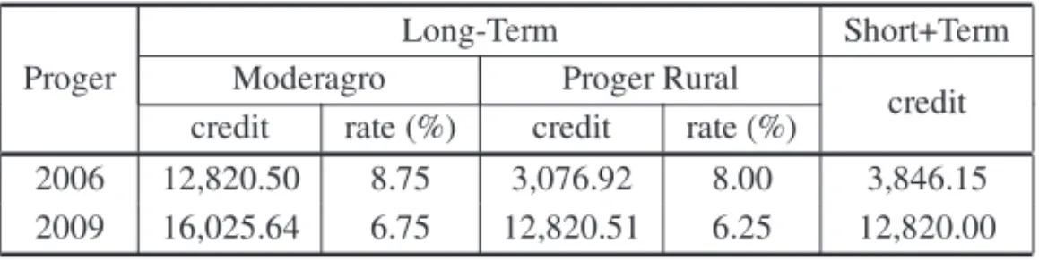
For requesting credit from Pronaf, the user must prove that his farm had an annual gross in-come average ranging from 2,564.10 u.m. to 3,846.15 u.m. in 2006 and from 1,153.84 u.m. to 7,051.28 u.m. in 2009 where u.m. is a monetary unit equivalent to US$ 7.72. Table 1, below, shows the required annual interest rates and total credit allowed by the financial packages in both 2006 and 2009.
Table 1 – Financial conditions ofPronaf in the years 2006 and 2009 (credits are in u.m.).
Pronaf Long-Term Short-Term credit rate (%) credit rate (%) 2006 2,307.7 7.25 1,794.87 7.25 2009 2,307.7 1.0 to 5.0 2,564.10 1.5 to 5.5
In 2009, the annual interest rates varied from 1,0% to 5,0% and from 1,5% to 5,5%, according to the amount of money taken from the long-term and short-term credit lines, respectively.
3.2 Proger Financial Package
As already reported, theProger financial package was created to help medium farmers and, in this study, it is supposed that medium farmers own a land area with size ranging from 60 ha to 100 ha. For both years 2006 and 2009, the Proger packages considered are composed of
Moderfrotalong-term credit lines for acquiring machines,ModeragroandProger Rural,both for general investments, and the short-term credit lineProger Custeiofor land inputs assistance. Time limits for debt payments are the same asPronaf. Table 2 below shows the amount of credit available from theModeragroandProger Rurallong-term credit lines and their respective annual interest rates in the years considered.
Table 2– Financial conditions for theProgerpackage in the years 2006 and 2009 (credits are in u.m.).
Proger
Long-Term Short+Term Moderagro Proger Rural
credit rate (%) credit rate (%) credit 2006 12,820.50 8.75 3,076.92 8.00 3,846.15 2009 16,025.64 6.75 12,820.51 6.25 12,820.00
TheProger Ruralcredit line, which includes the short-term credit lineProger Custeio, was de-fined to help farms with a gross income annual average of up to 5,128.20 u.m. in 2006 and between 7,051.28 u.m. and 32,051.28 u.m. in 2009. Loans that could be taken out simultane-ously from bothProger RuralandProger Custeiowere up to 3,846.15 u.m. and 12,820.0 u.m. in the years 2006 and 2009, respectively.
These financial rules ofPronaf andProgerrequired modifications in the original mathematical model (2007). The necessary changes are explained in the next subsection.
3.3 Reformulating the Systems
As described in subsections 3.1 and 3.2, the credit lines belonging to the 2006 and 2009Pronaf
andProgerfinancial packages offered larger loans than those in the year 2002 (see Appendix 1), bringing about the possibility of testing the feasibility of production systems in a real planning horizon. Also, they required some different financial conditions, which have to be considered in the mathematical model.
As a consequence, system reformulations must be done in the following way:
• New versions of the original mathematical model are formulated with a planning horizon of eight years and five months. As the original model (2007) was formulated with an extended planning horizon of ten years and five months, the upgraded versions present smaller systems as the number of decision variables and number of constraints in equations (1), (3) and (4) above, depend on the value of parameterT;
• Constraints related to an upper bound on joint loans fromProgershort-term and long-term credit lines are added to the mathematical system. These constraints are described by the inequalities (6) below:
t1+2
t=t1+1 12
k=1 2
r=1
zr(k,t)≤L, t1=0,2,4,6 (6)
wherezr(k,t)is the amount of money taken from ther-th credit line,r = 1,2 as
de-scribed in Section 2, and L is the upper bound on joint loans from Proger Rural and
Proger Custeio, as depicted in Table 2.
Additionally, updates on financial parameters are required and the main changes are in the following:
• For the Pronaf and Proger user, an amount of 67.3 u.m. is supposed to be withheld monthly for a family’s consumption in the year 2006. In 2006, this value corresponds to three times the monthly minimum salary in Brazil, which was of 22.43 u.m.;
• The cost of hiring seasonal work is equal to 0.12 u.m. and 0.17 u.m. an hour for the years 2006 and 2009, respectively. These values are determined by dividing the respective monthly minimum wage by 176 hours – the monthly workload in Brazil;
• The interest rates of the short and long-term credit lines are changed to the values as men-tioned in subsections 3.1 and 3.2; consequently, updates on the computations of payments and debt amounts are necessary;
• Credit card interest rate was 7,9% monthly in both years 2006 and 2009.
In consequence of the first change mentioned above, the upgraded systems present smaller di-mensions than their original ones (see Section 4 and Appendix 1), considering that the number of constraints and variables decreased, despite the addition of constraints (6) in theProger pro-grams. The obtained results are presented in the next section.
4 RESULTS
New versions of the mathematical model are obtained by applying the financial packages de-scribed above for the years 2006 and 2009, separately. They were programmed in MPS format and present systems with the following dimensions: about 1424 constraints and 2190 variables for the programs which includedPronaf packages, and about 1356 constraints and 2019 vari-ables for those includingProger packages. The computational tests were performed on aPC Pentium4, 1.80 GHz, by using the software CPLEX 9.0. The optimal values of decision vari-ables as land area designed to each crop and seasonal main labor along the planning horizon, and the computational times for running the scenarios, are showed in the tables from 9 to 20, Appendix 2. For the results, the parameterIw, in equation (4) was assumed to be 1%.
In the subsections below, tables show the results through the following notations: IC is the initial capital resource that the farmer may have for obtaining the indicated solution; TF is the total credit amount taken from the financial package long-term credit lines; ST is the annual average taken from the short-term credit line during a specified period; CC is the monthly average loan amount he may take from his credit card during a specific period of time; TL is the area of land annually used for planting, and LI is the land area annually irrigated; GI is the annual average of the gross farm income; and CS is the cash surplus of the farm at the end of the planning horizon.
In order to attain results on the economic and financial participation of the seasonal family labor in the production systems, simulation tests are also performed for two distinct supposed situ-ations: in one of them, the farmer has up to 200 monthly hours of family labor available for managing; in the second situation he has an additional 200 hours of seasonal family labor. The results are presented in the following subsections 4.1 and 4.2.
4.1 Pronaf Financial Packages
the financial packages considered for the years 2006 and 2009 are denominatedPronaf 06and
Pronaf 09, respectively.
4.1.1 No surplus family labor
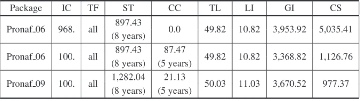
By supposing there is no additional seasonal family labor available in the months of intensive agricultural activities, the results obtained are depicted in Table 3 and described below. The word “all”, below column TF in this table, represents the maximum acceptable value shown in Table 1. Detailed information about planting area for each crop and need of hiring seasonal workers is presented in Tables 9, 10 and 11, Appendix 2.
Table 3– Financial and production results for farmers usingPronaf financial packages.
Package IC TF ST CC TL LI GI CS
Pronaf 06 968. all 897.43 0.0 49.82 10.82 3,953.92 5,035.41 (8 years)
Pronaf 06 100. all 897.43 87.47 49.82 10.82 3,368.82 1,126.76 (8 years) (5 years)
Pronaf 09 100. all 1,282.04 21.13 50.03 11.03 3,670.52 977.37 (8 years) (5 years)
As it is possible to observe, if the initial capital contribution is 968 u.m. for investments, the solution obtained for the year of 2006 indicates that the farmer could take out the whole loan amount from thePronaf long-term credit line and also an annual average of 897.43 u.m. from the short-term credit line along the eight years. In this way, by annually using a land area of 49.82 ha for planting corn, soybeans and wheat in a rotation system, the gross farm income could present an annual average of 3,953.92 u.m. and the account balance of the farm could be closed with an amount of 5,035.41 u.m. at the end of the planning horizon.
In the case of a farmer with just 100 u.m. of an initial capital contribution, the obtained solution indicates that the farmer could take the same amount of credit from thePronaf 06financial pack-age of the first case. For a land area of 49.82 ha used annually for planting rice, corn, soybeans and wheat crops, the annual average of gross farm income obtained could be 3,368.82 u.m., and the account balance of the farm could be closed with an amount of 1,126.76 u.m. at the end of the planning horizon. Additionally, in order to obtain these results, the farmer would have to use a monthly average amount of 87.47 u.m. from his credit card over the first five years for balancing the monthly accounts of the farm.
end of the planning horizon. To do that, he would have to take a monthly average of 21.13 um. from his credit card during the first five years.
4.1.2 With surplus family labor
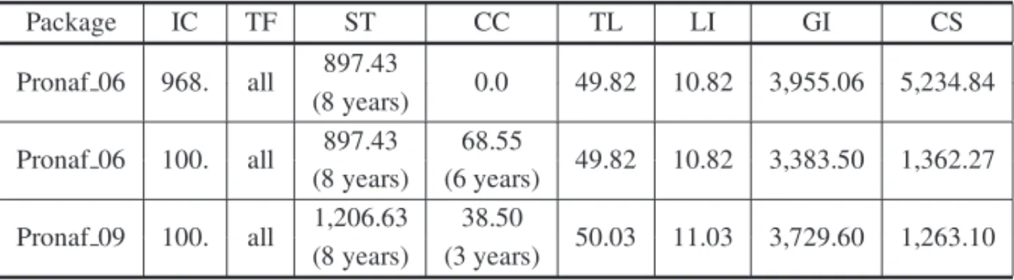
The results obtained from supposing there is 200 additional hours available of seasonal family labor in the months of intensive activities are shown in Table 4 and described as the following. As in the earlier section, the word “all”, below column TF in this table, represents the maximum acceptable value shown in Table 1. Information on planting area for each crop and need of hiring seasonal workers is presented in Tables 12, 13 and 14, Appendix 2.
Table 4– Production and financial results for farmers using bothPronaf financial packages and surplus family labor.
Package IC TF ST CC TL LI GI CS
Pronaf 06 968. all 897.43 0.0 49.82 10.82 3,955.06 5,234.84 (8 years)
Pronaf 06 100. all 897.43 68.55 49.82 10.82 3,383.50 1,362.27 (8 years) (6 years)
Pronaf 09 100. all 1,206.63 38.50 50.03 11.03 3,729.60 1,263.10 (8 years) (3 years)
If an initial capital contribution is 968 u.m. for investments in the year 2006 the farmer could take the whole loan amount from thePronaf long-term credit line and an annual average of 897.43 u.m. from the short-term credit line throughout the planning horizon. In this case, by annually using a land area of 49.82 ha for planting corn, soybeans and wheat in a rotation system, the gross farm income could present an annual average of 3,955.06 u.m. and the account balance of the farm could be closed with an amount of 5,234.84 u.m. at the end of the planning horizon.
If there is an initial capital contribution of just 100 u.m., the farmer could take the same amount of credit from thePronaf 06financial package in the earlier case. The results obtained indicate that by using a land area of 49.82 ha for annually planting rice, corn, soybeans and wheat crops, the farmer could get a gross farm income with an average of 3,383.5 u.m. a year and the account balance of the farm could be closed with 1,362.27 u.m. at the end of planning horizon. Also, he would have to take a monthly average of 68.55 u.m. from his credit card over the first six years for balancing the monthly accounts of the farm.
For all cases shown in both Tables 3 and 4, the user of credit fromPronaf 06and/orPronaf 09
could pay off his debts during the real planning horizon of eight years and five months.
4.2 Proger Financial Packages
This subsection presents results attained from running the new versions of the programs when applying theProgerfinancial packages described in 3.2. In Tables 5 and 6, below, the financial packages considered for the years 2006 and 2009 are denominatedProger 06andProger 09, respectively.
4.2.1 No surplus family labor
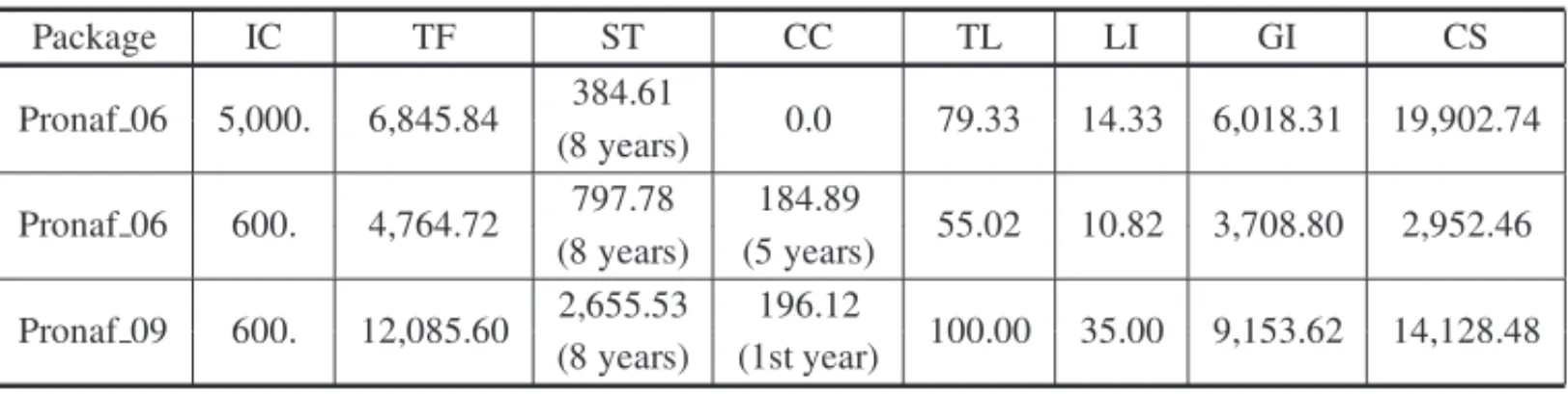
The results obtained by supposing there is no use of additional seasonal family labor in the months of intensive activities are depicted in Table 5 and described below. Detailed information on planting area for each crop and need of hiring seasonal workers is showed in Tables 15, 16 and 17, Appendix 2.
Table 5– Production and financial results for farmers usingProgerfinancial packages.
Package IC TF ST CC TL LI GI CS
Pronaf 06 5,000. 6,845.84 384.61 0.0 79.33 14.33 6,018.31 19,902.74 (8 years)
Pronaf 06 600. 4,764.72 797.78 184.89 55.02 10.82 3,708.80 2,952.46 (8 years) (5 years)
Pronaf 09 600. 12,085.60 2,655.53 196.12 100.00 35.00 9,153.62 14,128.48 (8 years) (1st year)
With an initial capital contribution of 5,000 u.m. in the year 2006, the obtained solution in-dicates that the user of credits from the Proger financial package could take the amount of 6,845.84 u.m. from bothProger RuralandModeragrocredit lines. Furthermore, an annual av-erage of 384.61 u.m. could be taken from theProger Custeioshort-term credit line throughout the entire planning horizon. In this way, the farmer could use 65 ha of land area in the first two years, and 79.33 ha from the third year for annually planting corn, soybeans and wheat in a rotation system to get an annual average of gross farm income of 6,018.31 u.m. and to close the account balance of the farm with 19,902.74 u.m. at the end of the planning horizon of eight years and five months.
would have to use a monthly average amount of 184.89 u.m. from his credit card over the first five years.
In the year 2009, if there is an initial capital contribution of 600 u.m., the user of Proger 09
could take the amount of 12,085.60 u.m. from theModeragroandProger Ruralcredit lines, and an annual average of 2,655.53 u.m. from theProger Custeiocredit line over the entire planning horizon. With this capital, the farmer could use 95.90 ha in the first year, and from the second year 100 ha of land to annually plant corn, soybeans, rice and wheat in a rotation system in order to obtain an annual gross farm income average of 9,153.62 u.m. and to close the account balance of the farm with the amount of 14,128.48 u.m. at the end of the planning horizon. For attaining these results, the farmer would have to take a monthly average of 196.12 u.m. from his credit card in the first year of the planning horizon.
4.2.2 With surplus family labor
The results obtained by supposing the use of additional seasonal family labor in the months of intensive activities are depicted in Table 6 below, and described as the following. Information about planting area for each crop and need of hiring seasonal workers is showed in Tables 18, 19 and 20, Appendix 2.
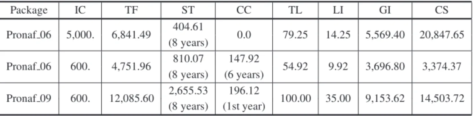
Table 6– Production and Financial results for farmers using bothProgerfinancial packages and surplus seasonal family labor.
Package IC TF ST CC TL LI GI CS
Pronaf 06 5,000. 6,841.49 404.61 0.0 79.25 14.25 5,569.40 20,847.65 (8 years)
Pronaf 06 600. 4,751.96 810.07 147.92 54.92 9.92 3,696.80 3,374.37 (8 years) (6 years)
Pronaf 09 600. 12,085.60 2,655.53 196.12 100.00 35.00 9,153.62 14,503.72 (8 years) (1st year)
With an initial capital contribution of 5,000 u.m., the user of credit from theProger 06financial package could take an amount of 6,841.49 u.m. from bothProger RuralandModeragrocredit lines, and an annual average of 404.61 u.m. from theProger Custeio short-term credit line throughout the entire planning horizon. In this way, he could use a land area of 65 ha in the first year, and 79.25 ha from the second year for annually planting corn, soybeans and wheat in a rotation system, to get an annual gross farm income average of 5,569.40 u.m., and to close the account balance of the farm with 20,847.65 u.m. at the end of the planning horizon.
average of 3,696.80 u.m. and finish the planning horizon with 3,374.37 u.m. in the account balance of the farm. For that, he would have to take money from his credit card during the first six years with a monthly average of 147.92 u.m.
In the year 2009, if there is an initial capital contribution of 600 u.m., the user ofProger 09
could obtain results that only differ to those displayed in Table 5 in the value of the final account balance surplus, which could be of 14,503.72 u.m. at the end of the planning horizon.
For all cases shown in both Tables 5 and 6, the user of credit fromProger 06and/orProger 09
could pay his debts over the real planning horizon of eight years and five months.
5 DISCUSSION
In order to include in this discussion results related to the year 2002, it is important to under-score some differences existing among the initial conditions of thePronaf andProgerprograms considered for that time and those ones considered in the present work.
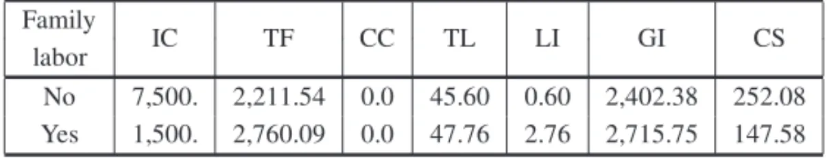
As the authors mentioned in their work (Biagio et al., 2007), in the year 2002 the long-term credit lines had the period for debt payments extended to ten years and five months due to sys-tem feasibility purposes. Furthermore, parameters like the amount of money monthly set aside for the family’s consumption, costs with seasonal labor and interest rates are upgraded for all implemented programs in the present study. The first two parameters are strongly related to the Brazilian minimum wage, so their values have changed as described in subsection 3.3 above (see Appendix 1 for the year 2002) and below:
• for thePronafprograms, the parameter related to the family’s consumption was considered to be 16.65% and 37.66%, respectively in the years 2006 and 2009, larger than that in the year 2002;
• for theProgerprograms, respectively in the years 2006 and 2009, the family’s consump-tion parameter was 16.65% and of 55.00% larger than the one in the year 2002;
• in the year 2009, and for both programs, seasonal labor costs were considered to be 41.66% larger than the one in the years 2002 and 2006.
By taking into account the differences cited above, it is possible to observe from the results shown in both Tables 3 and 4, subsection 4.1, and Table 7 in the Appendix 1, for the user of
Pronaf financial packages:
(i) In the year 2002, if the initial capital contribution is 1,500 u.m. and additional seasonal family labor is being used, it would be necessary to take the total loan from thePronaf
(ii) Different from the situation in the year 2002, the farmer who took money fromPronaf in the years 2006 and/or 2009, could pay his debts over a planning horizon of eight years and five months. Furthermore,
– in the year 2006, the user ofPronaf 06could take a larger loan amount and invest a smaller initial capital contribution amount than those in the year 2002; also, in all scenarios shown the farmer could achieve a good gross income and surplus in the account balance of the farm at the end of the planning horizon. If investing just 100 u.m. of an initial capital contribution, the farmer would have to use his credit card monthly over five or six years depending on the use of seasonal family labor;
– in the year 2009, with a larger loan amount from the short-term credit line, the Pronaf 09 user could initially invest a small amount of his/her capital contribution of 100 u.m. and attain better production and financial results along the planning hori-zon than those obtained fromPronaf 06. Moreover, given that 50.03 ha of land could be used for planting, the annual farm income average could increase and the average amount of money taken monthly from the credit card decreases.
From the results shown in both Tables 5 and 6, subsection 4.2, and Table 8 in the Appendix 1, it is possible to see that for the user ofProgerfinancial packages:
(i) In the year 2002, if investing 5,000 u.m. of initial capital, the user of theProger 02package could achieve good production and gross farm income, with exception to the final account balance surplus; if investing just 100 u.m. of a capital contribution, the farmer must use surplus seasonal family labor and his credit card in order to get feasible financial results from the production system;
(ii) Different from the situation in the year 2002, the farmer who took money fromProger
in the years 2006 and/or 2009, could pay off his debts during a planning horizon of eight years and five months. Besides this,
– with an amount of 5,000 u.m. of an initial capital contribution in the year 2006, the
Proger 06package user could get much better results than in the year 2002 since he could take out a larger loan amount and consequently, attain increases in both annual average farm income and final account balance surplus;
– if investing 600 u.m. of an initial capital contribution, the user ofProger 06could take a somewhat bigger loan than in the second scenario of the year 2002 and ob-tain financial feasibility for the production system by planting in a reduced area of land, using a larger credit card amount and sustaining decreased values of gross farm income and final account balance surplus;
In relation to the financial benefits of seasonal family labor participation in the production sys-tems, it can be observed from the results shown in Tables 3 to 8 that:
• When applying Pronaf 02in the year 2002 (see Appendix 1), the farmer could obtain an increase in the annual average of gross farm income with a decreased amount of ini-tial capital contribution. For the user of theProger 02package, production and financial feasibility of the system could be obtained from a small initial capital contribution;
• In the year 2006, the farmer who took money from thePronaf 06package could obtain a little larger account balance surplus than that one obtained with no surplus seasonal family labor. For the user of theProger 06package, it could be possible to attain a slight increase in the final account balance surplus and a decrease in the monthly loan average taken from the credit card when using a small amount of initial capital contribution;
• In the year 2009, the user ofPronaf 09could obtain some financial system improvements, given the modest increase in the values of both the annual average of gross farm income and the final account balance surplus. For the user of theProger 09package, the finan-cial results shown did not indicate significant improvements in any case, given only the relatively small increase attained in the value of the final account balance surplus.
With respect to the bank requirements on annual average of gross farm income mentioned in subsections 3.1 and 3.2, some additional observations on economic and financial feasibility im-provements of farm systems during the last decade can also be made based on the results shown in the last section:
• All cases related to the use of loans fromPronaf 06andPronaf 09present possible solu-tions for the production system, which also satisfy the financial bank constraints;
• For medium farmers, despite the favorable solutions provided byProger 06, the annual average of gross farm income could not satisfy the upper bound established by the banks when investing an initial capital contribution of 5,000 u.m. and planting in a larger land area;
• TheProger 09financial package considered in this work could guarantee financial solu-tions for the production systems in accordance to bank criteria.
6 CONCLUSIONS
In this paper, new versions of mathematical programs for crop production planning problems in farm systems with up to 100 ha of land area were implemented and several scenarios were successfully run. They generated solutions from which it is possible to affirm that:
• Differently from the financial packages considered in the year 2002, both Pronaf and
• For small systems, besides the increased amounts of credit, in the years 2006 and 2009, good results were possible to observe when the farmer having some amount of an initial capital contribution for investments and, additionally, using a credit card to balance the monthly accounts of the farm, independent of using additional seasonal family labor;
• The increased amount of credits available for medium farmers, in the year 2009, could provide the agricultural systems with better solutions than those obtained for the years 2002 and 2006. Also, the limits on gross farm income established by financial institutions improved the feasibility between production and bank constraints;
• For all systems tested in this study, the results obtained showed that the financial im-portance of surplus seasonal family labor decreased during the last decade and could be substituted by seasonal workers.
For the Brazilian agricultural sector, these are favorable results since they indicate production and financial improvements for small systems during the last decade, which are also accomplished by the socio-economic improvements given by the feasibility of hiring seasonal workers.
REFERENCES
[1] BIAGIOMA, ABE EN, TURNES O. 2007. Modelo para planejamento gerencial de produc¸˜ao em fazenda familiar no cerrado brasileiro.Pesquisa Operacional,27(3): 377–405.
[2] DALTONGE. 1982. Managing agricultural systems. London:Applied Science Publishers.
[3] DENT JB. 1990. Optimising the mixture of enterprises in a farming system. In: Systems Theory Applied to Agriculture and the Food Chain[edited by JONESJGW & STREETPR], London, Elsevier Applied Science, p. 113–130.
[4] DENTJB, HARRISONSR & WOODFORDKB. 1986. Farm planning with linear programming: con-cept and practice, Sidney: Butterworths.
[5] GUANZIROLICE. 2007. PRONAF dez anos depois: resultados e perspectivas para o desenvolvi-mento rural.Rev. Econ. Sociol. Rural,27: 301–328.
[6] IBGE, CENSO AGROPECUARIO´ 2006: Brasil, grandes regi˜oes e unidades da federac¸˜ao (//www.ibge.gov.br/home/estatistica/economia/agropecuaria/censoagro/).
[7] VELOSORF. 1990. Crop farm development in the Brazilian Cerrado region: an ex-ante evaluation. PhD.Thesis, University of Edinburgh.
[8] VELOSORF, CARVALHOERO & GOULARTAM. 1997. Economic and financial performance eval-uation of a farm in the Brazilian savannas. In: Applications of systems approaches at the farm and regional levels[edited by TENGPS, KROPFFMJ,TENBERGEHFM, DENTJB, LANSIGANFP &
VANLAARHH], Kluwer Academic Publications, v.1.
A APPENDIX 1
This appendix summarizes, in the subsections below, a description of thePronaf andProger
following matrix dimensions: 1758 constraints and 2722 variables when applyingPronaf, and 1677 constraints and 2508 variables when applyingProger.
By using the notations defined in section 4, Tables 7 and 8 below, depict results that were attained for an extended planning horizon of ten years and five months. For these results, the parameters related to a family’s consumption and costs with seasonal labor were assumed to be equal to 57.69 u.m. and 0.12 u.m. an hour, respectively, for bothPronafandProgerpackages.
A.1 PronafPackage
In the year 2002, thePronaffinancial package was composed of the long-termPronaf D,Pronaf Agregar andProger Rural Tradicional credit lines, the last one being a long-term credit line with a high annual interest rate of 19,25% (known asProger withTJLP). ThePronaf D and
Pronaf Agregar were proposed to help farm infrastructure improvements, including acquiring irrigation systems and machinery. Each of these credit lines had an annual interest rate of 4% and, for feasibility purposes it was supposed that each of them allowed credit amounts of 1,105.77 u.m. which were 15% larger than the real ones. In this year, thePronafpackage did not offer a short-term credit line and the farmer had no available credit card. The results are shown in Table 7 below.
Table 7– Financial and production results for users ofPronaffinancial packages.
Family
IC TF CC TL LI GI CS
labor
No 7,500. 2,211.54 0.0 45.60 0.60 2,402.38 252.08 Yes 1,500. 2,760.09 0.0 47.76 2.76 2,715.75 147.58
As it is depicted in the table above, without using additional seasonal family labor, it was nec-essary for thePronaf user to have an initial capital contribution of 7,500.00 u.m. and to take an amount of 2,211.54 u.m. from the credit lines in order to obtain production system feasibil-ity. Furthermore, for attaining the results, the farmer must take 408.23 u.m. from a hypothetical short-term credit line in the 10th year.
If using 200 additional hours of seasonal family labor, an initial capital contribution of 1,500.00 u.m. was required by the farmer in order for the production system to be feasible. Besides this, the farmer needs to take an amount of 2,760.09 u.m. from thePronaf credit line and part of the credit allowed byProgerwithTJLPin the first year. In addition, the farmer must take an annual average of 247,52 u.m. from a hypothetical short-term credit line over the first seven years, paying an interest rate of 15,25% a year.
A.2 ProgerPackage
TheProger financial package considered for the year 2002 was composed of three long-term credit lines and one short-term. The long-term were the following:Modefrota, Prosolo and
and third credit lines for soil input expenses and investments in irrigation systems, respectively. An interest rate of 8.5% a year was pre-determined for each of these credit lines.
TheFCO(Brazilian Constitutional Funds for the Mid-West Region) short-term credit line con-sidered allowed an amount of up to 3,205.13 u.m. with an interest rate of 8.5% a year. The
FCOcredit line also offered a discount of 15% on the interest rate for users with no overdue debt payments. There was an 8,3% monthly credit card interest rate in the year 2002. The results are shown in the table below.
Table 8– Financial and production results for users ofProgerfinancial package.
Family
IC TF CC TL LI GI CS
labor
No 5,000. 5,431.44 0.0 73.90 8.90 4,679.29 513.49 Yes 100. 4,483.34 78.46 65.26 8.90 3,958.14 1,773.67
Without using additional seasonal family labor as depicted in Table 8, the user of theProger
financial package must have an initial capital contribution of 5,000.00 u.m. and needs financing in the first year of 5,431.44 u.m. from bothProgerandProsolocredit lines for obtaining pro-duction system feasibility. For the results attained, the farmer also needs to take money from the short-term FCO credit line every year with an annual average of 1,602.56 u.m..
By using 200 hours of surplus seasonal family labor, and an initial capital contribution of 100 u.m., the farmer could take the amount of 4,483.34 from bothProger andProsolocredit lines in the first year. In order to obtain the results, the farmer needs to use a monthly average of 78.46 u.m. from his credit card in the first six years and take an annual average amount of 1,602.57 u.m. from the FCO short-term credit line along the extended planning horizon.
B APPENDIX 2
This appendix presents, in the tables from 9 to 20, the optimal solutions on crop planting areas and contracted man-hours, which are related to the scenarios depicted in tables from 3 to 6, Section 4.
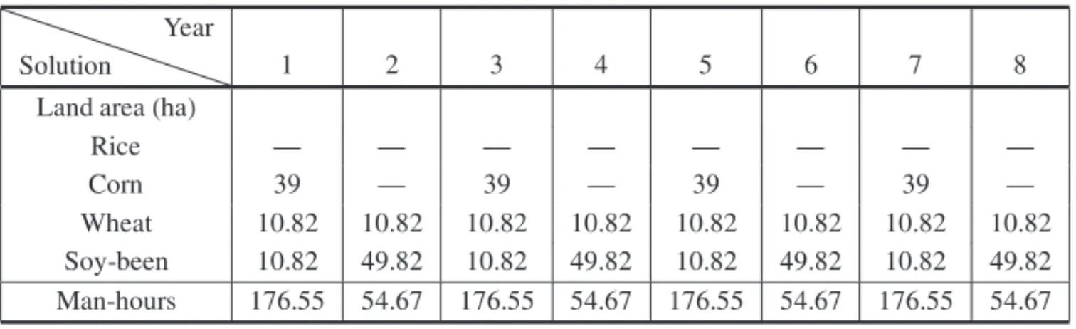
Table 9– Pronaf 06, without seasonal family labor, IC=968.00 u.m. and family’s consumption of 67.31 u.m. (CPU=0.19 sec.).
Solution Year
1 2 3 4 5 6 7 8
Land area (ha)
Rice — — — — — — — —
Corn 39 — 39 — 39 — 39 —
Table 10– Pronaf 06, without seasonal family labor, IC=100.00 u.m. and family’s consump-tion of 67.31 u.m. (CPU=0.30 sec.).
Solution Year
1 2 3 4 5 6 7 8
Land area (ha)
Rice — 39 — 39 — 15.26 — —
Corn — — — — — 23.74 — 39
Wheat 10.82 10.82 10.82 10.82 10.82 10.82 10.82 10.82 Soy-been 49.82 10.82 49.82 10.82 49.82 10.82 49.82 10.82 Man-hours 49.80 59.55 49.80 59.55 49.80 129.78 52.77 181.32
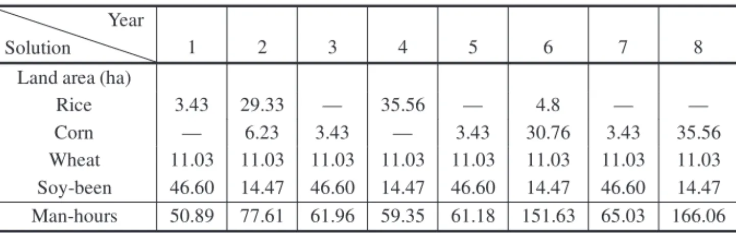
Table 11– Pronaf 09, without seasonal family labor, IC=100.00 u.m. and family’s consump-tion of 79.42 u.m. (CPU=0.34 sec.).
Solution Year
1 2 3 4 5 6 7 8
Land area (ha)
Rice 3.43 29.33 — 35.56 — 4.8 — —
Corn — 6.23 3.43 — 3.43 30.76 3.43 35.56 Wheat 11.03 11.03 11.03 11.03 11.03 11.03 11.03 11.03 Soy-been 46.60 14.47 46.60 14.47 46.60 14.47 46.60 14.47 Man-hours 50.89 77.61 61.96 59.35 61.18 151.63 65.03 166.06
Table 12– Pronaf 06, with seasonal family labor, IC=968.00 u.m. and family’s consump-tion of 67.31 u.m. (CPU=0.14 sec.).
Solution Year
1 2 3 4 5 6 7 8
Land area (ha)
Rice — — — — — — — —
Corn 39 — 39 — 39 — 39 —
Wheat 10.82 10.82 10.82 10.82 10.82 10.82 10.82 10.82 Soy-been 10.82 49.82 10.82 49.82 10.82 49.82 10.82 49.82
Man-hours 0. 0. 0. 0. 0. 0. 0. 0.
Table 13– Pronaf 06, with seasonal family labor, IC=100.00 u.m. and family’s consump-tion of 67.31 u.m. (CPU=0.16 sec.).
Solution Year
1 2 3 4 5 6 7 8
Land area (ha)
Rice — 39 — 39 — 11.71 — —
Corn — — — — — 27.29 — 39
Wheat 10.82 10.82 10.82 10.82 10.82 10.82 10.82 10.82 Soy-been 49.82 10.82 49.82 10.82 49.82 10.82 49.82 10.82
Table 14– Pronaf 09, with seasonal family labor, IC=100.00 u.m. and family’s consump-tion of 79.42 u.m. (CPU=0.34 sec.).
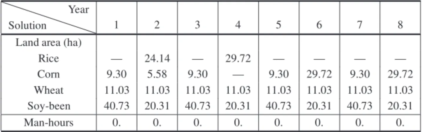
Solution Year
1 2 3 4 5 6 7 8
Land area (ha)
Rice — 24.14 — 29.72 — — — —
Corn 9.30 5.58 9.30 — 9.30 29.72 9.30 29.72 Wheat 11.03 11.03 11.03 11.03 11.03 11.03 11.03 11.03 Soy-been 40.73 20.31 40.73 20.31 40.73 20.31 40.73 20.31
Man-hours 0. 0. 0. 0. 0. 0. 0. 0.
Table 15– Proger 06, without seasonal family labor, IC=5,000.00 u.m. and family’s consump-tion of 67.31 u.m. (CPU=0.16 sec.).
Solution Year
1 2 3 4 5 6 7 8
Land area (ha)
Rice — — — — — — — —
Corn 65 — 65 — 65 — 65 —
Wheat — 14.33 14.33 14.33 14.33 14.33 14.33 14.33 Soy-been — 65 14.33 79.33 14.33 79.33 14.33 79.33 Man-hours 276.25 87.44 290.57 87.44 290.57 87.44 290.57 87.44
Table 16– Proger 06, without seasonal family labor, IC=600.00 u.m. and family’s consump-tion of 67.31 u.m. (CPU=0.19 sec.).
Solution Year
1 2 3 4 5 6 7 8
Land area (ha)
Rice 6.49 32.68 — 38.51 6.49 — — —
Corn — 5.83 6.49 — — 38.51 6.49 38.51
Wheat — 10.02 10.02 10.02 10.02 10.02 10.02 10.02 Soy-been 38.51 16.51 48.53 16.51 48.53 16.51 48.53 16.51 Man-hours 46.61 82.14 76.80 65.44 56.61 180.19 80.89 181.00
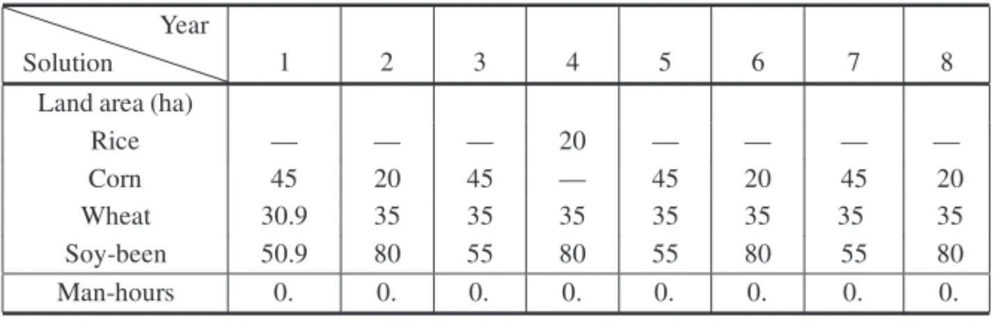
Table 17– Proger 09, without seasonal family labor, IC=600.00 u.m. and family’s consumption of 89.42 u.m. (CPU=0.17 sec.).
Solution Year
1 2 3 4 5 6 7 8
Land area (ha)
Rice — — — 20 — — — —
Corn 45 20 45 - 45 20 45 20
Wheat 30.9 35 35 35 35 35 35 35
Soy-been 50.9 80 55 80 55 80 55 80
Table 18– Proger 06, with seasonal family labor, IC=5,000.00 u.m. and family’s consump-tion of 67.31 u.m. (CPU=0.24 sec.).
Solution Year
1 2 3 4 5 6 7 8
Land area (ha)
Rice — — — — — — — —
Corn 65 — 65 — 65 — 65 —
Wheat — 14.25 14.25 14.25 14.25 14.25 14.25 14.25 Soy-been — 79.25 14.25 79.25 14.25 79.25 14.25 79.25 Man-hours 27.5 0. 31.06. 0. 31.06. 0. 31.06. 0.
Table 19– Proger 06, with seasonal family labor, IC=600.00 u.m. and family’s consump-tion of 67.31 u.m. (CPU=0.19 sec.).
Solution Year
1 2 3 4 5 6 7 8
Land area (ha)
Rice 5.40 31.98 — 38.53 6.47 — — —
Corn 1.07 6.55 6.47 — — 38.53 6.47 38.53 Wheat — 9.92 9.92 9.92 9.92 9.92 9.92 9.92 Soy-been 38.53 16.39 48.45 16.39 48.45 16.39 48.45 16.39
Man-hours 0. 0. 0. 0. 0. 0. 0. 0.
Table 20– Proger 06, with seasonal family labor, IC=600.00 u.m. and family’s consump-tion of 89.42 u.m. (CPU=0.19 sec.).
Solution Year
1 2 3 4 5 6 7 8
Land area (ha)
Rice — — — 20 — — — —
Corn 45 20 45 — 45 20 45 20
Wheat 30.9 35 35 35 35 35 35 35
Soy-been 50.9 80 55 80 55 80 55 80