Statistical Approaches Concerning the Relationship between the Health Index and the Life Expectancy, in Romania

(1)

Annals of “Dunarea de Jos” University of Galati Fascicle I. Economics and Applied Informatics

Years XXI – no_2/2015 ISSN-L 1584-0409 ISSN-Online 2344-441X

www.eia.feaa.ugal.ro

Statistical Approaches Concerning the Relationship

between the Health Index and the Life Expectancy, in

Romania

Gabriela OPAIT

A R T I C L E I N F O A B S T R A C T

Article history:

Accepted May

Available online August

JEL Classification

C , C , C

Keywords:

(ealth )ndex, Life Expectancy, Correlation Raport, T test

This research reflects the methodology for to achieve the statistical modeling of the trend concerning the correlation between the (ealth )ndex and the Life Expectancy in Romania, in the period - . with the help of the „Least Squares Method , which is a method through we can to express the trend line of the best fit concerning a model. Also, this paper reflects the manner in which we can to measure the intensity regarding the correlation between the (ealth )ndex and the Life Expectancy in Romania, between - with the help of the Correlation Raport and how we can to reflect that there is a significant diferrence between the values of the (ealth )ndex in Romania and the values of the (ealth )ndex in U.S.A., respectively the values of the (ealth )ndex in Norway by means of the T test.

1. Introduction

)n this paper, ) present a personal contribution which reflects a statistical analysis of the trend model between the (ealth )ndex and the Life Expectancy in Romania, in the period - . The purpose of the research reflects the possibility for to reflect the intensity of the correlation with the help of the Correlation Raport. The statistical methods used are the „Coefficients of Variation Method , respectively the „Least Squares Method applied for to calculate the parameters of the regression equation and the Method of the Correlation Raport used for to reflect the intensity of the correlation between the (ealth )ndex and the Life Expectancy. The sections presents the methodology for to achieve the trend model between the (ealth )ndex and the Life Expectancy in Romania, in the period - , with the help of the „Least Squares

Method . The section reflects the intensity of the correlation between the (ealth )ndex and the Life

Expectancy in Romania, between - . The section reflects how we apply the t test for to express if

there is a significant diference between the (ealth )ndex in Romania and the (ealth )ndex in U.S.A respectively the (ealth )ndex in Norway, in the period - . The state of the art in this domain is represented by the research belongs to Carl Friederich Gauss, who created the „Least Squares Method[ ].

2. The modeling of the trend between the Health Index and the Life Expectancy in Romania, between 2005-2014

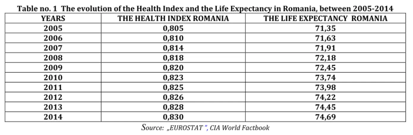
)n the period - , we observe the next evolution concerning the (ealth )ndex and the Life Expectancy in Romania, according to the table no. :

Table no. 1 The evolution of the Health Index and the Life Expectancy in Romania, between 2005-2014

YEARS THE HEALTH INDEX ROMANIA THE LIFE EXPECTANCY ROMANIA

2005 0,805 71,35

2006 0,810 71,63

2007 0,814 71,91

2008 0,818 72,18

2009 0,820 72,45

2010 0,823 73,74

2011 0,825 73,98

2012 0,826 74,22

2013 0,828 74,45

2014 0,830 74,69

Source: „EUROSTAT ”, CIA World Factbook

(2)

We want to identify the trend model between the (ealth )ndex and the Life Expectancy for Romania, in the period - , using the table no. .

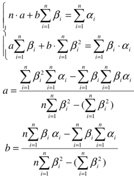
- if we formulate the null hypothesis

H

0: which mentions the assumption of the existence for the model of tendency concerning

α

factor, where

α

= the Life Expectancy in Romania, as being the function

i ti

a

b

β

α

=

+

⋅

, then the parameters a and b of the adjusted linear function, can to be calculated by means of

the next system [ ]:

⎪

⎩

⎪⎪

⎨

⎧

⋅

=

⋅

+

=

+

⋅

∑

= =

=

= =

n

i

i i n

i i

n

i i n

i i

b

a

b

a

n

1 1

2

1

1 1

α

β

α

β

Therefore,

∑

= =

= = =

=

−

=

_n

i i n

i i

i n

i i n

i i

n

a

1 2

1 1 1

1 2

)

(

β

α

β

α

β

∑

= =

= = =

−

=

_n

i i n

i i

n

i i n

i i i

n

b

1 2

1 1 1

)

(

β

α

β

α

β

Table no. 2 The estimate of the value for the variation coefficient in the case of the adjusted linear function, in the hypothesis concerning the linear evolution of the

correlation between the Health Index in Romania and the Life Expectancy in Romania, between 2005-2014

LINEAR TREND

YEARS

THE HEALTH

INDEX Romania

(

β

i)

THE LIFE EXPECTANCY

Romania

(

α

i)

2

i

β

_i

α

_i

i

b

a

i

β

α

_β

=

+

i

α

β

α

−

2005 0,805 71,35 , , , ,

2006 0,810 71,63 , , , ,

2007 0,814 71,91 , , , ,

2008 0,818 72,18 , , , ,

2009 0,820 72,45 , , , ,

2010 0,823 73,74 , , , ,

2011 0,825 73,98 , , , ,

2012 0,826 74,22 , , , ,

2013 0,828 74,45 , , , ,

2014 0,830 74,69 , , , ,

TOTAL 8,199 730,6 , , , ,

)f we calculate the statistical data for to adjust the linear function, we obtain for the parameters a and b the

values:

49 ,

64434797

)

199 ,

8 (

722959

,

6

10 10857

,

599

199 ,

8

6 ,

730 722959

,

6

2

=

−

⋅

−

⋅

=

a

149 ,

6577058

)

199 ,

8 (

722959

,

6

10

6 ,

730

199 ,

8 10857

,

599

10

2

=

−

⋅

−

⋅

=

(3)

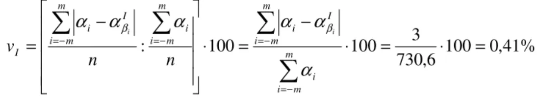
(ence, the coefficient of variation for the adjusted linear function is:

%

41 ,

0

100

6 ,

730

3

100

100 :

⋅

=

⋅

=

−

=

⋅

⎥

⎦

⎤

⎢

⎣

⎡

−

=

∑

− = − = − = − = m m i i m m i I i m m i i m m i I i I i i

n

v

α

β β

- in the situation of the alternative hypothesis

H

1 : which specifies the assumption of the existence for the model of tendency regarding

α

factor, where

α

= the Life Expectancy, as being the quadratic function

2

i i

c

b

a

i

β

α

_β

=

+

⋅

+

, the parameters a, b şi c of the adjusted quadratic function, can to be calculated by

means of the system [ ]:

∑

= =

=

−

=

⇔

=

−

=

n i i i i n i i

i

S

a

b

c

S

1 2 2 1 2

min

)

(

min

)

(

α

_β

α

β

⇒

⎪

⎩

⎪

⎨

⎧

=

∂

=

∂

=

∂

0

0 c

S

b

S

a

S

⇒

⎪

⎩

⎪⎪

⎪

⎨

⎧

−

=

−

=

−

=

−

∑

= =

)

2

1 /(

0 )

)(

(

2 )

2

1 /(

0 )

)(

(

2 )

2

1 /(

0 )

1 )(

(

2

2 2 1 1 2 1 1 2 i i i i n i i i i n i i i

c

b

a

c

b

a

c

b

a

β

α

β

α

β

α

Therefore,

⎪

⎩

⎪

⎨

⎧

⋅

=

+

⋅

=

+

⋅

+

=

+

⋅

∑

= = = = = = = = = = = n i i i n i i n i i n i i n i i i n i i n i i n i i n i i n i i n i i

c

b

a

c

b

a

c

b

a

n

1 2 1 4 1 3 1 2 1 1 3 1 2 1 1 1 2 1

α

β

α

β

α

β

Table no. 3 The estimates of the value for the variation coefficient in the case of the adjusted quadratic function, in the hypothesis concerning the parabolic evolution of the correlation between

the Health Index and the Life Expectancy in Romania, between 2005-2014 PARABOLIC TREND YEARS THE HEALTH INDEX Romania

(

β

i)

LIFE EXPEC-TANCY

Roma nia

(

α

i)

3

i

β

4

i

β

i

α

i

2 2 i i

c

b

a

i

β

α

β

=

+

i

α

β

α

−

2005 0,805 71,35 , , , , ,

2006 0,810 71,63 , , , , ,

2007 0,814 71,91 , , , , ,

2008 0,818 72,18 , , , , ,

2009 0,820 72,45 , , , , ,

2010 0,823 73,74 , , , , ,

2011 0,825 73,98 , , , , ,

2012 0,826 74,22 , , , , ,

2013 0,828 74,45 , , , , ,

2014 0,830 74,69 , , , , ,

(4)

)f we calculate the statistical data for to adjust the quadratic function, we obtain for the parameters a,b and c

the next values:

⇒

⎪

⎩

⎪

⎨

⎧

=

⋅

+

⋅

+

⋅

=

⋅

+

⋅

+

⋅

=

⋅

+

⋅

+

⋅

3261279

,

491 521419891

,

4 513133621

,

5 722959

,

6 10857

,

599 513133621

,

5 722959

,

6

199 ,

8

6 ,

730 722959

,

6

199 ,

8

10 c

b

a

c

b

a

c

b

a

=

3485

,

796077

b

=

−

8500

,

623978

c

=

5290

,

714286

So, the coefficient of variation for the adjusted quadratic function has the value:

%

27 ,

0

100

6 ,

730

95 ,

1

100

100 :

⋅

=

⋅

=

−

=

⋅

⎥

⎦

⎤

⎢

⎣

⎡

−

=

∑

− = − = − = − = m m i i m m i II i m m i i m m i II i II i i

n

v

α

β β

- in the case of the alternative hypothesis

H

₂ : which describes the supposition the assumption of the

existence for the model of tendency concerning

α

factor, where

α

= the Life Expectancy in Romania,as

being the exponential function i i

ab

β β

α

=

, then the parameters a and b of the adjusted exponential function,

can to be calculated by means of the next system [ ]:

∑

= =

=

−

=

⇔

=

−

=

n i i i n i

i

S

a

b

S

i 1 2 1 2

min

)

lg

(lg

min

)

lg

(lg

α

_ξ

α

β

⇒

⎪

⎩

⎪⎪

⎨

⎧

=

∂

=

∂

0 lg

b

S

a

S

⇒

⎪

⎩

⎪⎪

⎨

⎧

−

=

−

=

−

∑

= = n i i i n i i

b

a

b

a

1 1 1 1

)

2

1 /(

0 )

)(

lg

(lg

2 )

2

1 /(

0 )

1 )(

lg

(lg

2 β

β

α

β

α

⎪

⎩

⎪⎪

⎨

⎧

⋅

=

⋅

+

=

⋅

+

⋅

∑

= = = = = n i i i n i i n i i n i i n i i

b

a

b

a

n

1 1 2 1 1 1

lg

α

β

α

β

Thus,

∑

= = = = = = = = = = = = = ⎟ ⎠ ⎞ ⎜ ⎝ ⎛ − − = = n i n i i i n i i n i i n i i i n i i i n i i n i i n i i n i n i i i n i i n i i n n a i 1 2 1 2

1 1 1 1

(5)

∑

= =

= = =

= =

= = =

=

⎟ ⎠ ⎞ ⎜ ⎝ ⎛

− − ⋅

= =

n i

i i

n

i i

n i

i n

i i i

i

n i

i n

i i

n i

i n i

i n

i i

n i

i

n n

b

i

1

2

1 2

1 1 1

1 2

1

1 1 1

1

lg lg

lg

β

α

β

α

β

α

Table no. 4 The estimate of the value for the variation coefficient in the case of the adjusted exponential function, in the hypothesis concerning the exponential evolution of the correlation between the Health Index in Romania and the Life Expectancy in Romania,

between 2005-2014

EXPONENTIAL TREND

YEARS

THE HEALTH

INDEX Roma nia (

β

_i)

THE LIFE EXPEC TANCY Roma nia

(

α

_i)

lg

α

i

β

i

lg

α

i

α

βi

=

lg

b a _ilg

lg +

β

=

i

ab

i

β β

α

=

α

i

−

α

βi

2005 0,805 71,35 , , , , ,

2006 0,810 71,63 , , , , ,

2007 0,814 71,91 , , , , ,

2008 0,818 72,18 , , , , ,

2009 0,820 72,45 , , , , ,

2010 0,823 73,74 , , , , ,

2011 0,825 73,98 , , , , ,

2012 0,826 74,22 , , , , ,

2013 0,828 74,45 , , , , ,

2014 0,830 74,69 , , , , ,

TOTAL 8,199 730,6 , , ,

Consequently, if we calculate the statistical data for to adjust the exponential function, we obtain for the parameters a and b the values:

132960427 ,

1

722959 , 6 199 , 8

199 , 8 10

722959 , 6 28035315 ,

15

199 , 8 63619885 ,

18

lga= =

₀_,_891150442

722959 , 6 199 , 8

199 , 8 10

28035315 ,

15 199 , 8

63619885 ,

18 10

lgb= =

Accordingly, the coefficient of variation for the adjusted exponential function has the next value:

%

40 ,

0

100

6 ,

730

94 ,

2

100

100 :

exp exp

exp

⋅

=

⋅

=

−

=

⋅

⎥

⎦

⎤

⎢

⎣

⎡

−

=

∑

− = − = −

= −

=

m

m i

i m

m i

i m

m i

i m

m i

i _i _i

n

v

α

_β _β

We apply the coefficients of variation method as criterion of selection for the best model of trend.

(6)

%

40 ,

0 %

41 ,

0 %

27 ,

0 <

=

<

_exp

=

v

II I

So, the path reflected by the correlation between the Life Expectancy in Romania and the Health Index in Romania, between 2005-2014, is a parabolical trend of the shape

α

β_i

=

a

+

b

⋅

β

i

+

c

β

i2, with other

words it confirms the hypothesis

H

1 .

71

0,8 0,85

PARABOLICAL TREND

The type no. 1 The trend model of the values for the correlation between the Life Expectancy and the Health Index in Romania, in the period 2005-2014

We observe that, the cloud of points which reflects the values of the the Life Expectancy in Romania in function of the (ealth )ndex in Romania, between - , it carrying around a parabolical model of trend, according to the type no. .

3. The intensity of the correlation between the Health Index in Romania and the Life Expectancy in Romania, in the period 2005-2014.

For to reflect the intensity of the parabolical correlation between the (ealth )ndex in Romania and theLife Expectancy in Romania, in the period - , we use the Correlation Raport noted with

η

[ ]:

n

c

b

a

n

i i n

i i

n

i i n

i

i i n

i i i n

i i

⎟

⎠

⎞

⎜

⎝

⎛

−

⎟

⎠

⎞

⎜

⎝

⎛

−

+

=

∑

=

= =

=

1 2

2

1

1 2

1 1

α

β

α

β

(7)

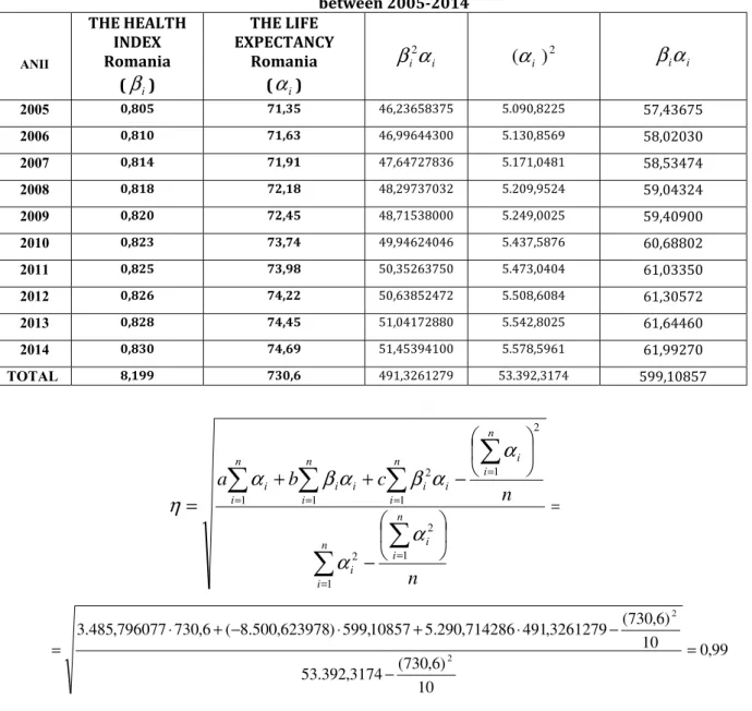
Table no. 5 The calculation of the value for the Correlation Raport in the case of the parabolical correlation between the Health Index and the Life Expectancy in Romania,

between 2005-2014

ANII

THE HEALTH INDEX Romania

(

β

_i)

THE LIFE EXPECTANCY

Romania (

α

_i)

i i

α

β

2

₍

₎

2

i

α

β

i

α

i

2005 0,805 71,35 , . , ,

2006 0,810 71,63 , . , ,

2007 0,814 71,91 , . , ,

2008 0,818 72,18 , . , ,

2009 0,820 72,45 , . , ,

2010 0,823 73,74 , . , ,

2011 0,825 73,98 , . , ,

2012 0,826 74,22 , . , ,

2013 0,828 74,45 , . , ,

2014 0,830 74,69 , . , ,

TOTAL 8,199 730,6 , . , ,

n

c

b

a

n

i i n

i i

n

i i n

i

i i n

i i i n

i i

⎟

⎠

⎞

⎜

⎝

⎛

−

⎟

⎠

⎞

⎜

⎝

⎛

−

+

=

∑

=

= =

=

1 2

2

1

1 2

1 1

α

β

α

β

α

η

=

99 , 0 10

) 6 , 730 ( 3174 , 392 . 53

10 ) 6 , 730 ( 3261279 ,

491 714286 , 290 . 5 10857 , 599 ) 623978 , 500 . 8 ( 6 , 730 796077 , 485 . 3

2

= −

− ⋅

+ ⋅

− + ⋅ =

)n conclusion, because the value of the Correlation Raport tends to , there is a very strong intensity between the (ealth )ndex in Romania and the Life Expectancy in Romania, between - .

4. The reflection of the methodology for to apply the T test.

According to the table no. , we observe between - , the next evolution concerning the (ealth )ndex in U.S.A which is on the third place in the world regarding the (ealth )ndex.

Table no. 6 The evolution of the Health Index in U.S.A., between 2005-2014

YEARS THE HEALTH INDEX (U.S.A.)

2005 0,887 2006 0,890 2007 0,892 2008 0,895 2009 0,898 2010 0,900 2011 0,902 2012 0,905 2013 0,907 2014 0,909

(8)

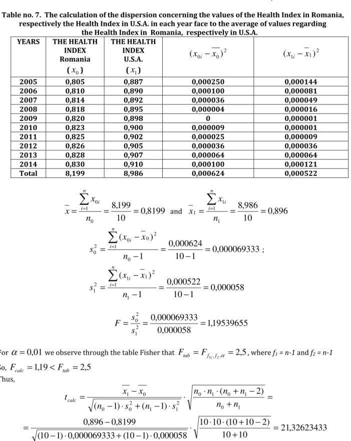
Through the help of the T test and F test, we want to know if there is a significant diference between the values of the (ealth )ndex in U.S.A. and and the values of the (ealth )ndex in Romania, between - .

Table no. 7. The calculation of the dispersion concerning the values of the Health Index in Romania, respectively the Health Index in U.S.A. in each year face to the average of values regarding the Health Index in Romania, respectively in U.S.A.

YEARS THE HEALTH INDEX Romania

(

x

₀)

THE HEALTH INDEX

U.S.A. (

x

₁)

2 0

0

)

(

x

_i

−

x

2

1

)

(

x

_i

−

x

2005 0,805 0,887 0,000250 0,000144

2006 0,810 0,890 0,000100 0,000081

2007 0,814 0,892 0,000036 0,000049

2008 0,818 0,895 0,000004 0,000016

2009 0,820 0,898 0 0,000001

2010 0,823 0,900 0,000009 0,000001

2011 0,825 0,902 0,000025 0,000009

2012 0,826 0,905 0,000036 0,000036

2013 0,828 0,907 0,000064 0,000064

2014 0,830 0,910 0,000100 0,000121

Total 8,199 8,986 0,000624 0,000522

0 ,

8199

10

199 ,

8

0 1

0

=

∑

=

n

x

n

i i

and

0 ,

896

10

986 ,

8

1 1

1

=

∑

=

n

x

n

i i

0 ,

000069333

1

10 000624

,

0

1 )

(

0 1

2 0 0 2

0

=

−

=

−

=

∑

=

n

x

s

n

i i

;

0 ,

000058

1

10 000522

,

0

1 )

(

1 1

2 1 1 2

1

=

−

=

−

=

∑

=

n

x

s

n

i i

1 ,

19539655

000058

,

0 000069333

,

0

2 1

2

0

₌

=

s

F

For

α

=

0 ,

01

we observe through the table Fisher that _, _,

2 ,

5

2 1

1

=

_f _f _α

tab

F

, where f1 = n-1 and f2 = n-1

So,

F

calc

=

1 ,

19 <

F

tab

=

2 ,

5

Thus,

=

+

−

+

⋅

−

+

⋅

−

=

1 0

1 0 1 0 2 1 1

2 0 0

0

1

(

2 )

)

1 (

)

1 (

n

s

n

s

n

x

t

calc

21 ,

32623433

10

10 )

2

10

10 (

10

10 000058

,

0 )

1

10 (

000069333

,

0 )

1

10 (

8199

,

0

896 ,

0 =

+

−

+

⋅

−

+

⋅

−

=

So,

t

calc

=

21 ,

32623433

>

t

tab

=

t

₁₈_;₀_,₀₁

=

2 ,

88

. Consequently, for any

α

≥

0 ,

01

there is a significant

diference between the (ealth )ndex in U.S.A. and the (ealth index in Romania, in the period - .

Also, we want to know if there is a significant diference between the values of the (ealth )ndex in Norway and and the values of the (ealth )ndex in Romania, between - , where Norway is on the first place in the world regarding the values of the (ealth )ndex, according to the table no. .

(9)

Table no. 8 The evolution of the Health Index in Norway between 2005-2014

YEARS THE HEALTH INDEX

(NORWAY) 2005 0,922

2006 0,926 2007 0,930 2008 0,933 2009 0,937 2010 0,939 2011 0,942 2012 0,944 2013 0,946 2014 0,948

9,367

Source: Human Development Report 2014

Table no. 9. The calculation of the dispersion concerning the values of the Health Index in Romania, respectively the Health Index in Norway in each year face to the average of values regarding the Health Index in Romania, respectively in Norway

YEARS THE HEALTH INDEX Romania

(x0)

THE HEALTH INDEX Norway

(x2)

2 0

0

)

(

x

_i

−

x

2

)

(

x

_i

−

x

2005 0,805 0,922 0,000250 0,000225

2006 0,810 0,926 0,000100 0,000121

2007 0,814 0,930 0,000036 0,000049

2008 0,818 0,933 0,000004 0,000016

2009 0,820 0,937 0 0

2010 0,823 0,939 0,000009 0,000004

2011 0,825 0,942 0,000025 0,000025

2012 0,826 0,944 0,000036 0,000049

2013 0,828 0,946 0,000064 0,000081

2014 0,830 0,948 0,000100 0,000121

Total 8,199 9,367 0,000624 0,000691

0 ,

8199

0 ,

820

10

199 ,

8

0 1

0

=

≅

∑

=

n

x

n

i i

and

0 ,

9367

0 ,

937

10

367 ,

9

2 1

2

=

≅

∑

=

n

x

n

i i

0 ,

000069333

1

10 000624

,

0

1 )

(

0 1

2 0 0 2

0

=

−

=

−

=

∑

=

n

x

s

n

i i

;

0 ,

000076777

1

10 000691

,

0

1 )

(

2 1

2 2 2 2

2

=

−

=

−

=

∑

=

n

x

s

n

i i

0 ,

90304388

000076777

,

0 000069333

,

0

2 2 2

0

₌

=

s

F

For

α

=

0 ,

01

we observe through the table Fisher that _, _,

2 ,

5

2 1

1

=

f f _α tab

F

_{, where}f1 = n-1 and f2 = n-1

(10)

Thus,

=

+

−

+

⋅

−

+

⋅

−

=

2 0

2 0 2 0 2 2 2

2 0 0

0

2

(

2 )

)

1 (

)

1 (

n

s

n

s

n

x

t

_calc

60877166

,

30

10

10 )

2

10

10 (

10

10 000076777

,

0 )

1

10 (

000069333

,

0 )

1

10 (

820 ,

0

937 ,

0 =

+

−

+

⋅

−

+

⋅

−

=

So,

t

_calc

=

30 ,

61 >

t

_tab

=

t

₁₈_;₀_,₀₁

=

2 ,

88

. Consequently, for any

α

≥

0 ,

001

there is a significant diference between the (ealth )ndex in Norway and the (ealth )ndex in Romania, in the period - .

5. Conclusions

We can to synthesize that, there is a correlation of parabolical type between the values of the (ealth )ndex in Romania and the values of the Life Expectancy in Romania, between - . Also, there is a strong intensity of the correlation between the (ealth )ndex in Romania and the Life Expectancy in Romania in the period - . )f we use the T test, we observe that, there is a significant diference between the values of the (ealth )ndex in Romania and the values of the (ealth )ndex in U.S.A., respectively the values of the (ealth )ndex in Norway, for any

α

≥

0 ,

01

, respectively for any

α

≥

0 ,

001

, in the period - .

References

[1]. Gauss C. F. - „Theoria Combinationis Observationum Erroribus Minimis Obnoxiae”, Apud Henricum Dieterich Publising House, Gottingae, 1823.