The Statistical Modeling of the Trends Concerning the Romanian Population

Annals of “Dunarea de Jos” University of Galati Fascicle I. Economics and Applied Informatics

Years XX – no_2/2014

ISSN-L 1584-0409 ISSN-Online 2344-441X

www.ann.ugal.ro/eco www.eia.feaa.ugal.ro

The Statistical Modeling of the Trends Concerning the

Romanian Population

Gabriela OPAIT

A R T I C L E I N F O A B S T R A C T

Article history_:

Accepted October Available online November

JEL Classification

C , C , C

Keywords:

Trend, Forecasting method, Least Squares Method, population.

This paper reflects the statistical modeling concerning the resident population in Romania, respectively the total of the romanian population, through by means of the „Least Squares Method . Any country it develops by increasing of the population, respectively of the workforce, which is a factor of influence for the growth of the Gross Domestic Product G.D.P. . The „Least Squares Method represents a statistical technique for to determine the trend line of the best fit concerning a model.

© EA). All rights reserved.

1. Introduction

This research reflects a statistical analysis of the trends concerning resident population in Romania, between the years - , respectively the total of the romanian population between - . The purpose of the research reflects the possibility for to anticipate the values concerning the evolution in future of the resident population, respectively, the total of the romanian population by means of the forecasting methods. The statistical methods used are the „Coefficients of Variation Method , the „Least Squares Method applied for to calculate the parameters of the regression equation and the Forecasting Method through the „Least Squares Method . The sections , respectively the section , present the methodology for to achieve the trends models for the resident population, respectively for the total of the romanian population, with the help of the „Least Squares Method . The section expresses the forecasting method through the „Least Squares Method . The state of the art in this domain is represented by the research belongs to Carl Friederich Gauss, who created the „Least Squares Method [ ].

2. The modeling of the trend concerning the resident population in Romania, between 2002-2013

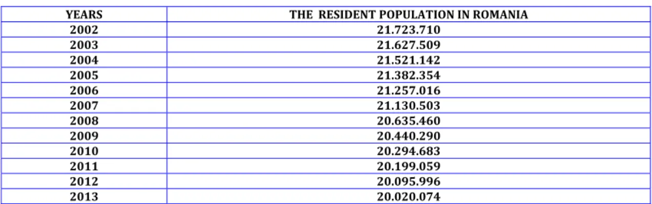
)n the period - , we observe the next evolution concerning the resident population in Romania, according to the table no. :

Table 1 The evolution of the resident population in Romania, between 2002-2013 YEARS THE RESIDENT POPULATION IN ROMANIA

2002 21.723.710 2003 21.627.509 2004 21.521.142 2005 21.382.354 2006 21.257.016 2007 21.130.503 2008 20.635.460 2009 20.440.290 2010 20.294.683 2011 20.199.059 2012 20.095.996 2013 20.020.074

Source: „Romanian international migration 2014”, page no. 33, I.N.S.S.E., Bucharest.

First, we want to identify the trend model for the resident population in Romania, in the period - , using the table no. .

- if we formulate the null hypothesis

H

0: which mentions the assumption of the existence for the model of

tendency of the factor X = the resident population in Romania, as being the function

x

_t

a

b

t

_i

i

=

+

⋅

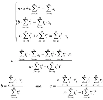
, then the

parameters a and b of the adjusted linear function, can to be calculated by means of the next system [ ]:

⎪

⎪

⎩

⎪⎪

⎨

⎧

⋅

=

⋅

=

⋅

∑

∑

∑

− = − =

− =

m

m i

i i m

m i

i m

m i

i

x

t

t

b

x

a

n

2

Therefore,

n

x

a

m

m i

i

∑

− =

=

and

∑

∑

− = − =

⋅

=

m

m i

i m

m i

i i

t

x

t

b

2

Table 2 The estimate of the value for the variation coefficient in the case of the adjusted linear function, in the hypothesis concerning the linear evolution of the

resident population in Romania, between the years 2002-2013

LINEAR TREND YEARS

THE RESIDENT POPULATION

IN ROMANIA

(xi)

t

i

2

i

t

t

_i

x

_i

x

_t

a

bt

_i

i

=

+

x

i

−

x

ti

2002 21.723.710 - - , ,

2003 21.627.509 - - , ,

2004 21.521.142 - - , ,

2005 21.382.354 - - , ,

2006 21.257.016 - - , ,

2007 21.130.503 - - , ,

2008 20.635.460 , ,

2009 20.440.290 , ,

2010 20.294.683 , ,

2011 20.199.059 , ,

2012 20.095.996 , ,

2013 20.020.074 , ,

TOTAL 250.327.796 - . . , . ,

)f we calculate the statistical data for to adjust the linear function, we obtain for the parameters a and b the values:

6666

,

20860649

12

250327796

=

=

a

156918

,

79670

182

28559221

−

=

−

=

b

(ence, the coefficient of variation for the adjusted linear function is:

%

32

,

0

100

796

.

327

.

250

5934

,

211

.

800

100

100

:

_⋅

₌

_⋅

₌

−

=

⋅

⎥

⎥

⎥

⎥

⎦

⎤

⎢

⎢

⎢

⎢

⎣

⎡

−

=

∑

∑

∑

∑

− = − = −

= −

=

m

m i

i m

m i

I t i m

m i

i m

m i

I t i I

x

x

x

n

x

n

x

x

v

i i

- in the situation of the alternative hypothesis

H

1 : which specifies the assumption of the existence for the

model of tendency of the factor X = the resident population in Romania, as being the quadratic function

2

i i t

a

b

t

ct

x

i

=

+

⋅

+

, the parameters a, b şi c of the adjusted quadratic function, can to be calculated by means

⎪

⎪

⎪

⎩

⎪

⎪

⎪

⎨

⎧

⋅

=

+

⋅

⋅

=

⋅

=

+

⋅

∑

∑

∑

∑

∑

∑

∑

− = − = − = − = − = − = − = m m i i i m m i i m m i i m m i i i m m i i m m i i m m i i

x

t

t

c

t

a

x

t

t

b

x

t

c

a

n

2 4 2 2 2 Consequently,

∑

∑

∑

∑

∑

∑

− = − = − = − = − = − =

−

⋅

⋅

⋅

−

⋅

=

m m i i m m i i m m i i i m m i i m m i i m m i i

t

t

n

x

t

t

x

t

a

2 2 4 2 2 4

)

(

∑

∑

− = − =

⋅

=

m m i i m m i i i

t

x

t

b

2 and

∑

∑

∑

∑

∑

− = − = − = − = − =

−

⋅

⋅

−

⋅

⋅

=

m m i i m m i i m m i i m m i i m m i i i

t

t

n

x

t

x

t

n

c

2 2 4 2 2

)

(

Table 3. The estimates of the value for the variation coefficient in the case of the adjusted quadratic function, in the hypothesis concerning the parabolic evolution of the resident population in Romania,

between the years 2002-2013

PARABOLIC TREND

YEARS

THE RESIDENT POPULATION

IN ROMANIA

(xi)

t

i

2

i

t

t

_i4

t

_i2

x

_i

x

_t

a

bt

_i

ct

_i2

i

=

+

+

x

i

−

x

ti

2002 21.723.710 - , ,

2003 21.627.509 - , ,

2004 21.521.142 - , ,

2005 21.382.354 - , ,

2006 21.257.016 - , ,

2007 21.130.503 - , ,

2008 20.635.460 , ,

2009 20.440.290 , ,

2010 20.294.683 , ,

2011 20.199.059 , ,

2012 20.095.996 , ,

2013 20.020.074 , ,

TOTAL 250.327.796 ,

)f we calculate the statistical data for to adjust the quadratic function, we obtain for the parameters a,b and c the next values:

3305085

,

20857282

33124

4550

12

3797035585

182

250327796

4550

.

9

=

−

⋅

⋅

−

⋅

=

a

79670

,

156918

182

28559221

−

=

−

=

b

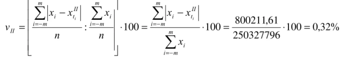
So, the coefficient of variation for the adjusted quadratic function has the value:

%

32

,

0

100

250327796

61

,

800211

100

100

:

⋅

=

⋅

=

−

=

⋅

⎥

⎥

⎥

⎥

⎦

⎤

⎢

⎢

⎢

⎢

⎣

⎡

−

=

∑

∑

∑

∑

− = − = −

= −

=

m

m i

i m

m i

II t i m

m i

i m

m i

II t i II

x

x

x

n

x

n

x

x

v

i i

- in the case of the alternative hypothesis

H

₂ : which describes the supposition the assumption of the existence for the model of tendency of the factor X = the resident population in Romania, as being the exponential function i

i

t t

ab

x

₌

_{, then the parameters} a and b of the adjusted exponential function, can to be calculated by means of the next system [ ]:

⎪

⎪

⎩

⎪⎪

⎨

⎧

⋅

=

⋅

=

⋅

∑

∑

∑

− = −

= − =

m

m i

i i m

m i

i m

m i

i

x

t

t

b

x

a

n

lg

lg

lg

lg

2

Thus,

n

x

a

m

m i

i

∑

− =

=

lg

lg

and

∑

∑

− = − =

⋅

=

_m

m i

i m

m i

i i

t

x

t

b

2

lg

lg

Table 4 The estimate of the value for the variation coefficient in the case of the adjusted exponential function, in the hypothesis concerning the exponential evolution of

the resident population in Romania, between 2002-2013

EXPONENTIAL TREND

YEARS

THE RESIDENT POPULATION

IN ROMANIA

(xi) i

t

lg

x

_i

t

_i

lg

x

_i

=

ti

x

lg

b t

a _ilg

lg ₊

=

x

ti

=

ab

ti i ti

x

x

₋

2002 21.723.710 - , - , , , ,

2003 21.627.509 - , - , , , ,

2004 21.521.142 - , - , , , ,

2005 21.382.354 - , - , , , ,

2006 21.257.016 - , - , , , ,

2007 21.130.503 - , - , , , ,

2008 20.635.460 , , , , ,

2009 20.440.290 , , , , ,

2010 20.294.683 , , , , ,

2011 20.199.059 , , , , ,

2012 20.095.996 , , , , ,

2013 20.020.074 , , , , ,

TOTAL 250.327.796 , - , ,

Consequently, if we calculate the statistical data for to adjust the exponential function, we obtain for the parameters a and b the values:

0

,

003268007

182

59477734

,

0

lg

b

₌

−

₌

₋

319138608

,

7

12

82966329

,

87

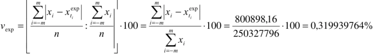
Accordingly, the coefficient of variation for the adjusted exponential function has the next value:

%

319939764

,

0

100

250327796

16

,

800898

100

100

:

exp exp

exp

⋅

=

⋅

=

−

=

⋅

⎥

⎥

⎥

⎥

⎦

⎤

⎢

⎢

⎢

⎢

⎣

⎡

−

=

∑

∑

∑

∑

− = − = −

= −

=

m

m i

i m

m i

t i m

m i

i m

m i

t i

x

x

x

n

x

n

x

x

v

i i

We apply the coefficients of variation method as criterion of selection for the best model of trend. We notice that:

%

319939764

,

0

%

319665503

,

0

%

319665497

,

0

_<

₌

_<

_exp

₌

=

v

v

v

_{I II}

So, the path reflected by X factor, which represents the resident population in Romania, between

2002-2013, is a linear trend of the shape

x

_t

a

bt

_i

i

=

+

, with other words it confirms the hypothesis

H

0.

20000000 21000000 22000000

2002 2003 2004 2005 2006 2007 2008 2009 2010 2011 2012 2013

THE LINEAR TREND OF THE RESIDENT POPULATION IN ROMANIA, IN THE PERIOD 2002-2013

Figure 1. The trend model of the values for the resident population in Romania, in the period 2002-2013

We observe that, the cloud of points which reflects the values of the resident population in Romania, between - , it carrying around a linear model of trend, according to the type no. .

3. The modeling of the trend concerning the all romanian population, in the period 2000-2013.

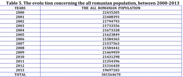
Table 5. The evolu tion concerning the all romanian population, between 2000-2013

YEARS THE ALL ROMANIAN POPULATION

2000 22435205 2001 22408393 2002 21794793 2003 21733556 2004 21673328 2005 21623849 2006 21584365 2007 21537563 2008 21504442 2009 21469959 2010 21431298 2011 21354396 2012 21316420 2013 19697103 TOTAL 301564670

The sourse: „Romania in dates , page. no. , ).N.S.S.E., Bucharest

- if we formulate the null hypothesis * 0

H

: which mentions the assumption of the existence for the model of tendency of the factor Y = the all romanian population, as being the function

y

_t

a

b

t

_i

i

=

+

⋅

, then the

parameters a and b of the adjusted linear function, can to be calculated by means of the next system [ ]:

⎪

⎪

⎩

⎪⎪

⎨

⎧

⋅

=

⋅

=

⋅

∑

∑

∑

− = −

= − =

m

m i

i i m

m i

i m

m i

i

y

t

t

b

y

a

n

2

Therefore,

n

y

a

m

m i

i

∑

− =

=

and

∑

∑

− = − =

⋅

=

_m

m i

i m

m i

i i

t

y

t

b

2

Table 6. The estimate of the value for the variation coefficient in the case of the adjusted linear function, in the hypothesis concerning the linear evolution for the all romanian population,

between the years 2000-2013

LINEAR TREND YEARS

THE ALL ROMANIAN POPULATION

(yi)

t

_i

t

_i2

t

_i

y

_i

y

_t

a

bt

_i

i

=

+

y

i

−

y

t_i

2000 - - , ,

2001 - - , ,

2002 - - , ,

2003 - - , ,

2004 - - , ,

2005 - - , ,

2006 - - , ,

2007 , ,

2008 , ,

2009 , ,

2010 , ,

2011 , ,

2012 , ,

2013 , ,

So, the parameters a and b have the next the values:

21540333

,

57

14

301564670

=

=

a

107233

,

1857

280

30025292

−

=

−

=

b

Consequently, the coefficient of variation for the adjusted linear function is:

%

3217

,

1

100

301564670

84

,

3985745

100

100

:

_⋅

₌

_⋅

₌

−

=

⋅

⎥

⎥

⎥

⎥

⎦

⎤

⎢

⎢

⎢

⎢

⎣

⎡

−

=

∑

∑

∑

∑

− = − = − = − = m m i i m m i I t i m m i i m m i I t i I

y

y

y

n

y

n

y

y

v

i i

- in the situation of the alternative hypothesis * 1

H

: which specifies the assumption of the existence for the model of tendency of the factor Y = the all romanian population, as being the quadratic function

2

i i t

a

b

t

ct

y

i

=

+

⋅

+

, the parameters a, b şi c of the adjusted quadratic function, can to be calculated by

means of the system [ ]:

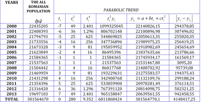
Table 7. The estimates of the value for the variation coefficient in the case of the adjusted quadratic function, in the hypothesis concerning the parabolic evolution of the all romanian population,

between the years 2000-2013

PARABOLIC TREND

YEARS THE ALL

ROMANIAN POPULATION

(yi)

t

i

2

i

t

t

_i4

t

_i2

y

_i

y

_t

a

bt

_i

ct

_i2

i

=

+

+

y

i

−

y

ti

2000 - . , ,

2001 - . , ,

2002 - , ,

2003 - , ,

2004 - , ,

2005 - , ,

2006 - , ,

2007 , ,

2008 , ,

2009 , ,

2010 , ,

2011 , ,

2012 . , ,

2013 . , ,

TOTAL . , ,

)f we calculate the statistical data for to adjust the second function, we obtain for the parameters a,b and c the next values:

220

,

21643878

400

.

78

352

.

9

14

6011868424

280

301564670

9352

=

−

⋅

⋅

−

⋅

=

a

186

,

107233

280

30025292

−

=

−

=

b

5177

,

232

400

.

78

352

.

9

14

301564670

280

6011868424

14

−

=

−

⋅

⋅

−

⋅

=

c

So, the coefficient of variation for the adjustedquadratic function has the value:

%

38

,

1

100

301564670

25

,

4148417

100

100

:

_⋅

₌

_⋅

₌

−

=

⋅

⎥

⎥

⎥

⎥

⎦

⎤

⎢

⎢

⎢

⎢

⎣

⎡

−

=

∑

∑

∑

∑

− = − = −

= −

=

m

m i

i m

m i

II t i m

m i

i m

m i

II t i II

y

y

y

n

y

n

y

y

v

i i

- in the case of the alternative hypothesis

H

₂* : which describes the supposition the assumption of the existence for the model of tendency of the factor Y = the all romanian population,as being the exponential function i

i

t t

ab

y

₌

, then the parameters a and b of the adjusted exponential function, can to be calculated by means of the next system [ ]:

⎪

⎪

⎩

⎪⎪

⎨

⎧

⋅

=

⋅

=

⋅

∑

∑

∑

− = −

= − =

m

m i

i i m

m i

i m

m i

i

y

t

t

b

y

a

n

lg

lg

lg

lg

Thus,

n

y

a

m

m i

i

∑

− =

=

lg

lg

and

∑

∑

− = − =

⋅

=

_m

m i

i m

m i

i i

t

y

t

b

2

lg

lg

Table 8. The estimate of the value for the variation coefficient in the case of the adjusted exponential function, in the hypothesis concerning the exponential evolution of the all romanian population,

between the years 2000-2013

A. EXPONENTIAL TREND

YEARS

THE ALL ROMANIAN POPULATION

(yi) i

t

lg

y

i

i i

y

t

lg

=

ti

y

lg

b t

a _ilg

lg ₊

=

y

ti

=

ab

ti

y

i

−

y

ti

2000 - , - , , , ,

2001 - , - , , , ,

2002 - , - , , , ,

2003 - , - , , , ,

2004 - , - , , , ,

2005 - , - , , , ,

2006 - , - , , , ,

2007 , , , , ,

2008 , , , , ,

2009 , , , , ,

2010 , , , , ,

2011 , , , , ,

2012 , , , , ,

2013 , , , , ,

TOTAL , - , ,

Consequently, if we calculate the statistical data for to adjust the exponential function, we obtain for the parameters a and b the values:

0

,

00218773

280

612564535

,

0

lg

b

=

−

=

−

The coefficient of variation for the adjusted exponential function has the next value

:

%

3275

,

1

100

301564670

43

,

4003383

100

100

:

exp exp

exp

⋅

=

⋅

=

−

=

⋅

⎥

⎥

⎥

⎥

⎦

⎤

⎢

⎢

⎢

⎢

⎣

⎡

−

=

∑

∑

∑

∑

− = − = −

= −

=

m

m i

i m

m i

t i m

m i

i m

m i

t i

x

y

y

n

y

n

y

y

v

i i

We observe that:

v

_I

₌

1

,

3217

%

_<

v

_exp

₌

1

,

3275

%

_<

v

_II

₌

1

,

38

%

So, the path followed by Y factor, which represents the all romanian population, between 2000-2013,

is a linear trend of the shape

y

_t

a

bt

_i

i

=

+

, with other words it confirms the hypothesis

* 0

H

.

333073609

,

7

14

6630305

,

102

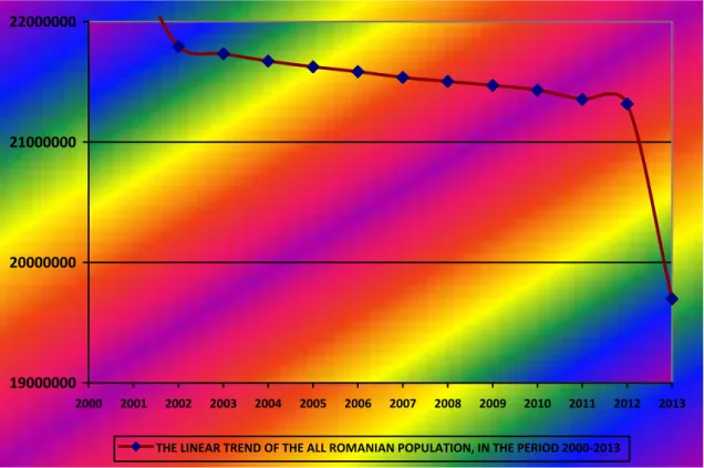
19000000 20000000 21000000 22000000

2000 2001 2002 2003 2004 2005 2006 2007 2008 2009 2010 2011 2012 2013

THE LINEAR TREND OF THE ALL ROMANIAN POPULATION, IN THE PERIOD 2000-2013

Figure 2. The model of trend concerning the values for the all romanian population, in the period 2000-2013

So, the cloud of points which reflects the values concerning the all romanian population, between - , it carrying around a linear trend model, according to the type no. .

4. The forecasting method through the „Least Squares Method”

We know that the evolution of the resident population in Romania reflects a linear trend of the shape

i t

a

bt

x

i

=

+

. So, in , the resident population in Romania will be:

POPULATION

₂₀₁₄RESIDENT

₌

20860649

,

6666

₊

(

₋

156918

,

79670

)

_⋅

7

₌

19

.

762

.

218

,

09

inhabitants

POPULATION

₂₀₁₅RESIDENT

₌

20860649

,

6666

₊

(

₋

156918

,

79670

)

_⋅

8

₌

19

.

605

.

299

,

29

inhabitans

POPULATION

₂₀₁₆RESIDENT

₌

20860649

,

6666

₊

(

₋

156918

,

79670

)

_⋅

9

₌

19

.

448

.

380

,

49

inhabitans

POPULATION

₂₀₁₇RESIDENT

₌

20860649

,

6666

₊

(

₋

156918

,

79670

)

_⋅

10

₌

19

.

291

.

461

,

69

inhabitans

POPULATION

₂₀₁₈RESIDENT

₌

20860649

,

6666

₊

(

₋

156918

,

79670

)

_⋅

11

₌

19

.

134

.

542

,

90

inhabitans

POPULATION

₂₀₁₉RESIDENT

₌

20860649

,

6666

₊

(

₋

156918

,

79670

)

_⋅

12

₌

18

.

977

.

624

,

10

inhabitans

POPULATION

₂₀₂₀RESIDENT

₌

20860649

,

6666

₊

(

₋

156918

,

79670

)

_⋅

13

₌

18

.

820

.

705

,

30

_inhabitans

Also, the trend of the all romanian population is a linear trend of the shape

x

ti

=

a

+

bt

i. Thus, in , the

total of the romanian population will be:

POPULATION

₂₀₁₅ROMANIA

₌

21540333

,

57

₊

(

₋

107233

,

1857

)

_⋅

9

₌

20

.

575

.

234

,

90

people

POPULATION

₂₀₁₆ROMANIA

₌

21540333

,

57

₊

(

₋

107233

,

1857

)

_⋅

10

₌

20

.

468

.

001

,

71

people

POPULATION

₂₀₁₇ROMANIA

₌

21540333

,

57

₊

(

₋

107233

,

1857

)

_⋅

11

₌

20

.

360

.

768

,

53

people

POPULATION

₂₀₁₈ROMANIA

=

21540333

,

57

+

(

−

107233

,

1857

)

⋅

12

=

20

.

253

.

535

,

34

people

2019

=

21540333

,

57

+

(

−

107233

,

1857

)

⋅

13

=

20

.

146

.

302

,

16

ROMANIA

POPULATION

_people

2020

=

21540333

,

57

+

(

−

107233

,

1857

)

⋅

14

=

20

.

039

.

068

,

97

ROMANIA

POPULATION

_people

5. Conclusions

We can to synthesize that the evolution in future concerning the resident population in Romania, respectively the all romanian population is in a continuously decreasing. As we can see, The romanian population decreased in , under million inhabitants as against , million in , changing percent during the last years. According to The National )nstitute of Statistics from Bucharest, if the rate is maintained, Romania's population will decline by with about million inhabitants.

References

1. Gauss C. F. - „Theoria Combinationis Observationum Erroribus Minimis Obnoxiae”, Apud Henricum Dieterich Publising House, Gottingae, 1823.

2. Kariya T., Kurata H. - „Generalized Least Squares”, John Wiley&Sons Publishing House, Hoboken, 2004.

3. Rao Radhakrishna C., Toutenburg H., Fieger A., Heuman C., Nittner T., Scheid S. - „Linear Models: Least Squares and Alternatives”, Springer Series in Statistics, Springer-Verlag New York – Berlin Heidelberg Publishing House, New-York, 1999.

4. Robertson T. - „The Malthusian Moment – global population growth”, Rutgers University Press Publishing House, 2012.