www.clim-past.net/7/235/2011/ doi:10.5194/cp-7-235-2011
© Author(s) 2011. CC Attribution 3.0 License.
of the Past
A new mechanism for the two-step
δ
18
O signal at the
Eocene-Oligocene boundary
M. Tigchelaar1,*, A. S. von der Heydt1, and H. A. Dijkstra1
1Institute for Marine and Atmospheric Research Utrecht, Utrecht University, Utrecht, The Netherlands
*current at: School of Ocean and Earth Science and Technology, University of Hawaii at M¯anoa, Honolulu, Hawaii, USA Received: 2 July 2010 – Published in Clim. Past Discuss.: 21 July 2010
Revised: 25 January 2011 – Accepted: 7 February 2011 – Published: 9 March 2011
Abstract.The most marked step in the global climate transi-tion from “Greenhouse” to “Icehouse” Earth occurred at the Eocene-Oligocene (E-O) boundary, 33.7 Ma. Evidence for climatic changes comes from many sources, including the marine benthicδ18O record, showing an increase by 1.2– 1.5‰ at this time. This positive excursion is characterised by two steps, separated by a plateau. The increase inδ18O values has been attributed to rapid glaciation of the Antarc-tic continent, previously ice-free. Simultaneous changes in theδ13C record are suggestive of a greenhouse gas control on climate. Previous modelling studies show that a decline inpCO2 beyond a certain threshold value may have initi-ated the growth of a Southern Hemispheric ice sheet. These studies were not able to conclusively explain the remark-able two-step profile inδ18O. Furthermore, they considered changes in the ocean circulation only regionally, or indi-rectly through the oceanic heat transport. The potential role of global changes in ocean circulation in the E-O transition has not been addressed yet. Here a new interpretation of the
δ18O signal is presented, based on model simulations using a simple coupled 8-box-ocean, 4-box-atmosphere model with an added land ice component. The model was forced with a slowly decreasing atmospheric carbon dioxide concentra-tion. It is argued that the first step in theδ18O record reflects a shift in meridional overturning circulation from a Southern Ocean to a bipolar source of deep-water formation, which is associated with a cooling of the deep sea. The second step in theδ18O profile occurs due to a rapid glaciation of the Antarctic continent. This new mechanism is a robust out-come of our model and is qualitatively in close agreement with proxy data.
Correspondence to:M. Tigchelaar
1 Introduction
While the long-term variations in our present-day climate are paced by the waxing and waning of the Northern Hemi-spheric ice sheet, Earth’s surface was (almost) entirely ice-free at the beginning of the Cenozoic Era, 65.5 Ma. In the course of this Era, Earth’s climate experienced a transition from a “Greenhouse” world to the current “Icehouse” world, the most marked step of which occurred close to the Eocene-Oligocene (E-O) boundary, 33.7 Ma. The Eocene climate was relatively warm, with polar surface and deep water tem-peratures up to 10◦
C warmer than today. The Antarctic con-tinent – though in its present position – was ice-free and lushly vegetated. At the E-O boundary, global temperatures dropped and a semi-permanent ice-sheet formed on Antarc-tica. An overwhelming amount of evidence from fossils and proxies indicates that climate change at the E-O boundary was global and involved all parts of the climate system (Lear et al., 2000; DeConto and Pollard, 2003a; Dockery and Lo-zouet, 2003; Hay et al., 2005; Zachos and Kump, 2005; Cox-all and Pearson, 2007; Liu et al., 2009).
The most pronounced evidence for relatively rapid cli-matic changes comes from the marineδ18O record. Numer-ous cores taken from the ocean floor display an abrupt in-crease inδ18O of 1.2–1.5‰ across the E-O boundary. The shift lasts approximately 500 kyr and is characterised by a re-markable two-step profile in which two 40-kyr steps are sep-arated by a plateau of 200 kyr. The E-O transition terminates with a sustained maximum persisting for 400 kyr, followed by several stepped decreases (Coxall et al., 2005). Eventu-ally δ18O values stabilise ∼31 Ma to a value∼1‰ higher than before the transition (Zachos et al., 1996; Zachos and Kump, 2005; Coxall and Pearson, 2007).
Although Northern Hemispheric ice rafted debris dating back to the middle Eocene has also been found, data are insuf-ficient to determine the extent of a Northern Hemisphere glaciation at this time (Eldrett et al., 2007). It is highly likely that a rapid glaciation of the Antarctic continent was accom-panied by a (local) decrease in temperature and there are many indications that theδ18O signal comprises both an ice volume and a temperature change (Oerlemans, 2004; Cox-all and Pearson, 2007; de Boer et al., 2010). Analysis of the Mg/Ca-ratio in benthic foraminifera indicates a cooling of up to 2.5◦C in the tropics (Lear et al., 2000, 2004, 2008). UK′ 37 and TEX86 analyses have lead to the conclusion that high-latitude sea surface temperatures (SSTs) decreased by 4.8– 5.4◦C from the late Eocene to the early and mid-Oligocene. Model simulations show that such a decrease in SSTs corre-sponds to a decrease in deep-water temperatures of 3–5◦C. Combining this result with theδ18O record produces maxi-mum ice volume estimates of 40–120% of modern Antarctic ice volume (Liu et al., 2009).
Changes in the global carbon cycle are reflected in the
δ13C record, which displays a rapid and stepwise increase of 1‰ similar in shape and duration to the shift observed in
δ18O values. The increase inδ13C is thought to be indicative of enhanced marine export production (Zachos and Kump, 2005; Coxall and Pearson, 2007). The sharp rise of carbon isotope ratios has also been associated with a two-step deep-ening of the carbon compensation depth (CCD) by more than 1 km (Rea and Lyle, 2005; Zachos and Kump, 2005). The CCD is linked to ocean acidity, which is in turn linked to atmospheric CO2concentration (Coxall et al., 2005; Merico et al., 2008). Proxy records show a general decline inpCO2 throughout the Cenozoic from 2–5 times pre-industrial at-mospheric levels (PAL) in the mid-Eocene, to near-modern values in the lower Miocene, although sufficient detail to ac-curately determine the CO2decline across the E-O boundary is lacking (Pagani et al., 2005; Coxall and Pearson, 2007; Pearson et al., 2009).
During the Eocene, the Southern Ocean and even mid-latitudes are thought to have played a greater role in deep-water formation. Sedimentary and seismic evidence in com-bination with analysis of neodymium (Nd) isotopes shows that there was a transition from a southern sinking source to a bipolar source of deep-water formation at the beginning of the Oligocene (Thomas et al., 2003; Thomas, 2004; Via and Thomas, 2006). The initiation of deep water forma-tion in the North Atlantic was facilitated by the subsidence of the Greenland-Scotland Ridge which may have occurred around the E-O boundary (Davies et al., 2001). Other im-plied climatic changes include an increased latitudinal tem-perature gradient, more powerful atmospheric circulation, higher aridity and changes in seasonality (Coxall et al., 2005; Eldrett et al., 2009).
Currently two main hypotheses explaining the complex E-O climate transition abide; one involves the opening of ocean gateways around the E-O boundary, the other uses
de-clining CO2 values below a certain threshold value as the main driver. The opening of Drake Passage between Antarc-tica and South America and of Tasmanian Passage between Antarctica and Australia has facilitated the organisation of the Antarctic Circumpolar Current (ACC), reducing south-ward oceanic heat transport and cooling Southern Ocean SSTs. Since the opening of these passages occurred around the E-O boundary, it might have played a dominant role in the glaciation of Antarctica. Precise timing of the opening of these gateways has, however, proven to be problematic (Liv-ermore et al., 2005; Scher and Martin, 2006; Coxall and Pear-son, 2007). Evidence to support a vigourous ACC before the mid-Miocene is scarce (Coxall and Pearson, 2007). Further-more, DeConto and Pollard (2003a) argue that the influence of colder Southern Ocean SSTs on Antarctic meteorology is poorly resolved, and Huber and Nof (2006) demonstrate that ocean heat transport would have had to decrease enormously for any significant changes in Antarctic continental tempera-tures to occur.
Huber and Nof (2006) argue additionally that the ma-jor changes in productivity during the E-O transition are strong evidence in favour of a greenhouse gas control on climate. It has been proposed that, once some CO2 thresh-old (∼750 ppm, Pearson et al., 2009) was reached, feed-backs related to snow/ice-albedo and ice-sheet height/mass-balance could have initiated rapid ice-sheet growth (DeConto and Pollard, 2003a,b; Coxall and Pearson, 2007). DeConto and Pollard (2003a) ran a global climate model coupled to a dynamic ice-sheet model, forcing it with a CO2 decline from 4 to 2 times PAL in 10 Myr. They found that rela-tively small ice caps form due to high levels of winter pre-cipitation, which start to grow rapidly beyond some thresh-old CO2 concentration and eventually coalesce to form one continental scale ice-sheet. In their simulations with a non-dynamical, 50-m slab ocean, the opening of Drake Passage only affects the timing of ice-sheet growth. Other modelling and data studies support the idea that the opening of Drake Passage and the subsequent development of the ACC may have helped ice growth on Antarctica but was not the ulti-mate cause (Sijp and England, 2004; Sijp et al., 2009; Cramer et al., 2009; Haywood et al., 2010). It is thought that the initi-ation and rapid growth of the ice-sheet is aided by the specific orbital settings at the E-O boundary: low eccentricity and low-amplitude changes in obliquity favour dampened sea-sonality and cold summers (DeConto and Pollard, 2003a,b; Coxall et al., 2005; Coxall and Pearson, 2007).
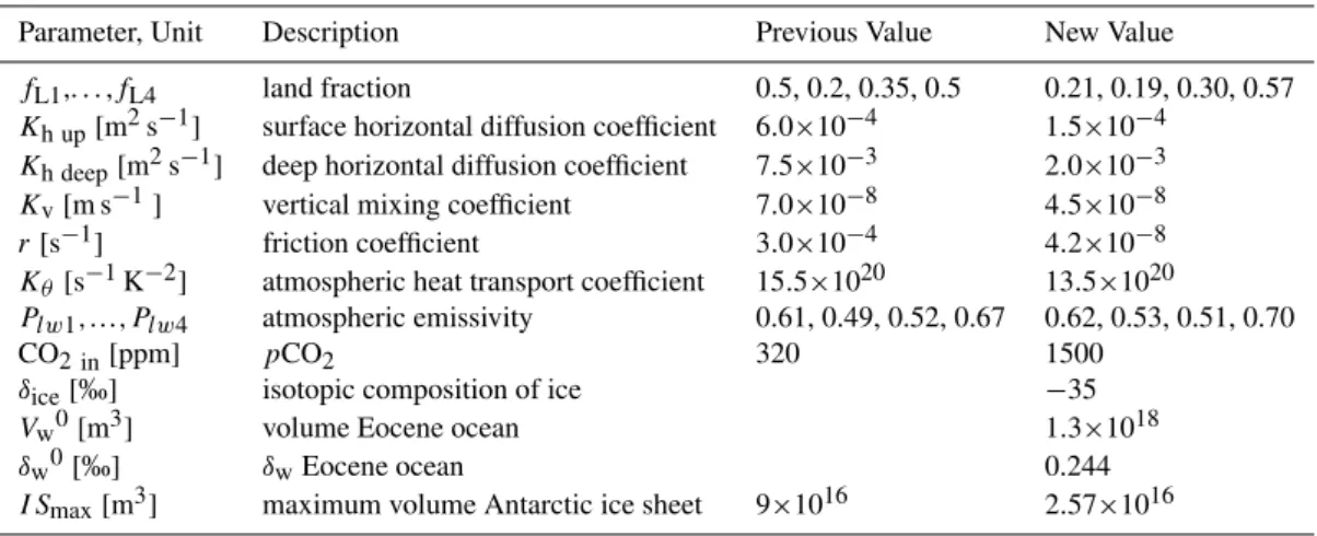
Table 1.Parameters that were changed from or added to Gildor et al. (2002).
Parameter, Unit Description Previous Value New Value
fL1,. . . ,fL4 land fraction 0.5, 0.2, 0.35, 0.5 0.21, 0.19, 0.30, 0.57 Kh up[m2s−1] surface horizontal diffusion coefficient 6.0×10⁻⁴ 1.5×10⁻⁴
Kh deep[m2s−1] deep horizontal diffusion coefficient 7.5×10⁻³ 2.0×10⁻³ Kv[m s−1] vertical mixing coefficient 7.0×10⁻⁸ 4.5×10⁻⁸ r[s−1] friction coefficient 3.0×10⁻⁴ 4.2×10⁻⁸ Kθ[s−1K−2] atmospheric heat transport coefficient 15.5×10²⁰ 13.5×10²⁰
Plw1,...,Plw4 atmospheric emissivity 0.61, 0.49, 0.52, 0.67 0.62, 0.53, 0.51, 0.70
CO2 in[ppm] pCO2 320 1500
δice[‰] isotopic composition of ice −35
Vw0[m3] volume Eocene ocean 1.3×10¹⁸
δw0[‰] δwEocene ocean 0.244
I Smax[m3] maximum volume Antarctic ice sheet 9×10¹⁶ 2.57×10¹⁶
Here a new mechanism explaining the two δ18O steps across the E-O transition record will be presented in which several parts of the climate system are involved and switches in the MOC play a dominant role. The transition from “Greenhouse” to “Icehouse” is simulated using an adapted version of the model developed by Gildor and Tziperman (2000, 2001) and Gildor et al. (2002). This model is a cou-pled 8-box-ocean, 4-box-atmosphere model with added land ice and sea ice components, the details of which will be briefly described in Sect. 2. In a model of such simplicity, the role and importance of the different mechanisms at work are (more) easily distinguishable.
In Sect. 3 it is argued that the first increase inδ18O val-ues represents (mostly) cooling of the deep sea. This cooling is brought about by a switch in the MOC from a southern sinking state to a bipolar sinking state. The secondδ18O step reflects the growth of the Antarctic ice sheet and further cool-ing as a result of this. The crucial control parameter induc-ing the two-step transition is the atmospheric carbon dioxide concentration. As will be shown in Sect. 4, our new mech-anism is a robust outcome of the model and qualitatively in close agreement with proxy data.
2 The model
The model that is used is an adapted version of the coupled ocean-atmosphere-ice model that was developed by Gildor and Tziperman (2000, 2001) and Gildor et al. (2002) to ex-plain the 100-kyr period observed in glacial-interglacial os-cillations for the past 400 kyr. To this model we added a mod-ule to compute changes inδ18O. By changing the parame-ters of the model, it can be adapted to paleoclimatic bound-ary conditions (see below). In this section the most impor-tant characteristics of the model are discussed; a full descrip-tion of the equadescrip-tions can be found in Gildor and Tziperman
(2001) and Gildor et al. (2002). An overview of the param-eters that were altered with respect to Gildor et al. (2002) is presented in Table 1.
The ocean is represented by four surface boxes and four deep boxes whose latitudinal extends are South Pole to 45◦
S, 45◦
S to equator, equator to 45◦
N and 45◦
N to North Pole. The meridional overturning circulation is buoyancy driven; advection and diffusion of temperature and salinity are bal-anced by surface fluxes from the atmosphere and land ice components. The atmospheric model consists of four verti-cally averaged boxes representing the same latitude bands as the ocean boxes. The surface below the atmospheric boxes is a combination of ocean, land, land ice and sea ice, each with its specified albedo. The averaged potential tempera-ture in the box is calculated on the basis of the energy bal-ance in the box, consisting of: incoming solar radiation, using box albedo and with the possibility to include Mi-lankovitch variations; outgoing long-wave radiation; heat-flux into the ocean; and meridional atmospheric heat trans-port. The meridional atmospheric moisture transport is pro-portional to the meridional temperature gradient and the hu-midity of the box to which the flux is directed. Precipitation is calculated as the convergence of the moisture fluxes.
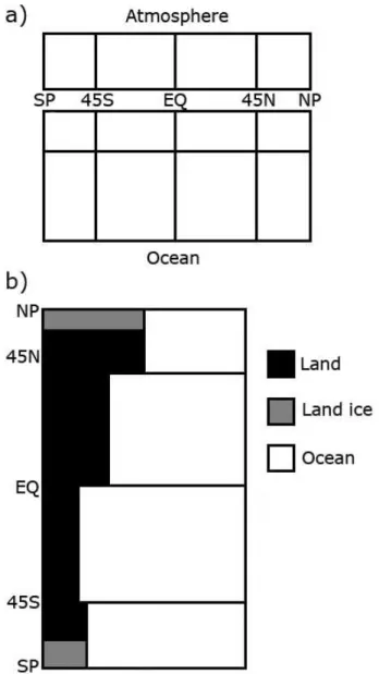
Fig. 1. Box model (a) meridional cross section (b) top view. Adapted from Gildor and Tziperman (2001).
A known problem of many models, including this one, is a too high sensitivity to the sea ice-albedo feedback. This means that when the ocean covers a large proportion of the box (≥80%), the feedback mechanism will cause the ocean to be completely sea ice covered. Especially in the most southern box, where land fractions are low, this is prob-lematic. Therefore – since there are no indications that sea ice changes played a dominant role in the Eocene-Oligocene transition (Huber and Sloan, 2001) – the sea ice component is left out of the study entirely to allow land fractions to take on realistic values. Hence, there will be no sea ice present in all boxes.
An additional module was added to the model that com-putes variations inδ18O. The oxygen isotopic composition of sea-waterδwis calculated using the volumetric changes in
land ice and ocean and conservation of totalδ18O (Bintanja et al., 2005; de Boer et al., 2010):
Vw0×δw0=Vice×δice+Vw×δw (1) whereVw0is the volume of the Eocene ocean, andVwis the volume of the ocean after ice formation:Vw=Vw0−Vice.δice is the isotopic composition of land ice and δw0 andδw are the isotopic compositions of the Eocene ocean and the ocean after ice formation, respectively. The values that were used for these variables can be found in Table 1.
The sea-water isotopic compositionδw together with the simulated temperature T (in ◦
C) of the four lower ocean boxes is then used to calculate the calcite isotopic com-position δc according to the calcite-temperature relation of Shackleton (1974):
T=16.9−4.38(δc−δw)+0.1(δc−δw)2 (2) The initial Eocene value δw0 is chosen such that the mod-elled Eocene deep sea temperature matches the measured late Eocene calcite isotopic composition. The prognostic equa-tions in the model are solved using a leapfrog time scheme with a uniform time step of 6 h. All variables are aver-aged over 200 years (Gildor and Tziperman, 2001). For the present study biogeochemical feedback processes are ignored.
3 Results
3.1 The Eocene reference state
First the model was adapted to paleoclimatic boundary con-ditions representing those of the Eocene climate system. The largest differences between the climatic boundary conditions for which the model was developed (Gildor and Tziperman, 2000, 2001; Gildor et al., 2002) and those of the Eocene cli-mate, are the position of the continents and the background atmospheric greenhouse gas concentrations. Therefore in the model the land fraction per box and pCO2 were adjusted. Representative values for the land fractions were obtained from Markwick et al. (2000) and can be found in Table 1. A CO2 concentration was sought for which the land ice would disappear (almost) entirely, while not (excessively) exceeding the upper-limit of 5 times PAL as set by Pagani et al. (2005).
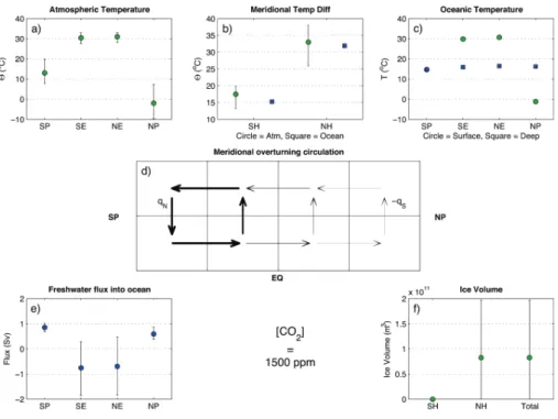
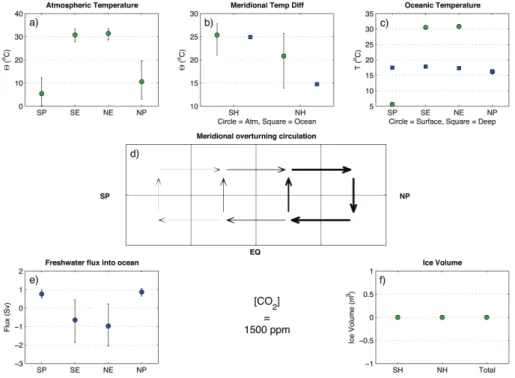
Fig. 2. Overview of the modelled state of the Eocene climate at a CO2concentration of 1500 ppm with the MOC in the SPP pattern;
(a)atmospheric temperature for the southern polar (SP), southern equatorial (SE), northern equatorial (NE) and northern polar (NP) boxes;
(b)meridional temperature difference for the Southern Hemisphere (SH) and Northern Hemisphere (NH) for the atmosphere (circles) and ocean (squares);(c)oceanic temperature of surface waters (circles) and deep sea (squares);(d)southern sinking MOC where the direction of the arrows indicates the direction of volume transport and their thickness indicates the magnitude;(e)freshwater flux into the ocean;(f)ice volume on the Southern Hemisphere (SH), Northern Hemisphere (NH) and in total; markers represent yearly averaged values, error bars indicate the seasonality.
The yearly averaged atmospheric temperature (Fig. 2a) is slightly over 30◦
C in the equatorial boxes, around 13◦ C in the southern box and just below freezing in the northern box. Subsequently, the atmospheric meridional temperature gradi-ent (Fig. 2b) in the Northern Hemisphere is quite high, while taking on a more moderate value in the South. A similar pat-tern can be observed in the yearly averaged surface ocean temperatures (Fig. 2c). The oceanic meridional tempera-ture gradients are therefore comparable to the atmospheric ones. In the polar boxes the seasonality is much higher (10– 15◦
C) than in the equatorial boxes (5◦
C). The yearly aver-aged freshwater flux into the ocean (Fig. 2e) is positive in the polar boxes and negative in the equatorial boxes; i.e., there is evaporation at the equator and precipitation at the poles. The seasonality of the freshwater flux is much higher at the equator than at the poles.
To check the validity of this reference state, the ocean tem-perature results are compared with Eocene data from Bijl et al. (2009) and Liu et al. (2009), and GCM model results from Huber and Sloan (2001). In the southern and equato-rial boxes, modelled SSTs are in reasonable agreement with measurements. However, proxy data as well as the GCM results indicate that both poles were relatively warm (up to 20◦
C) during the Eocene. Simulated northern box temper-atures are therefore too cold. Liu et al. (2009) measured
deep-sea temperatures of∼10◦
C. Deep-sea temperatures in our modelled reference state are therefore too warm. Too high deep sea temperatures are a known problem of ocean box models. Values for the freshwater flux into the ocean were compared against modern-day observations (Oberhu-ber, 1988) and these are of the same order of magnitude, so the model determines realistic values of the buoyancy flux. 3.2 Critical threshold for continental ice formation
0 200 400 600 800 1000 0
500 1000 1500 2000
[CO
2
] (ppm)
a)
1 2
0 200 400 600 800 1000 0
2 4 6 8 10x 10
16
Ice Volume (m
3)
b)
0 200 400 600 800 1000 −20
−10 0 10 20 30 40
Time (103 years)
Potential temperature (
oC)
c)
0 200 400 600 800 1000 −1
−0.5 0 0.5 1
Time (103 years)
Freshwater flux (Sv)
d)
Fig. 3.Effect of(a)changing CO2concentrations on(b)ice volume in the southern polar box and(c)atmospheric temperature and(d) fresh-water flux in the southern polar box (dark blue), southern equatorial box (green), northern equatorial box (red) and northern polar box (light blue). On the left (1 in a) is the simulation with linearly decreasingpCO2, and on the right (2 in a)pCO2is raised back to its initial value and stabilises there.
The response of the climate system to decreasing carbon dioxide concentrations differs per box. At first, when no ice sheet is formed yet, the temperature decrease as plotted in Fig. 3c shows a similar pattern across the globe: slowly at first, but more rapidly aspCO2 continues to fall. The in-ception of the Southern Hemispheric ice sheet lowers atmo-spheric temperatures in the most southern polar box and the southern equatorial box additionally through the ice-albedo feedback, while northern temperatures are barely affected. During the transition, the northern meridional temperature difference decreases, while the southern difference increases, especially after the ice sheet has started to grow. The amount of equatorial evaporation and polar precipitation decreases, see Fig. 3d.
It was also tested whether the climate system returns to its initial state whenpCO2is raised back to 1500 ppm. The Antarctic ice sheet starts to melt at 605 ppm, a value well above the CO2 concentration of ice inception. The differ-ence in criticalpCO2 levels is due to the ice-albedo feed-back which lowers the atmospheric temperature as long as the ice sheet is present. It takes∼300 kyr for the ice sheet to melt entirely, and this is a linear rather than an exponential process.
Changes in temperature and freshwater flux in the north-ern boxes under increasing CO2are a mirrored version of the
response to decreasing CO2described above: temperatures increase at a decreasing rate. The response in the southern boxes follows the melting of the Antarctic ice sheet and is therefore linear. Once the CO2concentration has returned to 1500 ppm and the climate system is restored to equilibrium, the global temperature and freshwater distributions are ex-actly the same as they were before the transition. The south-ern sinking state of the MOC remains unaffected throughout the transition. When the rate ofpCO2decrease is doubled or halved the results remain qualitatively the same.
3.3 Existence of multiple climate equilibria
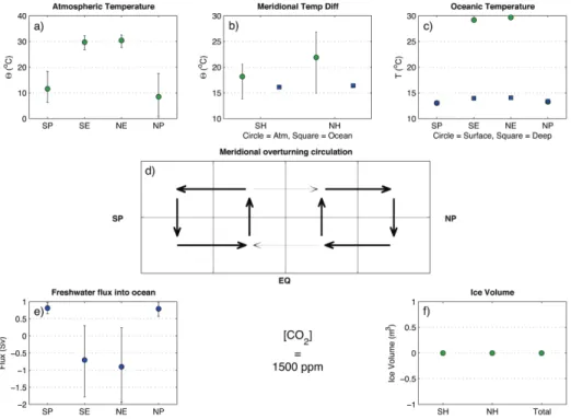
Fig. 4. Overview of the modelled state of the Eocene climate at a CO2concentration of 1500 ppm with the MOC in the TH pattern;
(a)atmospheric temperature for the southern polar (SP), southern equatorial (SE), northern equatorial (NE) and northern polar (NP) boxes;
(b)meridional temperature difference for the Southern Hemisphere (SH) and Northern Hemisphere (NH) for the atmosphere (circles) and ocean (squares);(c)oceanic temperature of surface waters (circles) and deep sea (squares);(d)bipolar sinking MOC where the direction of the arrows indicates the direction of volume transport and their thickness indicates the magnitude;(e)freshwater flux into the ocean;(f)ice volume on the Southern Hemisphere (SH), Northern Hemisphere (NH) and in total; markers represent yearly averaged values, error bars indicate the seasonality.
poles (TH), and upwelling at both poles (SA). Whether the solutions are stable depends on the boundary conditions (i.e. parameter settings) of the model. Since our ocean model is similar to the models just described, it is expected that multiple steady state solutions might exist in our Eocene cli-mate. Indeed, for the Eocene boundary conditions a TH state (Fig. 4d) and NPP state (Fig. 5d) are also found to be sta-ble solutions of the model, in addition to the SPP state found earlier (Fig. 2d).
The state of the MOC affects the global temperature dis-tribution: compare Fig. 2 to Figs. 4 and 5. In the NPP and TH states there is more oceanic heat transport towards the North than in the SPP state; consequently, northern atmo-spheric and sea surface temperatures are higher, leading to the disappearance of the Arctic ice sheet. Northerly SSTs are in these states more in accordance with the Bijl et al. (2009) and Liu et al. (2009) data and Huber and Sloan (2001) GCM results. Similarly, southern atmospheric and sea surface tem-peratures in the NPP state are lower as a result of a decrease in heat transport. This lowering is insufficient to initiate the growth of an Antarctic ice sheet. Deep sea temperatures are coldest in the TH state (13.6◦C, Fig. 4c) and warmest in the NPP state (17.2◦C, Fig. 5c).
The simulations with changingpCO2(Sect. 3.2) showed that even if global atmospheric temperatures change
drasti-cally, the SPP state of the Eocene reference state persists. To investigate the stability of all the MOC states under decreas-ing CO2 concentrations, the model was run for each state withpCO2decreasing with 100 ppm increments. For every CO2concentration the model was run until the system was in equilibrium. The pattern and strength of the MOC can be deduced from the value ofqN−qS, where qN (qS) is the volume transport from the surface layer to the deep ocean in the northern (southern) box (Fig. 2d). AqN−qSthat is posi-tive indicates a NPP state, a negaposi-tiveqN−qSindicates a SPP state and ifqN−qSis approximately zero the ocean is in a TH state. In Fig. 6aqN−qSis plotted against atmospheric CO2 concentration. This bifurcation diagram shows that the SPP and the TH state of the overturning circulation coexist for all values ofpCO2. This is not the case for the NPP state, which ceases to exist for CO2concentrations lower than 1400 ppm. At these lower concentrations the NPP state can no longer be sustained due to a strengthening of the freshwater input into the northern polar box.
Fig. 5. Overview of the modelled state of the Eocene climate at a CO2concentration of 1500 ppm with the MOC in the NPP pattern;
(a)atmospheric temperature for the southern polar (SP), southern equatorial (SE), northern equatorial (NE) and northern polar (NP) boxes;
(b)meridional temperature difference for the Southern Hemisphere (SH) and Northern Hemisphere (NH) for the atmosphere (circles) and ocean (squares);(c)oceanic temperature of surface waters (circles) and deep sea (squares);(d)northern sinking MOC where the direction of the arrows indicates the direction of volume transport and their thickness indicates the magnitude;(e)freshwater flux into the ocean;(f)ice volume on the Southern Hemisphere (SH), Northern Hemisphere (NH) and in total; markers represent yearly averaged values, error bars indicate the seasonality.
3.4 Transitions between equilibria
The fact that the SPP and TH states coexist for the entire range of CO2concentrations between 100 and 1500 ppm in-dicates that it is possible for the climate system to switch between these states. Such a shift would be in accordance with data that show that the MOC at the E-O boundary changed from a Southern Ocean to a bipolar source of deep-water formation (Thomas et al., 2003; Thomas, 2004; Via and Thomas, 2006; Coxall and Pearson, 2007). Therefore it is tested whether it is possible to initiate such a transition in the model.
A transition from the SPP state to the TH state is induced at a CO2concentration of 800 ppm by adding a density per-turbation to the surface layer in the northern polar box. This perturbation lasts for a short time (200 year, i.e. one aver-aging time-step) and is of small magnitude (1 kg m−3) com-pared to the background density. The immediate result is that water in this box starts to sink. Subsequently, heavier water dominating the artificial perturbation is advected and causes the MOC to change to the TH state. When the CO2 con-centration is lowered further, the system remains on the TH branch (Fig. 6a). The ability of the system to switch between MOC states exists for all CO2 concentrations. Transitions between MOC states as a result of a finite amplitude density
perturbation therefore can always occur due to noise in the climate system.
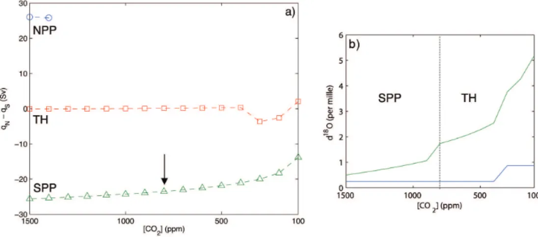
The correspondingδ18O profile (Fig. 6b) consists of two rapid increases, separated by a plateau. The first of these shifts represents the transition in the MOC from the SPP to the TH state. Deep sea temperatures in the TH state are colder than in the SPP state (compare Fig. 4c to 2c), be-cause polar surface waters are colder in the North than in the South. At colder temperatures, the calciteδ18O value (δc) is higher. During the shift, the modelled increase inδ18O is 0.67‰, which corresponds to a deep sea temperature de-crease of 2.8◦
Fig. 6. (a)Simulated bifurcation diagram showing pattern and strength of the MOC for different initial states: NPP (circles), TH (squares) and SPP (triangles). The arrow denotes the CO2concentration at which the small density perturbation in the northern surface box was applied.
(b)Simulatedδ18O profile when a density perturbation is applied to the SPP MOC in the northern surface box at a CO2concentration of 800 ppm. Theδ18O profile is separated into the contribution due to changes in ice volume (δw, blue) and the total signal with the added effect of deep sea temperature changes (δc, green). The first shift inδcrepresents the transition in the MOC from the SPP to the TH state, the second shift represents Antarctic ice growth.
Inception of ice growth on the Southern Hemisphere in our model occurs at CO2 concentrations below 400 ppm. This is very low compared to the measurements of Pear-son et al. (2009) and model studies by DeConto and Pol-lard (2003a,b), who estimated Antarctic ice growth to start at 750 ppm. A possible explanation for the relatively low CO2 concentration of ice inception in the model is that the ice sheet only grows if the temperature in the polarboxrather thanatthe pole is below 0◦
C. Since the box temperature is an average, it will already be far below freezing at the pole when this threshold is reached. Therefore, thepCO2of ice inception might be raised by increasing the inception temper-ature of ice in the model.
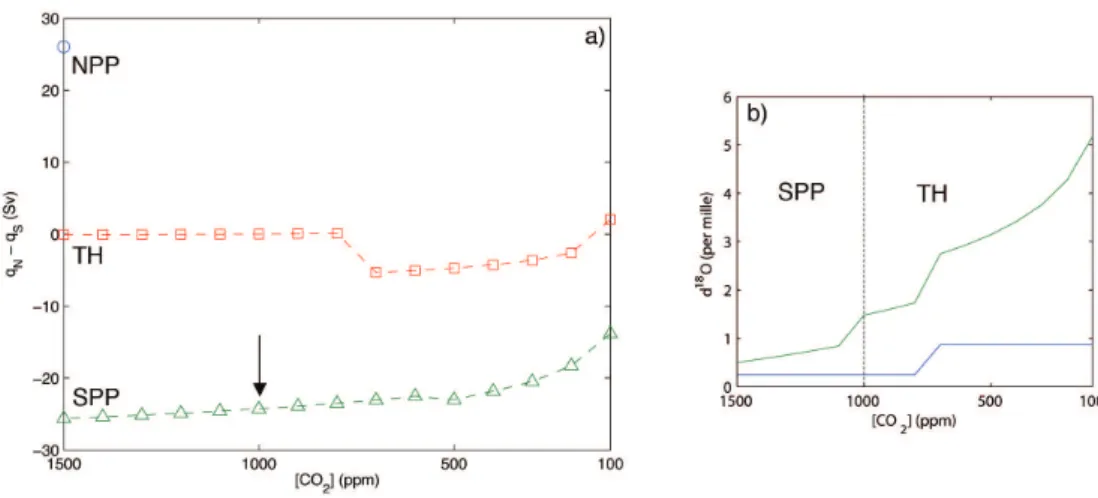
The first test was done by raising the inception temperature of ice to 3◦C. Ice growth now occurs for CO2concentrations lower than 800 ppm. It is again possible to initiate a transi-tion from the SPP to the TH state by perturbing the density. This can be done at anypCO2≥800 ppm; here we chose to place the perturbation at 1000 ppm. The resulting bifurcation diagram is shown in Fig. 7a. Again, theδ18O shift (Fig. 7b) exhibits a two-step profile. Both steps are slightly smaller than the steps in Fig. 6b. These results show that it is indeed possible to improve thepCO2of ice inception in the model.
When the inception temperature is raised even higher, to 5◦
C, the Eocene reference state with the MOC in the SPP pattern ceases to exist. Therefore there must exist an incep-tion temperature between 3 and 5◦C for which the SPP state ceases to exist at a CO2concentration lower than 1500 ppm and higher than thepCO2 of Antarctic ice inception. For this inception temperature, the transition from the SPP to the TH state – and hence the two-stepδ18O profile – will spon-taneously occur in the model.
4 Summary and discussion
Global cooling and the initiation of the Antarctic ice sheet at the E-O boundary 33.7 Ma are thought to be the result of decreasing atmospheric carbon dioxide levels below a cer-tain threshold value. Thus far, the remarkable two-step pro-file of theδ18O record at this boundary has remained unex-plained. For the late Eocene, proxy data indicate a south-ern sinking state of the meridional overturning circulation (MOC). Deep water formation in the northern high latitudes of the Atlantic Ocean as it is formed in the modern climate may have been initiated in the early Oligocene, possibly fa-cilitated by tectonic changes such as the subsidence of the Greenland-Scotland Ridge (Davies et al., 2001). The role of MOC changes during the E-O climate transition has not yet been investigated. Therefore an adapted version of the simple coupled 8-box-ocean, 4-box-atmosphere model with added land ice component by Gildor and Tziperman (2000, 2001) and Gildor et al. (2002) was used to simulate the re-sponse of the full climate system to a decrease inpCO2.
Fig. 7.Same as Fig. 6 but with the inception temperature of ice increased to 3◦C:(a)Simulated bifurcation diagram showing pattern and strength of the MOC for different initial states: NPP (circles), TH (squares) and SPP (triangles). The arrow denotes the CO2concentration at which the small density perturbation in the northern surface box was applied.(b)Simulatedδ18O profile when a density perturbation is applied to the SPP MOC in the northern surface box at a CO2concentration of 1000 ppm. Theδ18O profile is separated into the contribution due to changes in ice volume (δw, blue) and the total signal with the added effect of deep sea temperature changes (δc, green). The first shift inδcrepresents the transition in the MOC from the SPP to the TH state, the second shift represents Antarctic ice growth.
The NPP state ceases to exist for CO2 concentrations lower than 1400 ppm. Both the SPP and the TH pattern ex-ist for all levels ofpCO2between 100 and 1500 ppm. This suggests that it is possible for the system to switch between these MOC states. The switch in overturning state leads to a cooling of the deep sea and hence a positive excursion of
δ18O values. The second step in theδ18O record can be in-terpreted as representing the rapid glaciation of the Antarctic ice sheet.
In our model, a transition from the SPP to the TH state was induced by means of a small density perturbation. In reality, a switch between different MOC states may be induced by various mechanisms: given the small value of the density perturbation necessary to induce the MOC transition, it may be induced by (random) fluctuations in the strength of the hydrological cycle. Alternatively, tectonic changes, which have not been considered here, may initiate or at least help to establish another MOC pattern. In particular, two tectonic events have been timed around the E-O boundary, which may have facilitated a transition to NH deep water formation:
i. The subsidence of the Greenland-Scotland Ridge may have facilitated North Atlantic deep water formation (Davies et al., 2001; Abelson et al., 2008).
ii. The possible development of an unrestricted (but most likely still very shallow) Antarctic circumpolar zonal flow by the opening of the Tasman Gateway and Drake Passage around the E-O boundary may decrease the strength of Southern Hemisphere deep water formation via the geostrophic balance and in turn facilitate North-ern Hemisphere deep water formation. Many previ-ous modeling studies have shown that Southern Ocean
deep water formation is reduced when there exists an unrestricted zonal circum-Antarctic flow (Mikolajewicz et al., 1993; Toggweiler and Samuels, 1995); this ef-fect is often referred to as the “Drake Passage efef-fect”. In Dijkstra et al. (2003) the different Atlantic MOC states were investigated in a three dimensional ocean model with an open and closed southern channel. In that study the “Drake Passage effect” leads to a prefer-ence of a state with northern sinking when opening the southern channel (see their Fig. 5). When considering the temperature change due to the establishment of an Antarctic circumpolar flow, the Southern Ocean SSTs cool, while the northern hemispheric SSTs warm (Tog-gweiler and Bjornsson, 2000; Nong et al., 2000; Sijp and England, 2004). In view of the study by Dijkstra et al. (2003) at least part of the Southern Ocean cool-ing is due to a transition from one MOC state with more southern deep water formation to one with more north-ern deep water formation. The opening of Drake Pas-sage and the establishment of a first (weak) Antarctic Circumpolar Current could therefore have induced the SPP to TH transition (as accomplished in our box model by a (small) density perturbation) because of the prefer-ence for northern sinking.
While the opening of gateways may have helped to induce a transition in the MOC pattern, the timing of these gateway changes remains controversial. It is therefore interesting to repeat here that in our model a very small density perturba-tion is enough to induce the transiperturba-tion.
an inception temperature of 3◦C (averaged over the entire southern polar box) ice growth is initiated below 800 ppm. This is in close agreement with data and modelling studies. For an ice inception temperature of 5◦
C, the Eocene refer-ence state with the MOC in a SPP pattern ceases to exist. This suggests that an inception temperature between 3 and 5◦
C exists for which the transition from the SPP to the TH state under decreasingpCO2occurs spontaneously.
Despite the fact that a model of very low complexity was used to simulate the Eocene-Oligocene transition, our new interpretation of theδ18O record appears to be coherent and complies qualitatively well with proxy data. Quantitative model-data comparisons, however, are difficult in this con-text and should be done with caution. Due to the model’s simplistic representation of radiative transfer, model CO2 should be thought of as only representing rough changes in radiative forcing. The exact values of the threshold CO2 con-centrations for ice formation as found in DeConto and Pol-lard (2003a,b) and DeConto et al. (2008) model studies can therefore not directly be compared as they depend on model parameters. The same holds for CO2reconstructions (Pagani et al., 2005; Pearson et al., 2009), which themselves contain large uncertainties.
The exact timing of the modelled shifts and intermittent plateau is still undetermined and is largely dependent on the exact pattern ofpCO2change. The total magnitude of the two modelled steps is slightly larger than the estimates from
δ18O proxy records. This can be attributed to the second step – representing Antarctic ice growth – being overesti-mated. In our model simulations, the Southern Hemispheric ice sheet was allowed to grow to its full size, 2.57×10¹⁶m3, the present-day size of the Antarctic ice sheet. This is on the high end of the maximum E-O ice volume estimates (40– 120% of modern Antarctic ice volume, Liu et al., 2009). It takes the ice sheet∼100 kyr to grow to this size, while data indicate that the second step only lasted for 40 kyr. Therefore there must have been a mechanism that stopped the growth of the Antarctic ice sheet after 40 kyr. This mechanism might be related to the CO2record, which is known to have dis-played variable rates of changes around the E-O boundary. According to measurements by Pearson et al. (2009), there might even have been a temporary increase in CO2 concen-trations during the second step, which could have stabilised the growth of the ice sheet.
Northern polar temperatures in our modelled Eocene ref-erence state were found to be too cold, and deep sea temper-atures were found to be too warm. These discrepancies be-tween modelled temperatures and data are a shortcoming of the model. The too cold Northern polar temperatures in our model can be attributed to the lack of Northern Hemispheric deep water formation and consequently reduced oceanic heat transport to northern high latitudes. The box model does not include the wind-driven ocean circulation, which is par-tially responsible for oceanic meridional heat transport, so meridional heat transport differences due to the locations of
deep water formation are overestimated. In a more realis-tic model, the temperature difference between northern and southern high latitudes in a southern sinking pattern of the MOC would therefore be less severe. The data of Liu et al. (2009) do suggest slightly colder Northern Hemisphere SSTs than in the Southern Hemispherebeforethe E-O transition. Furthermore, an increased seasonality in northern high lat-itudes before the Oi-1 event as suggested by Eldrett et al. (2009) would also support relatively cool NH winter SSTs.
Although changes in MOC and ice volume under decreas-ing CO2concentrations prove to be a plausible explanation for the observed δ18O signal, possible mechanisms behind thepCO2 decline remain unaddressed. In our model study atmosphericpCO2was a prescribed forcing and not an out-put variable. Proposed causes of the CO2 decline in the literature are reduced sea-floor spreading, increased silicate weathering, increased marine production and release of or-ganic carbon from geological reservoirs (Zachos and Kump, 2005; Coxall and Pearson, 2007; Pearson et al., 2009). Posi-tive feedback mechanisms exist between these processes and the changes in MOC and ice volume found in our simula-tions. The role and strength of these mechanisms could be tested with the biogeochemical module developed by Gildor et al. (2002) or the more comprehensive models of Zachos and Kump (2005) and Merico et al. (2008), but are outside the scope of this paper.
In this model study, only a limited number of feedback processes has been incorporated. These processes have proven to be sufficient to newly interpret theδ18O record at the E-O boundary. Nonetheless, the results of this research will be even more robust when they can be reproduced us-ing more complex models. The role of several potentially important processes should be investigated in the future. To fully understand the influence of the opening of oceanic gate-ways, a full three-dimensional ocean model should be used in which (i) Southern Ocean dynamics are included and an ACC can be formed, (ii) separate Atlantic and Pacific ocean basins are included with varying connections between them, and (iii) the dynamics of the overflow at the Greenland-Scotland ridge is accounted for. It will also be interesting to see how the changes described here affect atmospheric circu-lation patterns, and vice versa. Although the land ice module used in this study is very simple, its results are in qualitative agreement with those in DeConto and Pollard (2003a,b). Of course, the precise details of Antarctic ice sheet formation can be better understood from their simulations. Changes in orbital configuration were not taken into account in our simulations, even though they are thought to have played a significant role.
step represents rapid Antarctic ice growth, caused by lower-ing of the atmospheric carbon dioxide levels below a certain threshold level. The two-step signature will always occur when the MOC transition – which can occur spontaneously due to random density perturbations or can be induced by tec-tonic changes – occurs at higherpCO2levels than the criti-calpCO2level for Southern Hemispheric ice formation. The mechanisms that are proposed here are qualitatively in close agreement with proxy data, and so is the order of magnitude of the two modelledδ18O steps.
Acknowledgements. We thank Hezi Gildor for kindly providing us
with the model used in this study and helping us with the set-up. We also thank Helen Coxall and Dorian Abbot for their constructive and insightful reviews, the Editor for valuable comments, and Bas de Boer and Roderik van de Wal for fruitful discussions.
Edited by: G. Lohmann
References
Abelson, M., Agnon, A., and Almogi-Labin, A.: Indications for control of the Iceland plume on the Eocene-Oligocene “greenhouse-icehouse” climate transition, Earth Planet. Sci. Lett., 265, 33–48, 2008.
Bijl, P. K., Schouten, S., Sluijs, A., Reichart, G.-J., Zachos, J. C., and Brinkhuis, H.: Early Palaeogene temperature evolution of the Southwest Pacific Ocean, Nature, 461, 776–779, 2009. Bintanja, R., van de Wal, R. S. W., and Oerlemans, J.: Modelled
atmospheric temperatures and global sea levels over the past mil-lion years, Nature, 437, 125–128, 2005.
Coxall, H. K. and Pearson, P. N.: The Eocene-Oligocene Transi-tion, in: Deep-Time Perspectives on Climate Change: Marry-ing the Signal from Computer Models and Biological Proxies, edited by: Williams, M., Haywood, A. M., Gregory, F. J., and Schmidt, D. N., 351–387, The Micropalaeontological Society Special Publication, 2007.
Coxall, H. K., Wilson, P. A., P¨alike, H., Lear, C. H., and Back-man, J.: Rapid stepwise onset of Artarctic glaciation and deeper calcite compensation in the Pacific Ocean, Nature, 433, 53–57, 2005.
Cramer, B. S., Toggweiler, J. R., Wright, J. D., Katz, M. E., and Miller, K. G.: Ocean overturning since the Late Cretaceous: In-ferences from a new benthic foraminiferal isotope compilation, Paleoceanography, 24, PA4216, doi:10.1029/2008PA001683, 2009.
Davies, R., Cartwright, J., Pike, J., and Line, C.: Early Oligocene Initiation of North Atlantic Deep Water Formation, Nature, 410, 917–920, 2001.
de Boer, B., van de Wal, R., Bintanja, R., Lourens, L., and Tuenter, E.: Cenozoic global ice-volume and temperature simulations with 1-D ice-sheet models forced by benthicδ18O records, An-nals of Glaciology, 51, 23–33, 2010.
DeConto, R. M. and Pollard, D.: Rapid Cenozoic glaciation of Antarctica induced by declining atmospheric CO2, Nature, 421, 245–249, 2003a.
DeConto, R. M. and Pollard, D.: A coupled climate-ice sheet mod-eling approach to the Early Cenozoic history of the Antarctic ice sheet, Palaeogeogr. Palaeocl., 198, 39–52, 2003b.
DeConto, R. M., Pollard, D., Wilson, P. A., P¨alike, H., Lear, C. H. and Pagani, M.: Thresholds for Cenozoic bipolar glaciation, Na-ture, 455, 652–656, 2008.
Dijkstra, H. A., Weijer, W., and Neelin, J. D.: Imperfections of the three-dimensional thermohaline ocean circulation: Hystere-sis and unique state regimes, J. Phys. Oceanogr., 33, 2796–2814, 2003.
Dockery, D. and Lozouet, P.: Biotic patterns in Eocene-Oligocene Molluscs of the Atlantic Coastal Plain, USA, in: From Green-house to IceGreen-house, edited by: Prothero, D. R., Ivany, L., and Nesbitt, E. A., 303–340, Columbia University Press, 2003. Eldrett, J. S., Harding, I. C., Wilson, P. A., Butler, E., and Roberts,
A. P.: Continental ice in Greenland during the Eocene and Oligocene, Nature, 446, 176–179, 2007.
Eldrett, J. S., Greenwood, D. R., Harding, I. C., and Huber, M.: Increased seasonality through the Eocene to Oligocene transition in northern high latitudes, Nature, 459, 969–974, doi:10.1038/nature08069, 2009.
Ghil, M., Mulhaupt, A., and Pestiaux, P.: Deep water formation and Quaternary glaciations, Clim. Dyn., 2, 1–10, 1987.
Gildor, H. and Tziperman, E.: Sea ice as the glacial cycles’ climate switch: role of seasonal and orbital forcing, Paleoceanography, 15, 605–615, 2000.
Gildor, H. and Tziperman, E.: A sea ice climate switch mechanism for the 100-kyr glacial cycles, J. Geophys. Res., 106, 9117–9133, 2001.
Gildor, H., Tziperman, E., and Toggweiler, J.: Sea ice switch mechanism and glacial-interglacial CO2variations, Global Bio-geochem. Cy., 16, GB0203, doi:10.1029/2001GB001446, 2002. Hay, W. W., Fl¨ogel, S., and S¨oding, E.: Is the initiation of glaciation on Antarctica related to a change in the structure of the ocean?, Global Planet. Change, 45, 23–33, 2005.
Haywood, A., Valdes, P., Lunt, D., and Pekar, S.: The Eocene-Oligocene boundary and the Antarctic Circumpolar Current, in: Geophysical Research Abstracts, vol. 12, pp. EGU2010–5031, 2010.
Huber, M. and Nof, D.: The ocean circulation in the southern hemisphere and its climate impacts in the Eocene, Palaeogeogr. Palaeocl., 231, 9–28, 2006.
Huber, M. and Sloan, L. C.: Heat transport, deep waters, and ther-mal gradients: coupled simulation of an Eocene greenhouse cli-mate, Geophys. Res. Lett., 28, 3481–3484, 2001.
IPCC: Climate Change 2007: the Physical Science Basis. Contribu-tion of Working Group I to the Fourth Assessment Report of the Intergovernmental Panel on Climate Change, Cambridge Uni-versity Press, Cambridge, United Kingdom and New York, NY, USA, 2007.
Lear, C. H., Elderfield, H., and Wilson, P. A.: Cenozoic deep-sea temperatures and global ice volumes from Mg/Ca in benthic foraminiferal calcite, Science, 287, 269–272, 2000.
Lear, C. H., Rosenthal, Y., Coxall, H. K., and Wilson, P. A.: Late Eocene to early Miocene ice-sheet dynamics and the global carbon cycle, Paleoceanography, 19, PA4015, doi:10.1029/2004PA001039, 2004.
transition, Geology, 36, 251–254, 2008.
Liu, Z., Pagani, M., Zinniker, D., DeConto, R., Huber, M., Brinkhuis, H., Shah, S. R., Leckie, R. M., and Pearson, A.: Global cooling during the Eocene-Oligocene climate transition, Science, 323, 1187–1190, 2009.
Livermore, R., Nankivell, A., Eagles, G., and Morris, P.: Paleogene opening of Drake passage, Earth Planet. Sc. Lett., 236, 459–470, 2005.
Markwick, P. J., Rowley, D. B., Ziegler, A. M., Hulver, M. L., Valdes, P. J., and Sellwood, B. W.: Late Cretaceous and Ceno-zoic global palaeogeographies: Mapping the transition from a “hot-house” to an “ice-house” world, GFF, 122, p. 103, 2000. Merico, A., Tyrrell, T., and Wilson, P. A.: Eocene/Oligocene ocean
de-acidification linked to Antarctic glaciation by sea-level fall, Nature, 452, 979–982, 2008.
Mikolajewicz, U., Maier-Reimer, E., Crowley, T., and Kim, K.: Ef-fects of Drake and Panamanian Gateways on the circulation of an ocean model, Paleoceanograpy, 8, 409–426, 1993.
Nong, G. T., Najjar, R. G., Seidov, D., and Peterson, W. H.: Simula-tion of Ocean Temperature Change due to the Opening of Drake Passage, Geophys. Res. Lett., 27, 2689–2692, 2000.
Oberhuber, J. M.: An atlas based on “COADS” data set, Tech. Rep. 15, Max-Planck-Institut f¨ur Meteorologie, 1988.
Oerlemans, J.: Correcting theδ18O deep-sea temperature record for Antarctic ice volume, Palaeogeogr. Palaeocl., 208, 195–205, 2004.
Pagani, M., Zachos, J. C., Freeman, K. H., Tipple, B., and Bo-haty, S.: Marked decline in atmospheric carbon dioxide concen-trations during the paleogene, Science, 309, 600–603, 2005. Pearson, P. N., Foster, G. L., and Wade, B. S.: Atmospheric
car-bon dioxide through the Eocene-Oligocene climate transition, Nature, 461, 1110–1113, 2009.
Rea, D. K. and Lyle, M. W.: Paleogene calcite compensation depth in the eastern subtropical Pacific: answers and questions, Paleo-ceanography, 20, PA1012, doi:10.1029/2004PA001064, 2005. Scher, H. D. and Martin, E. E.: Timing and climatic consequences
of the opening of Drake passage, Science, 312, 428–430, 2006. Shackleton, N. J.: Attainment of isotopic equilibrium between
ocean water and the benthonic foraminifera genus Uvigerina: isotopic changes in the ocean during the last glacial, C. N. R. S. Colloq., 219, 203–209, 1974.
Sijp, W. P., England, M. H., and Toggweiler, J. R.: Effect of Ocean Gateway Changes under Greenhouse Warmth, J. Climate, 22, 6639–6652, doi:10.1175/2009JCLI3003.1, 2009.
Sijp, W. and England, M.: Effect of the Drake Passage throughflow on global climate, J. Phys. Oceanogr., 34, 1254–1266, 2004. Stommel, H.: Thermohaline convection with two stable regimes of
flow, Tellus, 13, 224–230, 1961.
Thomas, D. J.: Evidence for deep-water production in the North Pacific Ocean during the early Cenozoic warm interval, Nature, 430, 65–68, 2004.
Thomas, D. J., Bralower, T. J., and Jones, C. E.: Neodymium iso-topic reconstruction of late Paleocene-early Eocene thermohaline circulation, Earth Planet. Sc. Lett., 209, 309–322, 2003. Thual, O. and McWilliams, J. C.: The catastrophe structure of
thermohaline convection in a two-dimensional fluid model and a comparison with low-order box models, Geophys. Astro. Fluid, 64, 67–95, 1992.
Toggweiler, J. R. and Bjornsson, H.: Drake Passage and Paleocli-mate, J. Quat. Sci., 15, 319–328, 2000.
Toggweiler, J. R. and Samuels, B.: Effect of Drake Passage on the global thermohaline circulation, Deep-Sea Res., 42, 477–500, 1995.
Via, R. K. and Thomas, D. J.: Evolution of Atlantic thermohaline circulation: Early Oligocene onset of deep-water production in the North Atlantic, Geology, 34, 441–444, 2006.
Welander, P.: Thermohaline effects in the ocean circulation and related simple models, in: Large-Scale Transport Processes in Oceans and Atmosphere, edited by: Willebrand, J. and Ander-son, D. L. T., 163–200, D. Reidel, 1986.
Williams, Jr., R. S. and Ferrigno, J. G.: Satellite Image Atlas of Glaciers of the World, USGS Fact Sheet 2005–3056, 2005. Zachos, J. C. and Kump, L. R.: Carbon cycle feedbacks and the
initiation of Antarctic glaciation in the earliest Oligocene, Global Planet. Change, 47, 51–66, 2005.