BGD
9, 11843–11883, 2012
Controls on the spatial distribution of
oceanicδ13C DIC
P. B. Holden et al.
Title Page
Abstract Introduction
Conclusions References
Tables Figures
◭ ◮
◭ ◮
Back Close
Full Screen / Esc
Printer-friendly Version
Interactive Discussion
Discussion
P
a
per
|
Dis
cussion
P
a
per
|
Discussion
P
a
per
|
Discussio
n
P
a
per
|
Biogeosciences Discuss., 9, 11843–11883, 2012 www.biogeosciences-discuss.net/9/11843/2012/ doi:10.5194/bgd-9-11843-2012
© Author(s) 2012. CC Attribution 3.0 License.
Biogeosciences Discussions
This discussion paper is/has been under review for the journal Biogeosciences (BG). Please refer to the corresponding final paper in BG if available.
Controls on the spatial distribution of
oceanic
δ
13
C
DIC
P. B. Holden1, N. R. Edwards1, S. A. M ¨uller2, K. I. C. Oliver2, R. M. Death3, and A. Ridgwell3
1
Environment, Earth and Ecosystems, Open University, Milton Keynes, UK 2
Ocean and Earth Science, National Oceanography Centre Southampton, University of Southampton, Southampton, UK
3
School of Geographical Sciences, University of Bristol, Bristol, UK
Received: 30 July 2012 – Accepted: 16 August 2012 – Published: 31 August 2012
Correspondence to: P. B. Holden (p.b.holden@open.ac.uk)
BGD
9, 11843–11883, 2012
Controls on the spatial distribution of
oceanicδ13C DIC
P. B. Holden et al.
Title Page
Abstract Introduction
Conclusions References
Tables Figures
◭ ◮
◭ ◮
Back Close
Full Screen / Esc
Printer-friendly Version
Interactive Discussion
Discussion
P
a
per
|
Dis
cussion
P
a
per
|
Discussion
P
a
per
|
Discussio
n
P
a
per
|
Abstract
We describe the design and evaluation of a large ensemble of coupled climate-carbon cycle simulations with the Earth-system model of intermediate complexity GENIE. This ensemble has been designed for application to a range of carbon cycle questions in-cluding utilizing carbon isotope (δ13C) proxy records to help constrain the state at
5
the last glacial. Here we evaluate the ensemble by applying it to a transient exper-iment over the recent industrial era (1858 to 2008 AD). We employ singular vector decomposition and principal component emulation to investigate the spatial modes of ensemble-variability of oceanic dissolved inorganic carbon (DIC)δ13C, considering both the spun-up pre-industrial state and the transient change due to the13C Suess
10
Effect. These analyses allow us to separate the natural and anthropogenic controls on theδ13CDICdistribution. We apply the same dimensionally reduced emulation
tech-niques to consider the drivers of the spatial uncertainty in anthropogenic DIC. We show that the sources of uncertainty governing the uptake of anthropogenicδ13CDICand DIC are quite distinct. Uncertainty in anthropogenicδ13C uptake is dominated by
uncertain-15
ties in air-sea gas exchange, which explains 63 % of modelled variance. This mode of variability is absent from the ensemble variability in CO2uptake, which is rather driven
by uncertainties in ocean parameters that control mixing of intermediate and surface waters. Although the need to account for air-sea gas exchange is well known, these results suggest that, to leading order, uncertainties in the13C Suess effect and
anthro-20
pogenic CO2 ocean-uptake are governed by different processes. This illustrates the
BGD
9, 11843–11883, 2012
Controls on the spatial distribution of
oceanicδ13C DIC
P. B. Holden et al.
Title Page
Abstract Introduction
Conclusions References
Tables Figures
◭ ◮
◭ ◮
Back Close
Full Screen / Esc
Printer-friendly Version
Interactive Discussion
Discussion
P
a
per
|
Dis
cussion
P
a
per
|
Discussion
P
a
per
|
Discussio
n
P
a
per
|
1 Introduction
A substantial component of the uncertainty associated with both anthropogenic and natural climate change derives from uncertainties in the carbon cycle. The natural cli-mate variability over the last 800 000 yr, driven by orbital changes of the Earth about the Sun, have been associated with changes in atmospheric CO2 with amplitudes of
5
∼90 ppm (L ¨uthi et al., 2008). Numerous hypotheses have been proposed to explain this
variability, but their relative contributions are still poorly understood (Kohfeld and Ridg-well, 2009). Improved understanding is also required to better quantify the response of the Earth System and changing strength of various feedbacks to ongoing carbon emis-sions, especially given recent observations that the oceanic carbon sink is weakening
10
(Le Qu ´er ´e et al., 2007). For instance, while coupled climate-carbon cycle models con-sistently predict a weakened efficiency of the ocean-terrestrial carbon sink under future emissions scenarios, they do so with a highly uncertain magnitude with predictions of year 2100 atmospheric CO2ranging from 740 to 1030 ppm (Friedlingstein et al., 2006).
Entraining observations in addition to that of atmospheric CO2 is essential to better
15
constrain such carbon cycle changes.
Anthropogenic emissions of CO2 from the burning of fossil fuels and
deforesta-tion are strongly depleted in 13C, reflecting the preferential uptake of 12C during photosynthesis. As a consequence, theδ13C composition of the atmosphere, where
δ13C=1000((13C/12C)sample/(13C/12C)standard−1), has decreased from about−6.5 ‰
20
in pre-industrial times to−8.2 ‰ in the present day (Keeling et al., 2010). It has also
produced an imprint on the oceanicδ13CDIC distribution (Gruber et al., 1999), known
as the 13C Suess Effect (Keeling, 1979), which can then be employed to help con-strain estimates of fossil fuel emissions and their uptake (e.g. Joos and Bruno, 1998; Quay et al., 2003). However, the oceanicδ13C distribution reflects a complex interplay
25
BGD
9, 11843–11883, 2012
Controls on the spatial distribution of
oceanicδ13C DIC
P. B. Holden et al.
Title Page
Abstract Introduction
Conclusions References
Tables Figures
◭ ◮
◭ ◮
Back Close
Full Screen / Esc
Printer-friendly Version
Interactive Discussion
Discussion
P
a
per
|
Dis
cussion
P
a
per
|
Discussion
P
a
per
|
Discussio
n
P
a
per
|
13
C/12C ratio in the ocean is essential if observations of δ13CDIC are to be of use in
constraining either modern or glacial carbon cycling.
Faced with large uncertainties in multiple processes and feedbacks in the global car-bon cycle, Earth System Models of Intermediate Complexity (EMICs) have become important tools for helping explore process sensitivities and quantifying uncertainty.
5
Carefully designed ensembles of simulations can be used to derive data-constrained probability distributions and complement high-complexity (but small in number) simu-lations of fully coupled ocean-atmosphere based Earth system models. We take this approach here, describing an ensemble of instances of an EMIC and associated anal-ysis of the controls on anthropogenic CO2andδ
13
C uptake by the ocean.
10
In this paper: Sects. 2 to 5 describe the development and evaluation of a perturbed-parameter ensemble of the Grid Enabled INtegrated Earth system model (GENIE). This ensemble has been applied to several transient historical and future carbon-cycle experiments (Eby et al., 2012; Holden et al., 2012; Joos et al., 2012; Zickfeld et al., 2012). However, its underlying experimental design and choice of variable parameters
15
is governed by consideration of the processes that are thought to contribute to vari-ability of atmospheric CO2on glacial-interglacial timescales, as summarised in Kohfeld
and Ridgwell (2009). The motivation for this approach is: (a) to create the flexibility for carrying out glacial-interglacial experiments and (b) by assuming that the processes important in setting glacial CO2include those which govern the distributions of carbon
20
and carbon isotopes in the modern ocean, enable rigorous evaluation against mod-ern observations and other models. Sections 6 and 7 then describe the application of this ensemble to investigate the processes controlling theδ13CDICdistribution in both
the pre-industrial (assumed equilibrium) ocean state and transient industrial change due to the Suess effect. In both cases we apply singular vector decomposition to
iden-25
BGD
9, 11843–11883, 2012
Controls on the spatial distribution of
oceanicδ13C DIC
P. B. Holden et al.
Title Page
Abstract Introduction
Conclusions References
Tables Figures
◭ ◮
◭ ◮
Back Close
Full Screen / Esc
Printer-friendly Version
Interactive Discussion
Discussion
P
a
per
|
Dis
cussion
P
a
per
|
Discussion
P
a
per
|
Discussio
n
P
a
per
|
anthropogenic CO2in order to examine the relationship between the resulting changes to oceanic distributions of DIC andδ13CDIC.
2 The GENIE configuration
We utilize a coupled carbon cycle-climate configuration of GENIE (version 2.7.7). The physical model comprises the 3-D frictional geostrophic ocean model GOLDSTEIN (at
5
36×36×16 resolution) coupled to a 2-D Energy Moisture Balance model of the
atmo-sphere (EMBM) and a thermodynamic-dynamic sea-ice model (Edwards and Marsh, 2005; Marsh et al., 2011). Adjustments to the parameterisations of outgoing long wave radiation (OLR) and lapse rate effects are described in Holden et al. (2010). Notable recent refinements to the ocean model are the addition of stratification dependent
mix-10
ing (Oliver and Edwards, 2008), the inclusion of the thermobaricity term in the equation of state (Oliver, 2012) and the incorporation of alternative wind forcing fields which have improved the representation of global ocean circulation, especially in terms of the strength of the Antarctic Circumpolar Current (Marsh et al., 2011). The land sur-face module is the model of terrestrial carbon storage ENTS (Williamson et al., 2006).
15
Ocean biogeochemistry is modelled with BIOGEM, based on the model of Ridgwell et al. (2007a), including the cycling of iron described by Annan and Hargreaves (2010) except with biological uptake following Doney et al. (2006). For consistency with the wind stress forcing of the ocean model, the prescribed wind speed field used by Ridg-well et al. (2007a) to compute the squared-wind speed coefficient in the air-sea gas
20
exchange parameterisation was replaced with wind speeds derived from the annual-mean wind-stress climatology applied in the ocean model component. Sediments are modelled with SEDGEM at 36×36 resolution as per Ridgwell and Hargreaves (2007).
The rock-weathering module ROKGEM (Colbourn, 2011) is included to redistribute prescribed weathering fluxes according to a fixed river-routing scheme.
25
BGD
9, 11843–11883, 2012
Controls on the spatial distribution of
oceanicδ13C DIC
P. B. Holden et al.
Title Page
Abstract Introduction
Conclusions References
Tables Figures
◭ ◮
◭ ◮
Back Close
Full Screen / Esc
Printer-friendly Version
Interactive Discussion
Discussion
P
a
per
|
Dis
cussion
P
a
per
|
Discussion
P
a
per
|
Discussio
n
P
a
per
|
conditions. Atmospheric CO2 and δ 13
C were relaxed to pre-industrial values of 278 ppm and−6.5 ‰, respectively. During model spin-up, ocean biogeochemistry was
simulated as a closed system (i.e. sedimentary fluxes, except iron, were returned at the bottom of the ocean) and weathering fluxes required to balance sediment burial were diagnosed at the end of the spin-up phase (Ridgwell and Hargreaves, 2007). In
5
order to perform the industrial transient simulations (1858 to 2008 AD), the sediment system was opened (i.e. exchanges of sediment-ocean fluxes were applied as simu-lated by the sediment model), applying the constant weathering flux. Atmospheric CO2
andδ13C were relaxed to temporally prescribed observations.
3 Ensemble design
10
The philosophy for the design process has been described in detail elsewhere (Holden et al., 2010). In short, the approach attempts to vary key model parameters over the entire range of plausible input values and to accept parameter combinations which lead to climate states that cannot be un-controversially ruled out as implausible (Ed-wards et al., 2011). The approach represents an attempt to find plausible realisations
15
BGD
9, 11843–11883, 2012
Controls on the spatial distribution of
oceanicδ13C DIC
P. B. Holden et al.
Title Page
Abstract Introduction
Conclusions References
Tables Figures
◭ ◮
◭ ◮
Back Close
Full Screen / Esc
Printer-friendly Version
Interactive Discussion
Discussion
P
a
per
|
Dis
cussion
P
a
per
|
Discussion
P
a
per
|
Discussio
n
P
a
per
|
3.1 Parameters
We varied 24 model parameters in the ensemble1 (see Table 1). Overall, the model configuration and choice of variable parameters was governed by consideration of the processes that are thought to contribute to variability of atmospheric CO2 on glacial-interglacial timescales (Kohfeld and Ridgwell, 2009) and hence to which the
distribu-5
tions of carbon and carbon isotopes may be potentially sensitive in general. These processes are summarised as follows:
Ocean circulation
The frictional parameter of the ocean model (ODC) and three ocean diffusivity parame-ters (OHD, OVD and OP1) are varied. The uncertain impact of winds on stratification is
10
captured through the wind stress scaling parameter (WSF). The parameters having the strongest impact on the physical climate were chosen as those that control global tem-perature, Atlantic overturning strength, Antarctic sea-ice coverage and terrestrial car-bon inventories, as identified from previous ensembles (Fig. 2 of Holden et al., 2010). By varying sea-ice diffusivity (SID) we attempt to represent uncertainty introduced by
15
brine rejection on AABW. Brine rejection is a potential mechanism for increasing deep ocean stratification and drawing down CO2 from the atmosphere in the glacial state
(Bouttes et al., 2010). Bouttes et al. (2011), in the 2-D CLIMBER-2 ocean model find that GIG changes in CO2 and δ
13
C gradients can be simultaneously reconciled with judicious combinations of enhanced brine-rejection driving southern deep-water
forma-20
tion, stratification-dependent mixing, and iron fertilisation, all playing substantial roles.
1
An additional, dummy parameter (PMX), was included in error. The basic configuration of the biogeochemical model was changed late in the design process to incorporate the most up-to-date iron-cycling scheme. Instead of a parameter for the maximum phosphate uptake (PMX), the iron-cycling scheme prescribes a phosphate uptake timescale but the configuration
files were not updated to reflect this. The effect of not varying the phosphate uptake will be
BGD
9, 11843–11883, 2012
Controls on the spatial distribution of
oceanicδ13C DIC
P. B. Holden et al.
Title Page
Abstract Introduction
Conclusions References
Tables Figures
◭ ◮
◭ ◮
Back Close
Full Screen / Esc
Printer-friendly Version
Interactive Discussion
Discussion
P
a
per
|
Dis
cussion
P
a
per
|
Discussion
P
a
per
|
Discussio
n
P
a
per
|
Varying SID across these wide ranges provides a means to vary this feedback strength in a way that naturally connects the dynamics of brine rejection and sea-ice. A wide range of Atlantic circulation states, ranging from the near-total dominance of AABW to the total dominance of NADW can be achieved by spanning the ranges for SID in Table 1. Whilst it is difficult to quantify the plausible range of input space, we rather
5
choose an input range that spans the not-implausible range of output space and then constrain output space accordingly. We note that the SID range considered here ex-tends to substantially higher values than have been considered in previous ensembles (e.g. Edwards and Marsh, 2005; Holden et al., 2010; Edwards et al., 2011).
CO2solubility and sea surface temperature
10
CO2 is more soluble in cold water, leading to drawdown of atmospheric CO2 in the glacial state in comparison to the modern state. The wide range of ensemble climate states, including a wide spread of equator-to-pole temperature gradients (Holden et al., 2010) across the ensemble captures the uncertainty arising from this effect.
Iron Fertilization
15
Increased glacial dust fluxes are thought to have more-strongly fertilized the iron-limited regions such as the Southern Ocean, increasing productivity and thus potentially pro-viding a mechanism for additional CO2 drawdown in the glacial state (Watson et al., 2000). Iron supply to the ocean is included, and varied, in the experiment by prescrib-ing the pre-industrial dust fluxes of Mahowald et al. (2005) and varyprescrib-ing the soluble iron
20
fraction.
Rain ratio
Oceanic biological activity affects atmospheric CO2 concentrations through changes
in the relative rates of CaCO3 and Particulate Organic Carbon (POC) supply to the
seafloor. Uncertainty is captured through parameters controlling the export ratio and
BGD
9, 11843–11883, 2012
Controls on the spatial distribution of
oceanicδ13C DIC
P. B. Holden et al.
Title Page
Abstract Introduction
Conclusions References
Tables Figures
◭ ◮
◭ ◮
Back Close
Full Screen / Esc
Printer-friendly Version
Interactive Discussion
Discussion
P
a
per
|
Dis
cussion
P
a
per
|
Discussion
P
a
per
|
Discussio
n
P
a
per
|
remineralisation depths. Changes in Redfield ratios or remineralisation depths have the potential to cause significant changes in carbon isotope and DIC storage and may be linked to climate (Omta et al., 2006). While the dynamics of possible feedbacks may not be captured, the wide range of input values allows us to capture possible sensitivity to these processes.
5
Carbonate compensation
When the distribution of oceanic dissolved carbon and/or alkalinity is changed, the stability of CaCO3 in the sediments responds. No sediment parameters were varied in this study, but a wide range of sediment states (Sect. 3.2) is allowed in order to capture the uncertainty in this feedback.
10
Air-sea gas exchange
Air-sea gas exchange rates exert controls on the degree of ocean-atmosphere equi-libration and 13C fractionation. The globally uniform coefficient of the air-sea gas ex-change parameterisation (ASG) was varied in the ensemble design.
Sea-ice cover
15
A change in sea-ice extent can modify the rate of air-sea gas exchange in polar oceans. Chikamoto et al. (2012) find that although increased sea-ice cover in the Antarctic can reduce outgassing of CO2, as predicted by Stephens and Keeling (2000), this can be
offset by reduced uptake as a result of increased sea-ice cover in northern deep-water formation regions. A wide range of sea-ice coverage was allowed in the ensemble
20
BGD
9, 11843–11883, 2012
Controls on the spatial distribution of
oceanicδ13C DIC
P. B. Holden et al.
Title Page
Abstract Introduction
Conclusions References
Tables Figures
◭ ◮
◭ ◮
Back Close
Full Screen / Esc
Printer-friendly Version
Interactive Discussion
Discussion
P
a
per
|
Dis
cussion
P
a
per
|
Discussion
P
a
per
|
Discussio
n
P
a
per
|
Terrestrial carbon
Uncertainty in terrestrial vegetation is captured through five key parameters of the ter-restrial vegetation model (VFC, VBP, VRA, LLR and SRT). We note that in the experi-ments described here, vegetation uncertainty is only relevant through its direct impact on climate (by way of changes in albedo, surface roughness and soil moisture
stor-5
age) as atmospheric concentrations of CO2 and carbon isotopes are relaxed to
ob-servational estimates. The vegetation parameters were varied in anticipation of future experiments with freely-evolving CO2.
3.2 Statistical design
An investigative ensemble was performed with a 500-member Maximin Latin
Hyper-10
cube (MLH) design for 26 parameters. The 26th parameter was included as a dummy parameter but was not required in this analysis as PMX serves to fulfil this role (Sect. 3.1). A regression-based predictor, including linear and quadratic terms, was built for each of eight metrics from the output of the MLH ensemble (Holden et al., 2010). The eight metrics were chosen to provide global-scale constraints on
atmo-15
sphere, ocean (NADW and Atlantic AABW), Antarctic sea ice coverage, terrestrial car-bon (vegetation and soil), ocean biogeochemistry and ocean sediments. The metrics are summarised in Table 2. Parameters were then sampled randomly from a uniform distribution between plausible ranges (Table 1) and applied as input to these emula-tors. A parameter set was accepted as potentially plausible when the emulators
pre-20
dicted values within the “Approximate Bayesian Calibration” (ABC) ranges in Table 2 for all eight metrics. The ABC filtering ranges are centred on observations. They are reduced relative to the plausibility ranges in order to more efficiently generate plausi-ble simulations (i.e. acknowledging that the emulations are imperfect) with a reduction chosen cognisant of the individual emulator errors. Note the poorly centred ABC range
25
(esti-BGD
9, 11843–11883, 2012
Controls on the spatial distribution of
oceanicδ13C DIC
P. B. Holden et al.
Title Page
Abstract Introduction
Conclusions References
Tables Figures
◭ ◮
◭ ◮
Back Close
Full Screen / Esc
Printer-friendly Version
Interactive Discussion
Discussion
P
a
per
|
Dis
cussion
P
a
per
|
Discussion
P
a
per
|
Discussio
n
P
a
per
|
mated to be∼7 million km2, Cavalieri et al., 2003). Given the similarity of these metrics
(given the wide range accepted as plausible and the emulator error) this did not result in a bias to the ensemble (see Table 2), although it did result in a∼15 % increase in
the emulator failure rate.
Each emulator-filtered parameter set was then applied as input to a further
simu-5
lation. As simulations completed, the emulators were rebuilt four times including the additionally available data. This process progressively improved the success rate of the ABC selection from 24 % to 65 %. In total, 1000 emulator-filtered parameter sets were applied to the simulator. These produced 885 completed simulations of which 471 were plausible. This 471-member subset forms the Emulator Filtered Plausibility
10
Constrained (EFPC) ensemble.
4 Plausibility emulators and total effects
It is useful to apply the plausibility emulators (Sect. 3.2) in order to investigate the role played by the parameters values in determining the spun-up state, the principal motivation being to inform future ensemble design. To achieve this, we calculate the
15
“total effect” (Saltelli et al., 2000) of each parameter in each of the emulators. The total effect of a parameter is equal to the expectation of the variance that remains when we have learnt everything about the model besides the value of that parameter. See Holden et al. (2010) for a more complete description of the method. Figure 1 illustrates the total effects for each of the eight plausibility emulators. For each emulator, the total
20
effect is normalised to total 100 %, thus illustrating the relative importance for each parameter in determining the plausible modern state (as defined by the acceptable input ranges in Table 1 and output ranges in Table 2).
This analysis was previously performed on the SAT, MAXA, SHSI, CVEG and CSOIL emulators and is discussed in some detail in Holden et al. (2010). Three parameters
25
en-BGD
9, 11843–11883, 2012
Controls on the spatial distribution of
oceanicδ13C DIC
P. B. Holden et al.
Title Page
Abstract Introduction
Conclusions References
Tables Figures
◭ ◮
◭ ◮
Back Close
Full Screen / Esc
Printer-friendly Version
Interactive Discussion
Discussion
P
a
per
|
Dis
cussion
P
a
per
|
Discussion
P
a
per
|
Discussio
n
P
a
per
|
semble (by 40 %, 25 % and 23 %, respectively), highlighting that total effects are not purely objective measures as they are dependent upon estimates of the ranges of in-put parameters. We note further that MAXA emulator is intrinsically different given the refinements to the ocean model applied in this study (Sect. 2).
In addition to the tests used by Holden et al. (2010), a test for minimum Atlantic
5
overturning strength was introduced to enforce the constraint that plausible ensemble members have an overturning cell associated with AABW. As with all eight plausibil-ity filters, no constraint was imposed upon its spatial distribution, just the maximum value of the stream function (at depths below 500 m and latitudes north of 30◦S). The strength of the AABW cell is controlled by atmospheric moisture transport, isopycnal
10
diffusivity, ocean drag and sea-ice diffusivity, each of which play comparably important roles. It is notable that high values of the SID parameter are not necessary to generate a strong AABW cell: for instance, low values of isopycnal diffusivity seem to achieve this objective equally efficiently. However, when several parameters are capable of achiev-ing a similar result independently, it is useful to vary them all in order to span as much
15
plausible input space as is possible. Moreover, the primary reason for including SID as a variable parameter in the ensemble was to span a range of circulation feedback strengths in response to changing sea-ice coverage.
The percentage of CaCO3in the surface sediment is unsurprisingly controlled by the
parameters that control the export of CaCO3, i.e. the 2 parameters (RRS, TCP)
con-20
trolling the CaCO3: POC rain ratio at every grid point (see: Ridgwell et al., 2007a,b)
and the fraction of exported CaCO3 assumed to reach the sediment surface without
being subject to water column dissolution (PRC). Also apparent is the importance of parameters controlling the flux of organic mater to the sediments (PRP, PRD) and thereby promoting CaCO3dissolution. Dissolved oxygen is mainly controlled by
circu-25
BGD
9, 11843–11883, 2012
Controls on the spatial distribution of
oceanicδ13C DIC
P. B. Holden et al.
Title Page
Abstract Introduction
Conclusions References
Tables Figures
◭ ◮
◭ ◮
Back Close
Full Screen / Esc
Printer-friendly Version
Interactive Discussion
Discussion
P
a
per
|
Dis
cussion
P
a
per
|
Discussion
P
a
per
|
Discussio
n
P
a
per
|
concentration (PHS) does not appear as a strong control, suggesting that uncertainty in productivity is not dominated by the rate of phosphate uptake, but rather the rate of phosphate redistribution. The dominance of parameters that control the supply of phosphate, rather than the rate of phosphate uptake, suggest that the omission of the maximum rate of phosphate uptake has not resulted in a substantial underestimation
5
of the uncertainty associated with phosphate limitation. In contrast, iron solubility does play a significant role through its influence in determining the extent of iron-limited re-gions.
5 Ensemble evaluation
The ensemble design intentionally avoids tuning the model in the conventional sense.
10
The philosophy reflects the acceptance of the fact that, on account of the unknown dynamic behaviour of structural errors that are inevitable in any model, the simulation that best predicts unobserved variables or future change is not necessarily that which most closely fits observations. Consequently, the evaluation performed here is intended to demonstrate the degree to which the eight plausibility constraints are sufficient to
15
produce simulations that we would not rule out as uncontroversially implausible, and to identify biases or structural errors in the ensemble-averaged spatial distributions.
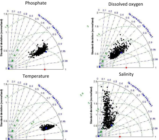
Figure 2 plots Taylor diagrams for the model-data comparison between the EFPC ensemble and observation fields for four oceanic properties: dissolved phosphate, dis-solved oxygen, temperature and salinity. The diagrams depict the relative performance
20
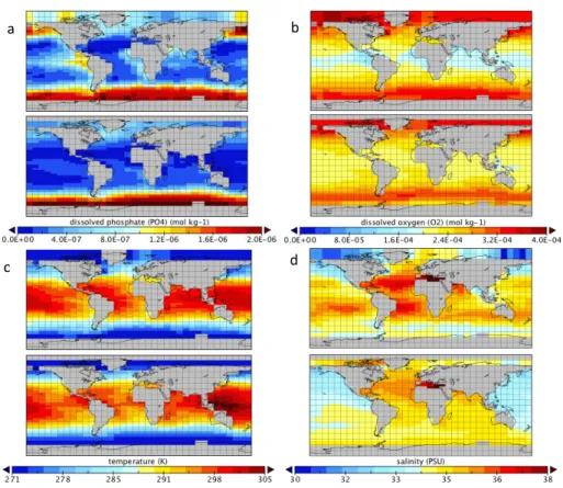
of the 471 ensemble members as well as the outputs of an optimised biogeochemi-cal configuration (Ridgwell and Death, 2012) for comparison. Figures 3 and 4 illustrate surface fields and latitude-depth transects through the Atlantic (25◦W) for the same
properties, in each case comparing observations with EFPC ensemble averages. Ob-served surface fields are depth-averages over the vertical extent of the surface layer of
25
BGD
9, 11843–11883, 2012
Controls on the spatial distribution of
oceanicδ13C DIC
P. B. Holden et al.
Title Page
Abstract Introduction
Conclusions References
Tables Figures
◭ ◮
◭ ◮
Back Close
Full Screen / Esc
Printer-friendly Version
Interactive Discussion
Discussion
P
a
per
|
Dis
cussion
P
a
per
|
Discussion
P
a
per
|
Discussio
n
P
a
per
|
5.1 Dissolved phosphate
The ensemble-averaged correlation of dissolved phosphate with respect to observa-tions (Garcia et al., 2006) is +0.88, compared to the optimised model correlation of +0.91. The ensemble-averaged variability of the spatial distribution captures the vari-ability of the observations more closely than the optimised model (the cloud is
ap-5
proximately centred on a normalised standard deviation of 1). These statistics together suggest that the neglect of the maximum phosphate uptake as a variable parameter has not biased the ability of the ensemble to capture a wide range of phosphate distri-butions that are consistent with observations. The ensemble-averaged surface field of dissolved phosphate compares reasonably with observations, although the increased
10
concentrations associated with upwelling regions are not well captured so that phos-phate is near-fully utilised throughout low and mid latitude oceans. Only 20 simulations exhibit surface-layer averaged phosphate concentrations that exceed observation es-timates of 0.6 µmol kg−1. The Atlantic cross-section compares favourably with obser-vations, although the volume and northerly extent of AABW are overestimated in the
15
ensemble average. This may be a consequence of the very high sea-ice diffusivities (SID) that have been allowed in the ensemble leading to increased brine rejection and AABW production. The EFPC distribution for SID is 52 000+/−26 000 m2s−1(1σ
un-certainties are quoted throughout). Previous studies that have generally not considered values above 25 000 m2s−1(e.g. Edwards et al., 2011).
20
5.2 Dissolved oxygen
Dissolved oxygen exhibits an ensemble-averaged correlation of +0.76 (c.f. +0.83 in the optimised model) and the normalised standard deviation is approximately centred on unity, demonstrating a comparable spatial variability to observations (Garcia et. al., 2006). The major weakness of the surface distribution reflects the weaknesses of the
25
BGD
9, 11843–11883, 2012
Controls on the spatial distribution of
oceanicδ13C DIC
P. B. Holden et al.
Title Page
Abstract Introduction
Conclusions References
Tables Figures
◭ ◮
◭ ◮
Back Close
Full Screen / Esc
Printer-friendly Version
Interactive Discussion
Discussion
P
a
per
|
Dis
cussion
P
a
per
|
Discussion
P
a
per
|
Discussio
n
P
a
per
|
to observations, a conspicuous difference being a∼20 % underestimate of oxygen in
NADW which, in the absence of large differences in temperature (Sect. 5.3 below), is suggestive of excess productivity in high northern latitudes and consistent with the underestimate of surface phosphate in the Arctic (Fig. 3). It could also reflect a bias towards low rates of air-sea gas exchange (see: Sect. 7), preventing the N. Atlantic
5
surface from fully equilibrating with the atmosphere. The plausibility constraints require reasonable globally averaged oxygen concentrations (∼170 µmol kg−1). It appears that
the underestimate of equatorial productivity, which we interpret as caused by a struc-tural issue, which cannot be addressed through the varied parameters, may have been compensated for by favouring parameters that compensate by increasing productivity
10
in high latitudes, notably high northern latitudes that are not Fe-limited.
5.3 Temperature
Temperature exhibits an ensemble-averaged correlation with observations (Locarnini et al., 2006) of+0.96, comparable to the optimised model. The spatial variability tends to be greater than observations, a feature which is shared with the optimised model.
15
The ensemble-averaged SST field agrees very well with observations, so that the overestimate of spatial variability is not reflected in this layer. The ensemble-averaged equator-to-pole SST temperature gradient reflects observations closely, important here given the strong temperature dependence of carbon isotope fractionation during air-sea gas exchange (Mook, 1986). The overestimate of the spatial variance is rather related
20
to the vertical temperature gradient (Fig. 4), which is greater than observations. This is likely, at least in part, a further consequence of the excessive strength of the AABW cell in the ensemble average.
5.4 Salinity
The ensemble-averaged salinity correlation with observations (Antonov et al., 2006)
25
BGD
9, 11843–11883, 2012
Controls on the spatial distribution of
oceanicδ13C DIC
P. B. Holden et al.
Title Page
Abstract Introduction
Conclusions References
Tables Figures
◭ ◮
◭ ◮
Back Close
Full Screen / Esc
Printer-friendly Version
Interactive Discussion
Discussion
P
a
per
|
Dis
cussion
P
a
per
|
Discussion
P
a
per
|
Discussio
n
P
a
per
|
as atmospheric moisture transport in the simple EMBM is dominated by diffusion. In the Bern3D model (structurally very similar to the configuration of GENIE used here as both are based on the same progenitor ocean model), optimised salinity corre-lations of 0.65 were obtained (Ritz et al., 2011), compared to 0.9 when the ocean model was restored to climatological sea-surface temperature and salinity fields (M ¨uller
5
et al., 2006). The salinity correlation across the EPFC ensemble (i.e. the correlation displayed separately by each of the 471 simulated fields with observations) exhibits a correlation of 0.54 with the atmospheric moisture diffusivity parameter (AMD). Low atmospheric diffusivity inhibits moisture transport out of low latitudes, restricting the de-velopment of the increased surface salinities that are observed there. EPFC-averaged
10
AMD of 8.4×10⁵m2s−1 is somewhat low compared to optimised values ranging
be-tween∼1×10⁶and 3×10⁶m2s−1 (Lenton et al., 2006). We note that the sign of the
vertical salinity gradient in the Pacific can be reversed due to this effect resulting in the very low correlations that are seen in some ensemble members.
An important decision therefore was whether to apply additional filters to the EPFC
15
ensemble in order to eliminate those simulations with poorly correlated salinity fields. Outside of the Arctic, the spatial pattern of the ensemble mean surface salinity is rea-sonable, although it exhibits a bias of∼ −1 psu (Fig. 3). We note that the ensemble
vari-ability of Atlantic (Pacific) surface salinity varies spatially from∼0.2 to 0.4 psu (∼0.5
to 1 psu). The salinity latitude-depth cross-sections in the Atlantic compare
reason-20
ably with observations (Fig. 4), though again they exhibit a low bias. The major dis-agreement is thus the understated surface salinities at low to mid latitudes, which may have important consequences for biological production via impacts on stratification-dependent mixing and the redistribution of nutrients back to the photic zone. To test for this, a salinity-correlation filter was applied to leave only the 112 ensemble members
25
with a salinity correlation>0.6. The cross-sections of 112-member ensemble-averaged phosphate, oxygen andδ13CDIC in the Atlantic, Pacific and Indian oceans were very
BGD
9, 11843–11883, 2012
Controls on the spatial distribution of
oceanicδ13C DIC
P. B. Holden et al.
Title Page
Abstract Introduction
Conclusions References
Tables Figures
◭ ◮
◭ ◮
Back Close
Full Screen / Esc
Printer-friendly Version
Interactive Discussion
Discussion
P
a
per
|
Dis
cussion
P
a
per
|
Discussion
P
a
per
|
Discussio
n
P
a
per
|
philosophy of the ensemble design. To illustrate, a comparison of theδ13CDIC
cross-sections of the means of the two ensembles exhibits anR2of>99 % in all three basins, although the salinity-filtered ensemble exhibits a slightly elevated average δ13CDIC
(0.89 ‰ c.f. 0.85 ‰ in the Atlantic, 0.40 ‰ c.f. 0.23 ‰ in the Pacific and 0.61 ‰ c.f. 0.55 ‰ in the Indian Oceans). We decided to retain all 471 of the EFPC members,
5
anticipating that the benefits of a large ensemble likely outweigh any beneficial effects of applying this filter.
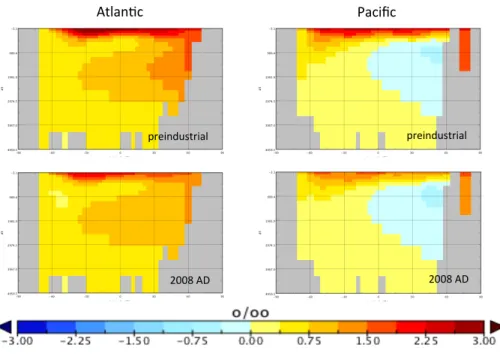
5.5 Oceanδ13CDIC
Figure 5 shows EPFC pre-industrial and modern (2008 AD) ensemble-averaged latitude-depth transects ofδ13CDIC through the Atlantic (25◦W) and Pacific (155◦W).
10
The discussion in the following paragraphs addresses the evaluation of the simulated present day δ13CDIC distribution with respect to the observational data of Kroopnick (1985, Figs. 3 and 5 therein) and Gruber et al. (1999).
In the Atlantic, ensemble-averagedδ13CDIC of AABW and AAIW masses varies in
the range ∼0.3 ‰ to ∼0.7 ‰ and NADW varies in the range ∼0.7 ‰ to ∼1.2 ‰,
15
in both cases consistent with observations (Kroopnick, 1985). The simulated 0.75 ‰ contour extends to∼35◦S, again in good agreement with the observational data, but
only reaches depths of∼3000 m, in disagreement with the observations, which
indi-cate that values in excess of 0.7 ‰ extend to the ocean floor north of the Equator. This is consistent with the excessive northerly penetration of AABW that is apparent
20
in the phosphate distribution (Sect. 5.1). We note that ensemble-averaged oceanic-meanδ13CDIC=0.38+/−0.22 ‰ is slightly lower than observational estimates of 0.5 ‰
(Quay et al., 2003), also consistent with too much simulated AABW.
In the Pacific, ensemble averaged δ13CDIC at depths below 1000 m ranges from
∼ −0.5 ‰ at high northern latitudes to∼0.4 ‰ at high southern latitudes. These are in
25
BGD
9, 11843–11883, 2012
Controls on the spatial distribution of
oceanicδ13C DIC
P. B. Holden et al.
Title Page
Abstract Introduction
Conclusions References
Tables Figures
◭ ◮
◭ ◮
Back Close
Full Screen / Esc
Printer-friendly Version
Interactive Discussion
Discussion
P
a
per
|
Dis
cussion
P
a
per
|
Discussion
P
a
per
|
Discussio
n
P
a
per
|
as low as−1.0 ‰ at high northern latitudes. In the simulations, the 0 ‰ contour extends
south to∼10◦S and to depths of∼3000 m, in good agreement with observations.
Simulated surface values of δ13CDIC in the Pacific of ∼1.5 ‰ are ∼0.3 ‰ lower
than observations of Gruber et al. (1999), consistent with a 13C Suess effect of
−0.018 ‰ yr−1 (Gruber et al., 1999). Simulated Atlantic surface δ13CDIC of ∼2 ‰ is
5
comparable to Gruber et al. (1999), so that the lack of a “Suess-offset” indicates a high-bias (∼0.3 ‰) in simulations of surface Atlanticδ13CDIC. Meridional surface profiles
dis-play similar characteristics to observations of Gruber et al. (1999): low values (∼1 ‰)
at high southern latitudes of the Atlantic, a maximum in both basins at∼40◦S to 50◦S,
a peak in the Pacific at∼15◦S and a trough in the Atlantic at∼30◦N (located at∼20◦N
10
in the simulations). These complex surface distributions can be explained through the interplay of the temperature-dependent fractionation of air-sea exchange, upwelling of
13
C depleted waters in the Southern Ocean and meridionally variable biological up-take rates and fractionation, greatest in regions of nutrient upwelling and lowest in the centres of sub-tropical gyres (Gruber et al., 1999).
15
6 Drivers of the spatial distribution of pre-industrialδ13CDIC
Aside from the excessive northerly intrusion of AABW and the ∼0.3 ‰ high-bias in
surface Atlantic δ13CDIC, the ensemble-averaged δ 13
CDIC spatial distributions are in
good agreement with the observations of Kroopnick (1985) and Gruber et al. (1999). The following analysis seeks to explain the processes and parameters that determine
20
the spatial distributions. We apply singular vector decomposition (SVD) to determine the dominant patterns (empirical orthogonal functions, EOFs) of variability across the ensemble and then to emulate the principal components (PCs) as functions of model parameters. Any of the simulated fields can be constructed as a linear combination of EOFs, weighted by their respective PCs. As such, an emulation of a PC can be used
25
BGD
9, 11843–11883, 2012
Controls on the spatial distribution of
oceanicδ13C DIC
P. B. Holden et al.
Title Page
Abstract Introduction
Conclusions References
Tables Figures
◭ ◮
◭ ◮
Back Close
Full Screen / Esc
Printer-friendly Version
Interactive Discussion
Discussion
P
a
per
|
Dis
cussion
P
a
per
|
Discussion
P
a
per
|
Discussio
n
P
a
per
|
anomaly (the difference between years 2008 and 1858) in order to separate equilibrium effects from the13C Suess effect.
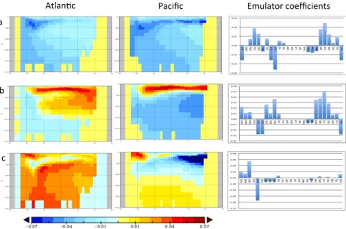
6.1 EOF decomposition
We consider two latitude-depth transects through the Atlantic (25◦W) and Pacific (155◦W). These transects run between latitudes 71◦S and 63◦N, thus including the
5
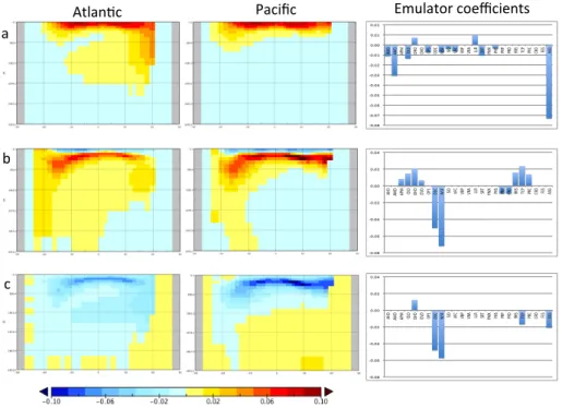
Southern Ocean but not the Arctic Ocean. The EFPC ensemble was decomposed into EOFs by applying SVD to the centred fields (i.e. after subtracting the ensemble mean). The SVD was applied to a single column vector constructed from the combined Atlantic and Pacific fields in order to derive a single set of EOFs that consistently de-scribes both basins. Figure 6 shows the first three EOFs, plotted separately in the two
10
basins. These three EOFs explain 42 %, 27 % and 11 % of the variance across the ensemble. Figure 6 additionally shows the emulator coefficients associated with each EOF, discussed in Sect. 6.2.
The first EOF is of the same sign (negative) at every location across the two basins, suggesting that this EOF relates primarily to a global-scale change in oceanicδ13CDIC.
15
This change is not uniformly distributed throughout the global ocean, but is qualita-tively similar to the spatial pattern of the ensemble mean in both basins (Fig. 5). The correlation between globally averagedδ13CDICand the 1st PC is−0.93, confirming this
interpretation. (Note that both the EOF and the correlation coefficient have a negative sign.) The change in globally averagedδ13CDICis dominantly associated with changes
20
in theδ13CDIC of AABW and AAIW. The Pacific EOF (average−0.035) has a greater
magnitude than the Atlantic EOF (−0.026) so, volume effects aside, a global increase
inδ13CDIC appears to be more pronounced in the Pacific Ocean, reflecting the
addi-tional influence of Antarctic water masses in this basin. Note that changes in global
δ13CDICare a result of surface restoring (as atmospheric concentrations are relaxed to
25
BGD
9, 11843–11883, 2012
Controls on the spatial distribution of
oceanicδ13C DIC
P. B. Holden et al.
Title Page
Abstract Introduction
Conclusions References
Tables Figures
◭ ◮
◭ ◮
Back Close
Full Screen / Esc
Printer-friendly Version
Interactive Discussion
Discussion
P
a
per
|
Dis
cussion
P
a
per
|
Discussion
P
a
per
|
Discussio
n
P
a
per
|
The second EOF does not exhibit a constant sign, but rather reflects a change in the spatial distribution ofδ13CDIC. In the Pacific, the EOF clearly reflects the variability in
the exchange of δ13CDIC values between surface and deep water (i.e. via the export
of particulate organic carbon POC). This interpretation also appears to be valid for the Atlantic, especially given that these two fields are from a single EOF and so should
5
reflect modes of variability that are closely related. The Atlantic EOF is complicated by the fact that changes in the surfaceδ13CDICare transmitted to NADW, so that increased POC export results in elevatedδ13CDICin both surface waters and NADW. Whilst the
basin-wide average of the second EOF in the Atlantic is of positive sign, in the Pacific it is negative, suggesting that some of the light carbon exported from the surface waters
10
of the Atlantic ends up in the deep Pacific. The second PC exhibits a correlation of
−0.30 with global POC export, so as POC export increases the vertical gradient of δ13CDICis reduced. This is discussed further in Sect. 6.2. Furthermore, the second PC exhibits a weak correlation (+0.2) with the globally-averaged DIC inventory, so that an increase in the DIC reservoir is associated with an increase in the vertical gradient of
15
δ13CDIC, consistent with the application of this metric as a proxy for oceanic carbon storage and atmospheric CO2(Shackleton et al., 1983).
The third EOF takes generally positive values throughout the Atlantic and generally negative values throughout the Pacific, suggesting it describes a mechanism for inter-basin exchange of δ13CDIC. The greatest variability in the Atlantic is apparent at the
20
boundary between Atlantic and Antarctic source waters, suggesting that this EOF re-flects the relative influence of these water masses. Increased influence of NADW leads to increased values of deep Atlanticδ3CDIC. This may be associated with a depletion
of13CDICin the Arctic Ocean that possibly explains the loweredδ 13
CDICin the surface
waters of the Northern Pacific (connected, in this model configuration, via diffusive
25
BGD
9, 11843–11883, 2012
Controls on the spatial distribution of
oceanicδ13C DIC
P. B. Holden et al.
Title Page
Abstract Introduction
Conclusions References
Tables Figures
◭ ◮
◭ ◮
Back Close
Full Screen / Esc
Printer-friendly Version
Interactive Discussion
Discussion
P
a
per
|
Dis
cussion
P
a
per
|
Discussion
P
a
per
|
Discussio
n
P
a
per
|
6.2 Principal component emulation
In order to better understand which parameters, and hence which processes, are driv-ing the spatial variability in simulatedδ13CDIC, simple linear emulators of the first three
PCs corresponding to the EOFs described in Sect. 6.1 were derived.
ζ(θ)=a+
n
X
i=1
biθi (1)
5
where each PCζ is expressed in terms of the 25 parametersθi and the scalar coeffi -cientsaandbi. Note that not all possible terms are included as the function is required
to satisfy the Bayes Information Criterion. Linear terms were found sufficient to pro-duce models with an adequate fit (modelR2∼85 % in each of the three PC models)
and are more straightforward to interpret than more complex (e.g. quadratic) functions.
10
Strong correlations exist between many parameter pairs; twelve parameter pairs ex-hibit a correlation (positive or negative) of >0.3. These correlations were introduced by the ensemble design (which constrains for plausible pre-industrial states) and their presence makes cross-terms difficult to reliably interpret. The parameter coefficientsbi
for each of the PC emulators are plotted in Fig. 6.
15
In Sect. 6.1, the 1st EOF was identified as corresponding to changes in globally averaged δ13CDIC. Parameters that are positively correlated with the global δ
13
CDIC
(negatively correlated with the 1st PC) are wind-stress scaling (WSF, via surface layer mixing, leading to co-varying productivity and POC export), atmospheric heat diff u-sivity AHD (modulating the equator-pole temperature gradient), overall air-sea gas
20
exchange strength (ASG) and ocean frictional drag (ODC). Increases in either the rain-ratio scalar (RRS) or the thermodynamic calcification rate power (TCP) act to de-crease globalδ13CDIC(increasing the export of CaCO3at the expense of POC export).
Increases in OL0 act to warm the surface ocean by decreasing outgoing longwave radiation, decreasing global δ13CDIC via temperature fractionation during air-sea gas
25
BGD
9, 11843–11883, 2012
Controls on the spatial distribution of
oceanicδ13C DIC
P. B. Holden et al.
Title Page
Abstract Introduction
Conclusions References
Tables Figures
◭ ◮
◭ ◮
Back Close
Full Screen / Esc
Printer-friendly Version
Interactive Discussion
Discussion
P
a
per
|
Dis
cussion
P
a
per
|
Discussion
P
a
per
|
Discussio
n
P
a
per
|
and increased globalδ13CDIC. Ocean-meanδ 13
CDICacross the ensemble satisfies the
relationshipδ13CDIC=−0.091T+2.159 (R2=21 %), where T is the globally average
sea-surface temperature, consistent with the temperature variation of oceanic δ13C in thermodynamic equilibrium with atmospheric δ13C of CO2 of −0.1 ‰◦C−
1
(Mook, 1986).
5
The second PC appears to be mainly controlled by ocean diffusivities, wind stress scaling and by particulate export, remineralisation and air-sea gas exchange. This sup-ports the inference that the second EOF describes the variability of exchange of carbon between the surface and deep ocean. The remineralisation depth (PRD) and the rain-ratio parameters (RRS and TCP) are all negatively correlated with export production.
10
Increases in these parameters lead to the transfer of nutrients to deeper depths from where they cannot be re-mixed or upwelled as readily into the euphotic zone. This en-hanced export of nutrients to depth thus decreases productivity so that an increase in these parameters results in increased near-surface values ofδ13CDIC.
The third PC clearly appears to be most strongly determined by isopycnal diffusivity
15
OHD. This parameter correlates strongly with the strength of the AABW cell (+0.37), so that high values of OHD are associated with strengthened AABW circulation (within which DIC is depleted inδ13CDIC relative to NADW). Conversely, high values of APM, the other major determinant of the third PC, lead to strengthening of NADW (through a reduction in Atlantic surface salinity) and relative enrichment ofδ13CDICin the region
20
where the boundaries between NADW and AABW are least clearly defined across the ensemble. As noted in Sect. 6.1, this effect appears to dominantly control the inter-basin contrast ofδ13CDIC, although the third PC is weakly correlated with the global
averageδ13C (+0.09), suggesting it is also associated with an effect on the oceanic-mean ofδ13CDIC. Note that the three PCs together explain 99.4 % of the variance in
25
the ocean-mean δ13CDIC, (86.0 %, 12.5 % and 0.9 % respectively) so that almost all of the ensemble variability in ocean-mean pre-industrialδ13CDICis described by these
BGD
9, 11843–11883, 2012
Controls on the spatial distribution of
oceanicδ13C DIC
P. B. Holden et al.
Title Page
Abstract Introduction
Conclusions References
Tables Figures
◭ ◮
◭ ◮
Back Close
Full Screen / Esc
Printer-friendly Version
Interactive Discussion
Discussion
P
a
per
|
Dis
cussion
P
a
per
|
Discussion
P
a
per
|
Discussio
n
P
a
per
|
7 Decomposition and emulation of the industrial13C imprint
The method presented in Sect. 6 has been re-applied here to explore the change in theδ13CDICdistribution from pre-industrial to modern times. The EOF analysis and PC
emulation is now applied to investigate the processes and parameters controlling the transient response to changes in the atmospheric carbon dioxide concentrations and
5
its isotopic composition. We restrict our analysis to the first two EOFs, which describe 63 % and 18 % of the variance of the transient response, respectively. The Atlantic and Pacific EOFs, together with the parameters in the linear emulator (Eq. 1) are plotted in the upper two panels of Fig. 7.
The first EOF is of constant sign throughout both basins and so represents a change
10
in global δ13CDIC. This can be interpreted as simply due to the uptake of relatively light carbon from the atmosphere (in which the13C-isotopic ratio has moved to lower values since pre-industrial times as a result of the burning of isotopically light fossil fu-els). This change is restricted to depths up to∼1000 m in the Pacific, but the changes
are redistributed to greater depth by NADW in the Atlantic. Unsurprisingly, the first PC
15
emulator is dominated by the air-sea gas exchange parameter, which exhibits a cor-relation of−0.89 with the first PC. Globally increasing air-sea gas exchange strength
acts to reduce the equilibration timescale of surface δ13CDIC with atmospheric δ 13
C. (The negative correlation is consistent with a lowering of the δ13CDIC as the EOF is
of positive sign.) The equilibration timescale forδ13CDIC at the sea surface is of the
20
order of a decade, hence there are large disequilibria at the air sea interface (see e.g. Gruber et al., 1999). In this regard, we note that the air-sea gas exchange pa-rameterisation (following Wanninkhof, 1992) is proportional to the square of the wind speed, but is applied to the long-term average wind-speed, thus neglecting non-linear contributions of short-term variability which contribute substantially to the globally
av-25
BGD
9, 11843–11883, 2012
Controls on the spatial distribution of
oceanicδ13C DIC
P. B. Holden et al.
Title Page
Abstract Introduction
Conclusions References
Tables Figures
◭ ◮
◭ ◮
Back Close
Full Screen / Esc
Printer-friendly Version
Interactive Discussion
Discussion
P
a
per
|
Dis
cussion
P
a
per
|
Discussion
P
a
per
|
Discussio
n
P
a
per
|
Further to this, a model error was recently discovered that introduces an artificial un-derestimation of the wind speed in some grid cells close to continental boundaries. The wide range over which the air-sea gas exchange was varied is likely to compensate for these shortcomings on the global scale. The ensemble-average of the global mean gas exchange coefficient for CO2of 0.038+/−0.14 mol m−2yr−1µatm−1 compares to the
5
range of (0.052+/−0.010) mol m−2yr−1µatm−1, based on the estimate of the air-sea
gas exchange velocity (and an estimate of the globally-averaged solubility of CO2) by
Naegler (2009). Thus, while the ASG parameter (0.1 to 0.5) spans the value for long-term average wind-speeds (0.39), given by Wanninkhof (1992), our central estimate for the global mean gas exchange coefficient is on the low side, which may reflect the
10
information about fluctuating wind direction that is lost in calculating annually-averaged wind stress (from which wind speed is subsequently derived).
The second EOF describes the partitioning ofδ13CDICbetween surface and
interme-diate waters, indicative of the degree to which the isotopically-lightened surface carbon is mixed with intermediate waters. The linear emulator of the second PC is dominated
15
by the global wind-stress scaling factor and the ocean drag coefficient. High values of either parameter increase mixing and upwelling, resulting in preferential lowering of
δ13CDICin intermediate waters relative to surface waters.
A similar analysis was performed for the anthropogenic change in DIC. The first EOF and the emulator coefficients for the change in DIC are plotted in Fig. 7. The
dom-20
inant mode of DIC variability (54 % of the ensemble variance) is strikingly similar to the second EOF of the industrial change inδ13CDIC. Furthermore, the corresponding
PC emulators exhibit similar dependencies on model parameters, negatively correlated with the ocean drag (ODC) and wind-scaling (WSF), suggesting a close physical rela-tionship between these modes of variability. The dominant mode of 13C Suess-effect
25
BGD
9, 11843–11883, 2012
Controls on the spatial distribution of
oceanicδ13C DIC
P. B. Holden et al.
Title Page
Abstract Introduction
Conclusions References
Tables Figures
◭ ◮
◭ ◮
Back Close
Full Screen / Esc
Printer-friendly Version
Interactive Discussion
Discussion
P
a
per
|
Dis
cussion
P
a
per
|
Discussion
P
a
per
|
Discussio
n
P
a
per
|
8 Summary and conclusions
We have described the development and evaluation of a large ensemble of precali-brated parameterisations of GENIE for application to coupled carbon cycle problems. These parameterisations have already been applied to a range of experiments (Eby et al., 2012; Holden et al., 2012; Joos et al., 2012; Zickfeld et al., 2012). Work is
5
presently in progress to apply them to a transient ensemble of simulations over the most recent glacial cycle, an experiment that has the potential to be constrained by a rich compilation of water-columnδ13CDICreconstructions from marine sediment data
(e.g. Oliver et al., 2010).
We have applied singular vector decomposition and principal component emulation
10
(Holden and Edwards, 2010) to investigate the modes of ensemble variability of the oceanic distribution ofδ13CDIC, considering both the pre-industrial state and the
tran-sient changes due to the Suess Effect. These analyses allow us to separate the natural and anthropogenic controls on the δ13CDIC distribution. The two analyses are
con-nected by the possibility for compensating errors in the two distributions when
mod-15
elling the modern ocean. For example, the second-order mode of variability in the preindustrial state (second EOF, Fig. 6) has a similar spatial distribution to the dom-inant mode of variability due to the Seuss effect (first EOF, Fig. 7), although they are controlled by quite distinct process (surface-deep ocean exchange and air-sea gas exchange, respectively).
20
The analysis provides a quantitative demonstration of the well-known balance be-tween physical and biogeochemical processes that control the vertical gradient of
δ13CDIC (Tagliabue and Bopp, 2008). These same controls exert an influence on the
global DIC inventory in the equilibrium state (as distinct from change in the inven-tory due to anthropogenic forcing), supporting the use of the surface-deep gradient as
25
a proxy for past ocean productivity-driven changes in atmospheric CO2 (Shackleton
BGD
9, 11843–11883, 2012
Controls on the spatial distribution of
oceanicδ13C DIC
P. B. Holden et al.
Title Page
Abstract Introduction
Conclusions References
Tables Figures
◭ ◮
◭ ◮
Back Close
Full Screen / Esc
Printer-friendly Version
Interactive Discussion
Discussion
P
a
per
|
Dis
cussion
P
a
per
|
Discussion
P
a
per
|
Discussio
n
P
a
per
|
Uncertainty in the distribution ofδ13CDICdue to the Suess effect is dominated by
air-sea gas exchange. The first EOF describes 63 % of the variability across the ensemble and is controlled almost entirely by the air-sea gas exchange parameter. The second EOF, describing 18 % of the variance, is driven by uncertainties in ocean parameters that control mixing of intermediate and surface waters. However, the decomposition
5
of the distribution of anthropogenic DIC demonstrates, unsurprisingly, that air-sea gas exchange does not contribute substantially to uncertainty in the ocean carbon-sink. Rather, the dominant mode of variability (54 %) is strikingly similar to the second order variability in the Suess effect. Furthermore these two modes of variability are controlled by the same parameter relationships and hence, presumably, by the same physical
pro-10
cesses. This comparison highlights well-known complications that arise when applying
δ13CDICas a constraint on the ocean sink and the need to separate the effects of uncer-tainty due to air-sea gas exchange. However, the similarity of the modes of variability of DIC andδ13CDICafter removal of the air-sea gas imprint strongly supports the value of
observationally-based constraints imposed byδ13CDICon DIC uptake (e.g. Quay et al.,
15
2003). (Note these methodologies correct for the air-sea gas exchange signal). The need for a precise separation of the influence of air-sea gas exchange suggests that improved observational coverage ofδ13CDICis essential for improved quantification of the ocean-sink.
Acknowledgements. PBH and NRE acknowledge support from EU FP7 ERMITAGE grant
20
BGD
9, 11843–11883, 2012
Controls on the spatial distribution of
oceanicδ13C DIC
P. B. Holden et al.
Title Page
Abstract Introduction
Conclusions References
Tables Figures
◭ ◮
◭ ◮
Back Close
Full Screen / Esc
Printer-friendly Version
Interactive Discussion
Discussion
P
a
per
|
Dis
cussion
P
a
per
|
Discussion
P
a
per
|
Discussio
n
P
a
per
|
References
Annan, J. D. and Hargreaves, J. C.: Efficient identification of ocean thermodynamics in a
phys-ical/biogeochemical ocean model with an Iterative Importance Sampling Method, Ocean Model., 32, 205–215, doi:10.1016/j.ocemod.2010.02.003, 2010.
Antonov, J. I., Locarnini, R. A., Boyer, T. P., Mishonov, A. V., and Garcia, H. E.: World Ocean
At-5
las 2005, Volume 2, edited by: Salinity. S., Levitus, NOAA Atlas NESDIS 62, US Government
Printing Office, Washington, D.C., 182 pp., 2006.
Archer, D.: A data-driven model of the global calcite lysocline, Global Biogeochem. Cy., 10, 511–526, doi:10.1029/96GB01521, 1996.
Bondeau, A., Smith, P. C., Zaehle, S., Schaphoff, S., Lucht, W., Cramer, W., Gerten, D.,
Lotze-10
Campen, H., M ¨uller, C., Reichstein, M., and Smith, B.: Modelling the role of agriculture for the 20th century global terrestrial carbon balance, Glob. Change Biol., 13, 679–706, doi:doi:10.1111/j.1365-2486.2006.01305.x, 2007.
Bouttes, N., Paillard, D., and Roche, D. M.: Impact of brine-induced stratification on the glacial carbon cycle, Clim. Past, 6, 575–589, doi:10.5194/cp-6-575-2010, 2010.
15
Bouttes, N., Paillard, D., Roche, D. M., Brovkin, V., and Bopp L.: Last Glacial Maximum CO2and
δ13C successfully reconciled, Geophys. Res. Lett., 38, L02705, doi:10.1029/2010GL044499,
2011.
Cavalieri, D. J., Parkinson, C. L., and Yinnikov, K. Y.: 30-year satellite record reveals con-trasting Arctic and Antarctic decadal sea-ice variability, Geophys. Res. Lett., 30, 1970,
20
doi:10.1029/2003GL018031, 2003.
Chikamoto, M. O., Abe-Ouchi, A., Oka, A., Ohgaito, R., and Timmermann, A.: Quantifying the
ocean’s role in glacial CO2reductions, Clim. Past, 8, 545–563, doi:10.5194/cp-8-545-2012,
2012.
Colbourn, G.: Weathering effects on the carbon cycle in an Earth System Model, PhD thesis,
25
School of Environmental Sciences, University of East Anglia, http://ethos.bl.uk/OrderDetails.
do?uin=uk.bl.ethos.537151, 2011.
Conkright, M. E., Locarnini, R. A., Garcia, H. E., OBrien, T. D., Boyer, T. P., Stephens, C., and Antonov, J. I.: World Ocean Atlas 2001: Objective Analysis, Data, Statistics and Figures, CD-ROM Documentation, National Oceanographic Data Center, Silver Spring, MD, 2002.