ACPD
15, 19947–20011, 2015Development of an atmospheric N2O
isotopocule model
K. Ishijima et al.
Title Page
Abstract Introduction
Conclusions References
Tables Figures
◭ ◮
◭ ◮
Back Close
Full Screen / Esc
Printer-friendly Version
Interactive Discussion
Discussion
P
a
per
|
Discussion
P
a
per
|
Discussion
P
a
per
|
Discussion
P
a
per
|
Atmos. Chem. Phys. Discuss., 15, 19947–20011, 2015 www.atmos-chem-phys-discuss.net/15/19947/2015/ doi:10.5194/acpd-15-19947-2015
© Author(s) 2015. CC Attribution 3.0 License.
This discussion paper is/has been under review for the journal Atmospheric Chemistry and Physics (ACP). Please refer to the corresponding final paper in ACP if available.
Development of an atmospheric N
2
O
isotopocule model and optimization
procedure, and application to source
estimation
K. Ishijima1, M. Takigawa1, K. Sudo2,1, S. Toyoda3, N. Yoshida4,5, T. Röckmann6, J. Kaiser7, S. Aoki8, S. Morimoto8, S. Sugawara9, and T. Nakazawa8
1
Department of Environmental Geochemical Cycle Research, JAMSTEC, Yokohama, Japan
2
Graduate School of Environmental Studies, Nagoya University, Nagoya, Japan
3
Department of Environmental Science and Technology, Tokyo Institute of Technology, Yokohama, Japan
4
Department of Environmental Chemistry and Engineering, Tokyo Institute of Technology, Yokohama, Japan
5
Earth-Life Science Institute, Tokyo Institute of Technology, Tokyo, Japan
6
Institute for Marine and Atmospheric research Utrecht, Utrecht University, Utrecht, the Netherlands
7
ACPD
15, 19947–20011, 2015Development of an atmospheric N2O
isotopocule model
K. Ishijima et al.
Title Page
Abstract Introduction
Conclusions References
Tables Figures
◭ ◮
◭ ◮
Back Close
Full Screen / Esc
Printer-friendly Version
Interactive Discussion
Discussion
P
a
per
|
Discussion
P
a
per
|
Discussion
P
a
per
|
Discussion
P
a
per
|
8
Center for Atmospheric and Oceanic Studies, Tohoku University, Sendai, Japan
9
Miyagi University of Education, Sendai, Japan
Received: 31 May 2015 – Accepted: 29 June 2015 – Published: 22 July 2015
Correspondence to: K. Ishijima ([email protected])
ACPD
15, 19947–20011, 2015Development of an atmospheric N2O
isotopocule model
K. Ishijima et al.
Title Page
Abstract Introduction
Conclusions References
Tables Figures
◭ ◮
◭ ◮
Back Close
Full Screen / Esc
Printer-friendly Version
Interactive Discussion
Discussion
P
a
per
|
Discussion
P
a
per
|
Discussion
P
a
per
|
Discussion
P
a
per
|
Abstract
This paper presents the development of an atmospheric N2O isotopocule model based
on a chemistry-coupled atmospheric general circulation model (ACTM). We also de-scribe a simple method to optimize the model and present its use in estimating the isotopic signatures of surface sources at the hemispheric scale. Data obtained from
5
ground-based observations, measurements of firn air, and balloon and aircraft flights were used to optimize the long-term trends, interhemispheric gradients, and photolytic fractionation, respectively, in the model. This optimization successfully reproduced
re-alistic spatial and temporal variations of atmospheric N2O isotopocules throughout the
atmosphere from the surface to the stratosphere. The very small gradients
associ-10
ated with vertical profiles through the troposphere and the latitudinal and vertical dis-tributions within each hemisphere were also reasonably simulated. The results of the isotopic characterization of the global total sources were generally consistent with pre-vious one-box model estimates, indicating that the observed atmospheric trend is the dominant factor controlling the source isotopic signature. However, hemispheric
esti-15
mates were different from those generated by a previous two-box model study, mainly
due to the model accounting for the interhemispheric transport and latitudinal and
verti-cal distributions of tropospheric N2O isotopocules. Comparisons of time series of
atmo-spheric N2O isotopocule ratios between our model and observational data from several
laboratories revealed the need for a more systematic and elaborate intercalibration of
20
the standard scales used in N2O isotopic measurements in order to capture a more
complete and precise picture of the temporal and spatial variations in atmospheric
N2O isotopocule ratios. This study highlights the possibility that inverse estimation of
surface N2O fluxes, including the isotopic information as additional constraints, could
be realized.
ACPD
15, 19947–20011, 2015Development of an atmospheric N2O
isotopocule model
K. Ishijima et al.
Title Page
Abstract Introduction
Conclusions References
Tables Figures
◭ ◮
◭ ◮
Back Close
Full Screen / Esc
Printer-friendly Version
Interactive Discussion
Discussion
P
a
per
|
Discussion
P
a
per
|
Discussion
P
a
per
|
Discussion
P
a
per
|
1 Introduction
Nitrous oxide (N2O) is currently one of the most remarkable atmospheric components
of the Earth’s environment, being both a greenhouse gas with high radiative efficiency
(100 year global warming potential or global temperature change potential of 200–300; Ciais et al., 2013), as well as the most influential ozone depleting substance (ODS)
5
emitted during this century, when CFC emissions have been largely reduced
follow-ing the Montreal Protocol (Ravishankara et al., 2009). N2O was originally a natural gas
component that was shown (from ice core records) to have existed prehistorically in the atmosphere (Schilt et al., 2010), and was mainly produced as an intermediate product or by-product during microbial utilization of nitrogen compounds in soils or oceans.
10
Generated in this way on the Earth’s surface, N2O is chemically inert in the
tropo-sphere. However, in the stratosphere, N2O is decomposed by photolysis and reaction
with O(1D). The latter reaction is a source of nitric oxide (NO), which is a main player
for stratospheric ozone depletion.
Around the mid-19th century, as industrialization expanded, the atmospheric N2O
15
mole fraction began to increase, and this growth was further accelerated in the 20th century (Machida et al., 1995; MacFarling Meure et al., 2006) following the increase in
global population. This increase in N2O levels is thought to have been caused by the
use of synthetic nitrogen fertilizers developed during the industrialization of the agri-cultural sector. Through the application of nitrogen fertilizers onto crops, the amount of
20
nitrogen compounds available for microbes increased, and N2O production inevitably
increased in the soil. It would be difficult to quickly reduce nitrogen fertilizer use in
crop production (in order to reduce N2O emissions) if we continue to feed the rapidly
increasing global population. Thus, the increase in the atmospheric N2O mole
frac-tion has continued at a rate of around 0.5–0.8 nmol mol−1a−1 near the surface since
25
the 1980s (Ciais et al., 2013). Various N2O sources other than agricultural soils are
known, and the sum of their emissions (2.8 Tg a−1N equivalents) is considered to be
contri-ACPD
15, 19947–20011, 2015Development of an atmospheric N2O
isotopocule model
K. Ishijima et al.
Title Page
Abstract Introduction
Conclusions References
Tables Figures
◭ ◮
◭ ◮
Back Close
Full Screen / Esc
Printer-friendly Version
Interactive Discussion
Discussion
P
a
per
|
Discussion
P
a
per
|
Discussion
P
a
per
|
Discussion
P
a
per
|
bution from each source to the global total is still only poorly understood and there are large uncertainties in the estimates (Ciais et al., 2013). Emission estimates for individual source categories are mainly derived from bottom-up approaches that com-bine field flux measurements and statistical data (e.g., data on nitrogen fertilizer use
in a given region), but large spatiotemporal variations in the N2O flux exist at the site
5
to local scales. Consequently, it is difficult to make representative and accurate
emis-sion estimates for each source, and thus develop strategies to efficiently reduce N2O
emissions at global and national levels.
One approach to separating out the contributions from individual sources is the use of isotopically-substituted molecules, or, short, isotopocules (Kaiser and Röckmann,
10
2008). The isotopocule ratio of N2O is altered by various biogeochemical processes,
such as biogenic production and consumption in the source areas, and also by chem-ical processes in the atmosphere. The isotopic composition of the precursors is also
reflected to some degree in the resultant N2O. Therefore, it is thought that stable
iso-topocule ratios could be used to quantify the contribution from individual N2O sources.
15
There have been many studies of the isotopic signatures of various N2O sources and
sinks, but a unique isotopic value for each source with an adequately small uncertainty range remains elusive because of the complicated tangle of the precursor’s isotopic signatures and microbial process-driven isotopic fractionation (e.g., Kim and Craig, 1993; Rahn and Wahlen, 2000; Toyoda et al., 2011, 2015). There have also been
ex-20
perimental or theoretical studies of isotopic fractionation driven by photochemical loss reactions (e.g., Selwyn and Johnston, 1981; Kaiser et al., 2002, 2003a; Nanbu and Johnson, 2004; von Hessberg et al., 2004; Schmidt et al., 2011). This fractionation
generates large vertical gradients in N2O mole fraction and isotopocule ratios, which
decrease and increase, respectively, with increasing altitude in the stratosphere (e.g.,
25
ACPD
15, 19947–20011, 2015Development of an atmospheric N2O
isotopocule model
K. Ishijima et al.
Title Page
Abstract Introduction
Conclusions References
Tables Figures
◭ ◮
◭ ◮
Back Close
Full Screen / Esc
Printer-friendly Version
Interactive Discussion
Discussion
P
a
per
|
Discussion
P
a
per
|
Discussion
P
a
per
|
Discussion
P
a
per
|
Levin, 2005; Bernard et al., 2006; Ishijima et al., 2007), although some recent
stud-ies have discussed seasonal cycles or interhemispheric differences (Park et al., 2012;
Toyoda et al., 2013). These studies have revealed that the observed decreasing trends
of, for example, the major nitrogen and oxygen isotope ratios of N2O, are caused by
the continuous input of N2O into the troposphere from anthropogenic sources, which,
5
based on a top-down approach using a simple box model and observed data, are
esti-mated to be on average isotopically lighter than tropospheric N2O (Toyoda et al., 2015).
It is now necessary to progress to the next stage of integrating the knowledge ob-tained (as above), and to comprehensively validate this knowledge, in order to recon-sider how and what should be the focus of study in this field. Global three-dimensional
10
(3-D) modelling is considered a possible avenue for such research. There have
al-ready been some attempts at global N2O isotopocule modelling (McLinden et al.,
2003; Morgan et al., 2004; Liang and Yung, 2007), but existing models have a fixed
N2O mole fraction in the lower troposphere and no surface emissions, or are
some-times two-dimensional, and this is because they were developed mainly to examine
15
photochemistry-induced isotopocule fractionation in the stratosphere. On the other
hand, several studies have performed global N2O inverse modelling to estimate
re-gional fluxes (Hirsch et al., 2006; Huang et al., 2008; Thompson et al., 2014a; Saikawa
et al., 2014). The derived regional N2O emission estimates are generally reasonable,
predominantly because of recently improved observation networks incorporating flask
20
sampling and in situ measurements (e.g., Dlugokencky et al., 1994; Tohjima et al., 2000; Prinn et al., 2000; Ishijima et al., 2009). However, it is still thought that some of the uncertainty in inverse estimations is caused by poor simulation of the stratosphere–
troposphere exchange (STE), which brings stratospheric N2O-depleted air into the
tro-posphere and influences spatiotemporal variations in the tropospheric mole fraction. In
25
terms of isotopocules, the N2O thus introduced into the troposphere by STE is rich in
heavier isotopocules, as N2O is enriched in heavier isotopocules in the stratosphere
by photochemical loss processes; therefore, as discussed by Park et al. (2012),
frac-ACPD
15, 19947–20011, 2015Development of an atmospheric N2O
isotopocule model
K. Ishijima et al.
Title Page
Abstract Introduction
Conclusions References
Tables Figures
◭ ◮
◭ ◮
Back Close
Full Screen / Esc
Printer-friendly Version
Interactive Discussion
Discussion
P
a
per
|
Discussion
P
a
per
|
Discussion
P
a
per
|
Discussion
P
a
per
|
tions. Unfortunately, atmospheric N2O isotopocule measurements have not reached
the level required for such inverse modelling or STE studies in terms of measurement precision and number of stations. However, in the near future, when high-frequency and high-precision optical measurement systems capable of continuously monitoring
atmospheric N2O isotopocule ratios (e.g., Waechter et al., 2008) are improved and
5
become more widely available, global atmospheric N2O isotopocule models could be
essential to our understanding of observed results (e.g., see Rigby et al., 2012 for the case of methane). Therefore, in this study we present an outline of a newly developed
N2O isotopocule model that explicitly handles surface emissions, together with a simple
approach to optimizing the model’s photochemical fractionation and surface emissions
10
using several types of observational data.
2 N2O isotopocules
2.1 Notation for N2O isotopocules
In this study, we use the term “isotopocule”, which was first proposed by Kaiser and Röckmann (2008) and has also recently been adopted by Coplen (2011) to designate
15
isotopically substituted molecules. The term encompasses the terms “isotopologue”
(a molecule differing only in isotopic composition; e.g.,14N14N16O and14N14N18O) and
“isotopomer” (molecules having the same number of each isotopic atom but differing in
their positions; e.g.,14N15N16O and 15N14N16O). Individual N2O isotopocules are
dis-tinguished by their molecular formula. We consider the following four N2O isotopocules:
20
14
N14N16O, 14N15N16O, 15N14N16O, and 14N14N18O in this study, and the notation of
ACPD
15, 19947–20011, 2015Development of an atmospheric N2O
isotopocule model
K. Ishijima et al.
Title Page
Abstract Introduction
Conclusions References
Tables Figures
◭ ◮
◭ ◮
Back Close
Full Screen / Esc
Printer-friendly Version
Interactive Discussion
Discussion
P
a
per
|
Discussion
P
a
per
|
Discussion
P
a
per
|
Discussion
P
a
per
|
δ15Ni =15Risample/15Ristd−1, (i = bulk, αorβ) (1)
δ18O=18Rsample/18Rstd−1, (2)
15Rα
=14N15N16O
/14N14N16O
, (3)
15Rβ
=15
N14N16O
/14
N14N16O
, (4)
15Rbulk
= 15Rα+15Rβ
/2, (5)
5
18R
=14N14N18O
/14N14N16O
. (6)
We also use the15N site preference (hereafterδ15Nsp), which is defined as the diff
er-ence between the two nitrogen isotopomer deltas:
δ15Nsp=δ15Nα−δ15Nβ. (7)
We note that in some publications, a different notation for the N2O isotopomers was
10
used, following Brenninkmeijer and Röckmann (1999). In publications from this group,
δ15Nα is denoted2δ15N andδ15Nβ is denoted1δ15N. Hereafter, we use “isotopocule
deltas” as an inclusive term forδ15Nbulk,δ18O,δ15Nα,δ15Nβ, andδ15Nsp.
2.2 Conversion of isotopocule ratio to mole fraction
When we simulate N2O isotopocules in a model or use the observational data to
op-15
timize the model, the isotopocule ratios must be converted to the absolute mole
frac-tions. In this study, we calculated each isotopocule mole fraction assuming that N2O
consists of only four isotopocules:14N14N16O,14N15N16O,15N14N16O, and14N14N18O
as follows:
N2O
=14N14N16O
+14N15N16O
+15N14N16O
+14N14N18O
. (8)
20
By substituting Eqs. (3), (4), and (6) into Eq. (8), we have
14
N14N16O
=N2O
/ 1+15Rα+15Rβ+18R
ACPD
15, 19947–20011, 2015Development of an atmospheric N2O
isotopocule model
K. Ishijima et al.
Title Page
Abstract Introduction
Conclusions References
Tables Figures
◭ ◮
◭ ◮
Back Close
Full Screen / Esc
Printer-friendly Version
Interactive Discussion
Discussion
P
a
per
|
Discussion
P
a
per
|
Discussion
P
a
per
|
Discussion
P
a
per
|
As these four isotopocules account for more than 99.9 % of all of the atmospheric
N2O isotopocules, and assuming statistical isotope distributions for the three atoms in
the N2O molecule (x(14N14N16O)=99.01 %, x(14N15N16O)=0.37 %, x(15N14N16O)=
0.36 %, andx(14N14N18O)=0.21 %), neglecting less abundant species, will not
gener-ate any significant errors in the N2O isotopocule ratios finally obtained.
5
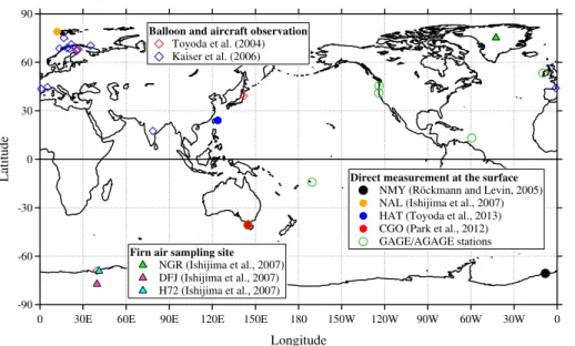
3 Observational data
We used three sets of observation data in the model optimization and analysis in this study. Table 1 and Fig. 1 summarize the details of the ground-based stations and the locations of all observations, respectively.
3.1 Time series data observed at a ground-based station
10
We used the high-precision N2O isotopocule ratio measurements of Röckmann and
Levin (2005). Air sampling was performed at the German Antarctic research station
Neumayer (71◦S, 8◦W, hereafter NMY) by the Alfred Wegener Institute for Polar
Re-search (AWI, Bremerhaven) since the early 1980s. From this dataset, twenty-three archived air samples for the period from March 1990 to November 2002 were
anal-15
ysed for N2O mole fraction at the University of Heidelberg (Schmidt et al., 2001)
us-ing ECD-GC (an Electoron Capture Detector equipped Gas Chromatography), based on a standard scale developed by The Advanced Global Atmospheric Gases Exper-iment (AGAGE), and also a high-precision isotopocule ratio measurement technique (Röckmann et al., 2005) for isotopocule ratios at the Max Planck Institute for
Nu-20
clear Physics (Heidelberg). This dataset shows highly stable temporal variations
(stan-dard error about 0.14 nmol mol−1, 0.01, 0.02, 0.07, and 0.06 ‰ for the mole fraction,
δ15Nbulk, δ18O, δ15Nα, andδ15Nβ, respectively) compared with other datasets (Park
et al., 2012; Toyoda et al., 2013), because the measurement precision was very high, and also the station is very close to being a true background site and so is less
ACPD
15, 19947–20011, 2015Development of an atmospheric N2O
isotopocule model
K. Ishijima et al.
Title Page
Abstract Introduction
Conclusions References
Tables Figures
◭ ◮
◭ ◮
Back Close
Full Screen / Esc
Printer-friendly Version
Interactive Discussion
Discussion
P
a
per
|
Discussion
P
a
per
|
Discussion
P
a
per
|
Discussion
P
a
per
|
fected by nearby sources. The advantage is obvious in comparison with other stations showing highly variable results and sometimes blurring the trends due to low measure-ment precisions and/or local source influences (Fig. 10). Consequently, this dataset
was considered suitable for the first step of developing an N2O isotopocule model with
simplified surface emissions of a spatiotemporally constant isotopocule ratio. In
Röck-5
mann and Levin (2005), results for δ15Nα and δ15Nβ are shown using two different
standard scales from the Max-Planck Institute (Kaiser et al., 2003b) and the Tokyo In-stitute of Technology (Toyoda and Yoshida, 1999), but we used the latter scale, which
has been supported by further reports (Griffith et al., 2009; Westley et al., 2007), for all
data in this study.
10
3.2 Time series data reconstructed from analysis of firn air obtained from the
polar ice sheets
We also used historical data of atmospheric N2O mole fraction and isotopocule ratios,
which were reconstructed from analysis of firn air samples obtained from three sta-tions in both the Arctic and Antarctic regions (Ishijima et al., 2007; Table 1; Fig. 1);
15
North GRIP (75◦N, 43◦W, 2959 m a.s.l., hereafter NGR), Greenland, Dome Fuji (77◦S,
40◦E, 3810 m a.s.l., hereafter DFJ) and H72 (69◦S, 41◦E, 1241 m a.s.l.), Antarctica.
Measurement precision (N2O: 0.3 nmol mol−1;δ15Nbulk: 0.1 ‰; δ18O: 0.2 ‰) was not
as high as the data from NMY, but only the decadal means of the record, which im-proves the standard error of the data, were used to limit the uncertainty in this study.
20
The standard scale was not adjusted to derive the interhemispheric differences,
be-cause all firn air samples were measured using a single analytical system with the same standard scale. Thus, we can ignore uncertainties caused by the standard scale
ACPD
15, 19947–20011, 2015Development of an atmospheric N2O
isotopocule model
K. Ishijima et al.
Title Page
Abstract Introduction
Conclusions References
Tables Figures
◭ ◮
◭ ◮
Back Close
Full Screen / Esc
Printer-friendly Version
Interactive Discussion
Discussion
P
a
per
|
Discussion
P
a
per
|
Discussion
P
a
per
|
Discussion
P
a
per
|
3.3 Vertical profile data in the stratosphere observed using balloon and aircraft
To validate the model for N2O mole fraction and isotopocule ratios in the stratosphere,
we used vertical profile data observed by balloons and aircraft between 1987 and 2007 (Toyoda et al., 2004; Kaiser et al., 2006). Toyoda et al. (2004) published balloon ob-servation data obtained until 2001, but unpublished data obtained by these authors
5
between 2002 and 2007 were also included in this study. Balloons were launched over locations in Sweden, France, India, Japan, and Antarctica (Fig. 1; detailed observation information in Toyoda et al., 2004; Kaiser et al., 2006), and 6 to 15 air samples were collected during each flight using a cryogenic sampler on board the balloon at altitudes of 10–35 km. Some aircraft observations from up to around 20 km height (Kaiser et al.,
10
2006), were also used in this study. Air samples were analysed for N2O mole
frac-tion and isotopic composifrac-tion in the laboratory. Measurement precisions (N2O<1 %;
δ15Nbulk and δ18O∼=0.5 ‰; δ15Nα and δ15Nβ<1.5 ‰) of the stratospheric samples
were relatively poor because of the limited volume of air sample taken, especially from higher altitudes, but were considered to be adequate considering the large vertical
15
gradients in the stratosphere.
4 Modelling
4.1 Model outline
We used the Center for Climate System Research/National Institute for Environmen-tal Stu-dies/Frontier Research Center for Global Change atmospheric general
circu-20
lation model (CCSR/NIES/FRCGC AGCM; Numaguti et al., 1997) with chemical
re-actions (which we refer to as the ACTM) to simulate atmospheric N2O isotopocules.
This model was described by Ishijima et al. (2010), but some improvements were
made to the chemistry–radiation calculations to better reproduce the stratospheric N2O
isotopocules (described below). The horizontal and vertical resolutions of the model
ACPD
15, 19947–20011, 2015Development of an atmospheric N2O
isotopocule model
K. Ishijima et al.
Title Page
Abstract Introduction
Conclusions References
Tables Figures
◭ ◮
◭ ◮
Back Close
Full Screen / Esc
Printer-friendly Version
Interactive Discussion
Discussion
P
a
per
|
Discussion
P
a
per
|
Discussion
P
a
per
|
Discussion
P
a
per
|
were T42 spectral truncation (about 2.8◦×2.8◦) and 67 sigma-pressure vertical layers
(surface to about 80 km), respectively. The model transport was nudged towards the Japanese 25 year ReAnalysis data by the Japan Meteorological Agency (JMA) (JRA-25; Onogi et al., 2007) for horizontal winds and temperature at 6 hly time intervals.
4.1.1 Stratospheric chemistry
5
The chemical loss of N2O by photolysis and two different oxidation reactions with O(1D)
in the stratosphere were incorporated into the model. Absorption cross-sections of N2O
and the oxidation reaction rate constants, which depend on the ultraviolet wavelength
and/or the air temperature, were taken from Sander et al. (2006). The N2O
photol-ysis rate (JN2O) was calculated for 15 bins from 178 to 200 nm (Schumann–Runge
10
bands) by a scheme (Akiyoshi et al., 2009) using the parameterization of Minschwaner et al. (1993), and for 3 bins from 200 to 278 nm by a main radiation–photolysis scheme of the ACTM (Sudo et al., 2002; Sekiguchi and Nakajima, 2008). The concentration
of O(1D) was calculated online in the ACTM using the prescribed ozone field, and
the photolysis of ozone was calculated for 9 bins from 200 to 355 nm. For the ozone
15
field, 6 hly full-resolution model level data from the ECMWF Interim Reanalysis (ERA-Interim, Dragani, 2011), and from Takigawa et al. (1999), were used up to and above 1 hPa, respectively.
4.1.2 Isotopocule fractionation
N2O isotopocule fractionation driven by photochemical reactions was incorporated
20
into the ACTM. We used the photolytic fractionation constants for 14N15N16O and
15
N14N16O of von Hessberg et al. (2004), which depend on both wavelength and
air temperature. We approximated the constant for 14N14N18O, as it was not
deter-mined by von Hessberg et al. (2004). We first calculated apparent fractionation
con-stants (hereafterεs), which are the slopes of the lines fitted to the Rayleigh plot of the
25
Toy-ACPD
15, 19947–20011, 2015Development of an atmospheric N2O
isotopocule model
K. Ishijima et al.
Title Page
Abstract Introduction
Conclusions References
Tables Figures
◭ ◮
◭ ◮
Back Close
Full Screen / Esc
Printer-friendly Version
Interactive Discussion
Discussion
P
a
per
|
Discussion
P
a
per
|
Discussion
P
a
per
|
Discussion
P
a
per
|
oda et al. (2004), and then interpolated the constants for14N15N16O and 15N14N16O
to obtain that of 14N14N18O so that the relationship of the εs of δ15Nα, δ15Nβ, and
δ18O was the same as that of the fractionation constants of 14N15N16O, 15N14N16O,
and 14N14N18O. However, these photolytic fractionations implemented in the model
were found to underestimate the observed εs, so we slightly modified the
fraction-5
ation in the model using a simple optimization method, as described in Sect. 4.2.3.
For oxidation with O(1D), we used the mean fractionation constants determined by
Kaiser et al. (2002), but we did not consider temperature dependence of the fractiona-tions, which are very small and thus do not contribute strongly to the fractionations in
the stratosphere compared to the photolytic fractionations. The four different species,
10
14
N14N16O, 14N15N16O, 15N14N16O, and 14N14N18O, are calculated separately in the
model.
4.1.3 Emission scenarios
We included the four source categories of N2O emissions in the model
simula-tions in this study; i.e., natural soils, oceans, anthropogenic, and biomass
burn-15
ing emissions. The annual mean natural soil emissions of N2O were taken from
the Emission Database for Global Atmospheric Research version 2 (EDGARv2; http://themasites.pbl.nl/tridion/en/themasites/edgar/emission_data/edgar2-1990). For oceanic emissions, the monthly varying emissions provided by Bouwman et al. (1995) (mostly based on Nevison et al., 1995) and Jin and Gruber (2003) were combined,
20
but scaled by 0.45 and 0.55, respectively. For anthropogenic emissions, we used the annual mean emissions from EDGARv4.2 (covering 1970–2000; http://edgar.jrc.ec. europa.eu) for 1984–1999, and from EDGARv4.2 FT2010 (covering 2000–2010) for 2000–2010, but the emissions from EDGARv4.2 were scaled so that the global to-tal emissions of each source category were consistent in 2000 between EDGARv4.2
25
ACPD
15, 19947–20011, 2015Development of an atmospheric N2O
isotopocule model
K. Ishijima et al.
Title Page
Abstract Introduction
Conclusions References
Tables Figures
◭ ◮
◭ ◮
Back Close
Full Screen / Esc
Printer-friendly Version
Interactive Discussion
Discussion
P
a
per
|
Discussion
P
a
per
|
Discussion
P
a
per
|
Discussion
P
a
per
|
emissions from the REanalysis of the TROpospheric chemical composition over the past 40 years (RETRO, covering 1960–2000; Schultz et al., 2008) for the period 1984– 1996, and from the Global Fire Emissions Database (GFED3.1, covering 1997–2011; van der Werf et al., 2010) for 1997–2011, but emissions of RETRO were scaled so that the global total emissions were consistent in 1997 between RETRO and GFED3.1.
5
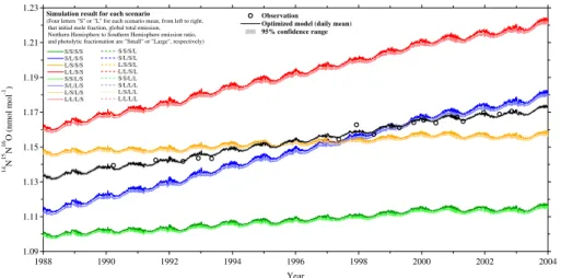
This base emission scenario was multiplied by a single scaling factor that was
ho-mogeneous in space and time, and used for the simulations of each N2O isotopocule.
The model was optimized for both the long-term trends and north-to-south gradients
of tropospheric N2O isotopocules using the observed data. For the long-term trend
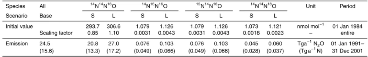
optimization, we prepared small and large emission scenarios for each isotopocule by
10
scaling as mentioned above. The scaling factors and mean annual total emissions for the period 1991–2001 are shown in Table 2, and temporal changes in the emissions are shown in Fig. S1 in the Supplement. To optimize the north-to-south gradients, we
ad-ditionally scaled the emissions using different factors for both hemispheres, but evenly
within each hemisphere. The scaling factors were selected so that the average ratio
15
of Northern Hemispheric emissions (ENH) to Southern Hemispheric emissions (ESH)
for the period 1991–2001 became 0.8 and 1.3 times the ratio of the base emission
scenario for small and largeENH:ESH ratio cases, respectively. By this operation, the
ENH:ESHratio of the base emission scenario of about 1.5 became about 1.2 and 2.0
for the small and large emissions scenarios, respectively. The horizontal and latitudinal
20
distributions of these emissions are shown in Fig. S1. We regard this range (1.2–2.0)
as sufficient, based on our model’s hemispheric transport feature in previous N2O
mod-elling studies, in which the ACTM could well reproduce the north-to-south gradients of
the atmospheric N2O mole fraction with the range of theENH:ESHratio from 1.3 to 1.9
(Ishijima et al., 2010; Thompson et al., 2014b, c). Finally, we prepared four different
25
emission scenarios for each N2O isotopocule: small and large global total emissions,
ACPD
15, 19947–20011, 2015Development of an atmospheric N2O
isotopocule model
K. Ishijima et al.
Title Page
Abstract Introduction
Conclusions References
Tables Figures
◭ ◮
◭ ◮
Back Close
Full Screen / Esc
Printer-friendly Version
Interactive Discussion
Discussion
P
a
per
|
Discussion
P
a
per
|
Discussion
P
a
per
|
Discussion
P
a
per
|
4.1.4 Model run and initial field
We ran the model for the period 1984–2011 starting with well spun-up initial
distribu-tions of atmospheric N2O isotopocule mole fractions. The 3-D initial mole fraction field
was obtained from a spin-up run with a “semi-equilibrium state” for a total of more
than 50 years. “Semi- equilibrium state” here means that the atmospheric N2O trend
5
was mostly maintained at realistic levels, the vertical profile in the stratosphere be-ing also realistic, by balancbe-ing the increasbe-ing surface emissions with the stratospheric
loss. Spin-up is important to simulate atmospheric N2O and to precisely estimate
sur-face emissions of N2O isotopocules by comparing the model and observation data,
because the lifetime of N2O is very long (∼120 years). As for the emissions, the initial
10
mole fraction field was also scaled to prepare small and large initial value cases for the model optimization so that the mole fractions near the surface roughly covered the range of observed mole fractions for each isotopocule (Table 2).
4.2 Model optimization
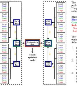
In this study, we optimized the N2O isotopocule model for global total emissions
(us-15
ing the atmospheric long-term trend), the ratio of Northern Hemisphere to Southern Hemisphere emissions (using the atmospheric north–south gradient), and photolytic isotopocule fractionation (using the vertical gradient in the stratosphere) of each
iso-topocule. To accomplish this, we ran the model with several different simulation
sce-narios for each isotopocule, and then, after multiplied by scaling factors, combined the
20
ACPD
15, 19947–20011, 2015Development of an atmospheric N2O
isotopocule model
K. Ishijima et al.
Title Page
Abstract Introduction
Conclusions References
Tables Figures
◭ ◮
◭ ◮
Back Close
Full Screen / Esc
Printer-friendly Version
Interactive Discussion
Discussion
P
a
per
|
Discussion
P
a
per
|
Discussion
P
a
per
|
Discussion
P
a
per
|
4.2.1 Model optimization for tropospheric long-term trend and global total
emissions
To optimize the model, we confirmed that the model system was linear for some points
throughout the atmosphere from the surface to the stratosphere in the N2O simulation,
as follows:
5
S(P3)=f S(P1)+(1−f)S(P2), (10a)
P3=f P1+(1−f)P2. (10b)
Here, P is one of the parameters in the model related to atmospheric N2O
iso-topocule simulation, either the initial value of the atmospheric N2O isotopocule mole
fraction (I), global total emissions (E), the Northern Hemisphere to Southern
Hemi-10
sphere emission ratio (e), or the photolytic fractionation (J). Subscript numbers are
used for the same parameter but the values are different. In Eq. (10a), S(P1), S(P2),
and S(P3) are the results of an atmospheric N2O isotopocule from the simulations,
in which only the parameter P differed among the three simulations and the other
parameters remained the same. f is a scaling factor, generally ranging from 0 to 1.
15
For example, assume that there were two model simulations, in which only the global
N2O emissions are different being 14 and 17 Tg a−1N (E1 and E2), respectively. They
show 300 and 310 nmol mol−1 (S(E1) and S(E2)) at a particular location, date and
time, respectively. If other simulation, in which only the global emission is different
from the above two simulations, shows 303 nmol mol−1 (S(E3)), it is true according
20
to Eqs. (10a) and (10b) thatf =0.7 andE3=f E1+(1−f)E2=14.9 Tg a−1N, because
303=0.7×300+(1−0.7)×310(S(E3)=f×S(E1)+(1−f)×S(E2)). Theoretically, if the
ACPD
15, 19947–20011, 2015Development of an atmospheric N2O
isotopocule model
K. Ishijima et al.
Title Page
Abstract Introduction
Conclusions References
Tables Figures
◭ ◮
◭ ◮
Back Close
Full Screen / Esc
Printer-friendly Version
Interactive Discussion
Discussion
P
a
per
|
Discussion
P
a
per
|
Discussion
P
a
per
|
Discussion
P
a
per
|
S(I1,E3)=fES(I1,E1)+(1−fE)S(I1,E2), (11a)
S(I2,E3)=fES(I2,E1)+(1−fE)S(I2,E2), (11b)
E3=fEE1+(1−fE)E2, (11c)
S(I3,E3)=fIS(I1,E3)+(1−fI)S(I2,E3), (11d)
I3=fII1+(1−fI)I2. (11e)
5
Here,S(I3,E3) is the result of a simulation usingI3andE3, but can actually be produced
by combining four different simulation results:S(I1,E1),S(I1,E2),S(I2,E1), andS(I2,E2),
and the scaling factors fE and fI. Thus, using these four simulation results, we can
determine the optimum values of I and E by assigning optimal values to fE and fI
such that the resultS(I3,E3) best fits the observations (Figs. 2 and 3). More simply, we
10
optimize the “f” values so that combinations of the four model simulation results using
the “f” values fit the observed results in a least square sense. Finally, we can write as
follows:
Observation∼=S(I3,E3) (11f)
Eopt=E3 (11g)
15
Iopt=I3 (11h)
Here,Eopt and Iopt are optimized E and I, respectively. The least square approach is
explained later in this section.
It is known that time series of atmospheric N2O mole fractions and isotopocule ratios
near the surface have almost linear trends over a decadal timescale, so the budget
20
equation for each isotopoculei can be written as follows:
dMi/dt=Ei−kiMi, (12a)
Mi=Mi0+
Z
ACPD
15, 19947–20011, 2015Development of an atmospheric N2O
isotopocule model
K. Ishijima et al.
Title Page
Abstract Introduction
Conclusions References
Tables Figures
◭ ◮
◭ ◮
Back Close
Full Screen / Esc
Printer-friendly Version
Interactive Discussion
Discussion
P
a
per
|
Discussion
P
a
per
|
Discussion
P
a
per
|
Discussion
P
a
per
|
whereMi is the global total mass of an N2O isotopoculei (Tg),Ei is the total emission
(Tg a−1),ki is the mass-weighted global mean chemical loss rate coefficient (a−1), and
Mi0 is the initial mass (Tg). As N2O is fairly well mixed in the troposphere, Mi and
Mi0 can be substituted by FiCi and FiCi0 over a decadal timescale, where Ci is the
atmospheric mole fraction of each N2O isotopoculei (nmol mol−1) at a station and Fi
5
is a conversion factor from mole fraction (nmol mol−1) to mass (Tg), generally around
4.8 Tg per nmol mol−1for14N14N16O (F1), as follows:
dCi/dt=Ei/Fi−kiCi, (13a)
Ci =Ci0+ Z
{Ei/Fi−kiCi}dt. (13b)
In Eq. (13a), the growth rate depends on the surface emission Ei and atmospheric
10
losskiCi. In our simulations, as the loss rate coefficientki is prescribed by the model
meteorology, which is driven by reanalysis data and short- and long-wave radiation
produced by the prescribed fields of greenhouse gases and ozone etc.,Ci itself, as
well asEi, determine the atmospheric trend dCi/dt. Furthermore, Eq. (13b) indicates
thatCi also depends on the initial valueCi0. This means that the model can produce
15
any decadal trend of atmospheric N2O, and certainly the observed trend, if appropriate
values ofCi0andEi are used. However, if the spin-up is insufficient, surface emission
estimated by Eq. (13b) becomes invalid, as mentioned in Sect. 4.1.4. Thus, in this
study we optimized the model for long-term trends of atmospheric N2O isotopocules
to reproduce the results observed at NMY, by using Eqs. (11a)–(11e) and determining
20
optimal values offE and fI. By this process, surface emissions and initial values were
also optimized as shown in Eqs. (11c) and (11e). In the actual optimizations, for all terms in Eqs. (11a)–(11e), the subscript numbers 1, 2, and 3 are substituted by small, large, and optimized, respectively.
A combination of optimal values offE andfI was identified for each isotopocule so
25
that P
i(Cmodeli−Cobservationi) 2
(CXXXi: mole fraction for observation or model at each
ACPD
15, 19947–20011, 2015Development of an atmospheric N2O
isotopocule model
K. Ishijima et al.
Title Page
Abstract Introduction
Conclusions References
Tables Figures
◭ ◮
◭ ◮
Back Close
Full Screen / Esc
Printer-friendly Version
Interactive Discussion
Discussion
P
a
per
|
Discussion
P
a
per
|
Discussion
P
a
per
|
Discussion
P
a
per
|
the initial ranges for searching the optimalf values were set to a relatively wide range
of−1 to 2. The optimalf values were searched by sequentially changing the values, the
intervals and ranges being gradually reduced. In the actual calculation, the first guess
of the combination (fE,1 and fI,1) was obtained with an accuracy of 0.3 in the range
of−1 to 2, the second guess (fE,2 and fI,2) with an accuracy of 0.15 in the ranges of
5
fE,1±0.75 andfI,1±0.75, the third guess (fE,3andfI,3) with an accuracy of 0.075 in the
ranges offE,2±0.375 andfI,2±0.375, and the final results were obtained with an
ac-curacy better than 10−10. All results for thef values eventually became between 0 and
1. The uncertainty caused by the optimization method was estimated using a Monte
Carlo approach for thef values, by assigning random errors to the observational data
10
100 000 times. The random errors were taken from a Gaussian distribution represent-ing the measurement standard error. Uncertainty in the surface emissions was also simultaneously estimated using Eq. (11c). Further details of this optimization proce-dure are provided in the Supplement.
4.2.2 Model optimization for tropospheric north-to-south gradient and the
15
Northern Hemisphere to Southern Hemisphere emission ratio
The Northern Hemisphere to Southern Hemisphere emission ratio (e) was optimized in
almost the same manner as the long-term trend, but more simply (Fig. 2). Time series data, reconstructed from analysis of firn air samples obtained from polar ice sheets (Ta-ble 1; Sect. 3.2) were used for this. As shown in Fig. 2, this optimization was performed
20
after the model had been optimized for the long-term trend, because the emission
ra-tio optimizara-tion has greater freedom with respect to thef values because of the use
of only the interpolar difference (not the absolute value) and the relatively large
mea-surement error compared to the signal. As described in Sect. 4.1.3, we prepared two
different emission scenarios with small and large emission ratios for each isotopocule,
25
ACPD
15, 19947–20011, 2015Development of an atmospheric N2O
isotopocule model
K. Ishijima et al.
Title Page
Abstract Introduction
Conclusions References
Tables Figures
◭ ◮
◭ ◮
Back Close
Full Screen / Esc
Printer-friendly Version
Interactive Discussion
Discussion
P
a
per
|
Discussion
P
a
per
|
Discussion
P
a
per
|
Discussion
P
a
per
|
S(eopt)=feS(eS)+(1−fe)S(eL), (14a)
eopt=feeS+(1−fe)eL, (14b)
whereeS,eL, andeopt are emission scenarios with small, large, and optimized
emis-sion ratios, respectively. As constrained by the observation data, the interhemispheric
differences rather than the raw values of the time series from the firn air analysis were
5
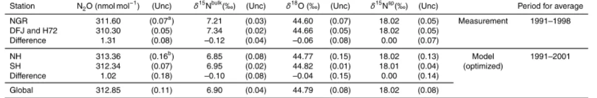
used. The time series was fitted using a spline curve and averaged over the period 1991–1998, and then the value of NGR, after subtracting the mean of the values of DFJ and H72, was used for optimization, because model values in the Southern
Hemi-sphere are already optimized to fit the NMY data, and its standard scales differ from
those for the firn data. The corresponding values are shown in Table 3. More details of
10
this optimization are described in the Supplement.
There is no site preference information (δ15Nα andδ15Nβ, orδ15Nsp) available from
the firn data of Ishijima et al. (2007), and no data on the interhemispheric difference of
site preference have been published to date. To optimize the north–south gradients by
our method, we need to assume a certain value for theδ15Nspgradient. Therefore, we
15
set the value and its uncertainty so that the estimatedδ15Nspvalue and its uncertainty
range for each hemisphere’s total sources did not exceed the range of the δ15Nsp
values for various sources quoted in previous studies (see Fig. 9 in Toyoda et al., 2015).
Following sensitivity tests, we concluded that no interpolar difference of δ15Nsp was
the most reasonable choice (Table 3), which is the same as that assumed in Toyoda
20
et al. (2013). However, as this value is set just for the optimization calculation, we will
not discuss hemisphericδ15Nspvalues any further in this study.
4.2.3 Tuning of photolytic fractionation
Based on some preliminary test simulations, which indicated that the initial photolytic fractionation values given to the model were slightly underestimated, we decided to
25
ACPD
15, 19947–20011, 2015Development of an atmospheric N2O
isotopocule model
K. Ishijima et al.
Title Page
Abstract Introduction
Conclusions References
Tables Figures
◭ ◮
◭ ◮
Back Close
Full Screen / Esc
Printer-friendly Version
Interactive Discussion
Discussion
P
a
per
|
Discussion
P
a
per
|
Discussion
P
a
per
|
Discussion
P
a
per
|
εs derived from Rayleigh plots of observation and model results in the stratosphere.
As described above, the model was first optimized for long-term trends and north– south gradients in the troposphere, but actually the optimizations were completed for
two independent model simulations, in which only photolytic fractionation was different.
Then, the best fit to observed εs were obtained by interpolating the two simulation
5
results.
The εis often used as one of the indices for diagnosing the degree of isotopocule
fractionation caused by photochemical reactions in the stratosphere (e.g., Toyoda et al., 2004; Kaiser et al., 2006). In this study, it was defined as the slope of linear fit-ting to the Rayleigh plot of the isotopocule data, following the definition by Toyoda
10
et al. (2004; referred to as “isotopomer enrichment factors” therein). In the Rayleigh
plot, ln{(δ+1)/(δ0+1)} is plotted against ln{[N2O]/[N2O]0}. Here, δ and [N2O] are
the relative isotopocule ratio difference and N2O mole fraction, respectively, and those
without and with the subscript 0 indicate the values in the stratosphere and of the
ori-gin, respectively. The origin ([N2O]0) is tropospheric N2O, which has not yet suffered
15
from photochemical loss. The air mass in the stratosphere is older than that in the tro-posphere, because it takes time for the tropospheric air to reach the middle to upper part of the stratosphere. The age of the air in the stratosphere is known to range from near zero to more than five years, depending on the altitude, latitude, and season; in the case of the air at the surface this was set to an age of zero years. Therefore, the
20
N2O mole fraction and isotopocule ratios of the origin for the air in the stratosphere
are supposed to be those of the air in the troposphere in the past. In this study, we used the age of air calculated in the model to determine the values for the original air
in the troposphere in the past. The N2O mole fraction and isotopocule ratios observed
at NMY, extrapolated back in time by linear fit, were used as the origin values.
Actu-25
ally, it is difficult to precisely determine the past values, as there are no high-precision
measurement data available before 1990, but we regard the error of around 1 ‰ in the
εs as acceptable for these calculations, considering the large vertical gradients in the
un-ACPD
15, 19947–20011, 2015Development of an atmospheric N2O
isotopocule model
K. Ishijima et al.
Title Page
Abstract Introduction
Conclusions References
Tables Figures
◭ ◮
◭ ◮
Back Close
Full Screen / Esc
Printer-friendly Version
Interactive Discussion
Discussion
P
a
per
|
Discussion
P
a
per
|
Discussion
P
a
per
|
Discussion
P
a
per
|
derestimate the age in the stratosphere. However, even if the age differs by a maximum
of two years between model and observation, theεvalue does not change significantly,
as temporal changes in the N2O mole fraction and isotopocule ratios in the troposphere
are quite small compared with the vertical gradients in the stratosphere.
The underestimation of theεin the model might come from underestimation of the
5
isotopocule fractionation caused by reaction with O(1D) in the model. However, the
absolute value of the experimentally determined fractionation constant for photolysis (von Hessberg et al., 2004) are larger by about one order of magnitude compared to
those for the O(1D) reaction (Kaiser et al., 2002). Overestimation of N2O loss by the
O(1D) reaction may lead to underestimation of the fractionation in the stratosphere
10
by relative increase of the reaction with small isotopic fractionation. Lastly, excessive mixing and transport rates may also cause the apparent stratospheric fractionation to be too small (Kaiser et al., 2006).
We considered that the actual cause for the deficiencies of the stratospheric model
simulations was not so important in this study focusing on the tropospheric N2O, as
15
long as vertical profiles of N2O mole fraction and isotopocule ratios and apparent
isotopic fractionation ε in the stratosphere were realistic. Therefore, we “corrected”
the stratospheric model by artificially enhancing the photolysis isotope fractionation.
To cover the range of observed ε values by model, photolysis rates of 14N15N16O,
15
N14N16O, and 14N14N18O were scaled by a factor of 0.985 (1.5 % reduced
photoly-20
sis for the heavy isotopocules, leading to larger fractionation). This scaling leads to an increase of the fractionation constants by about 14 ‰, outside the uncertainty of the experimental results of von Hessberg et al. (2004; Figs. 3a, b and 4a, b) of about 2 ‰
(1σ) in the stratospherically relevant wavelength range.
Another motivation for adjusting the photolysis rates in the model, as described in
25
Sect. 4.1.1, was that the wavelength resolution of the photolysis calculation in the ACTM was coarse, being only parameterized below 200 nm by a simple scheme, and separated into only three bins above 200 nm, whereas the photolysis of ozone, which is
wave-ACPD
15, 19947–20011, 2015Development of an atmospheric N2O
isotopocule model
K. Ishijima et al.
Title Page
Abstract Introduction
Conclusions References
Tables Figures
◭ ◮
◭ ◮
Back Close
Full Screen / Esc
Printer-friendly Version
Interactive Discussion
Discussion
P
a
per
|
Discussion
P
a
per
|
Discussion
P
a
per
|
Discussion
P
a
per
|
length bins. The coarse wavelength resolution could lead to the uncertainty of N2O
isotopocule fractionations calculated in the ACTM, and the adjustment should take this into account.
The mean ε for all balloon and aircraft observations in the stratosphere (Toyoda
et al., 2004; Kaiser et al., 2006), which is the slope of the linear fit to the Rayleigh
5
plots, was used to tune the photolytic fractionation (Fig. 4). Theεs calculated from two
simulations with the original and 1.5 % reduced photolysis rates, which were already optimized for tropospheric values (Sect. 4.2.1 and 4.2.2), were combined to produce
the observedεs as follows:
εobs≈εtun=fεεorg+(1−fε)εred, (15a)
10
Jtun=fεJorg+(1−fε)Jred=(0.015fε+0.985)Jorg, (15b)
where J is the photolysis rate, and the subscripts tun, org, and red indicate tuned,
simulated using the original photolysis rate (based on von Hessberg et al., 2004), and
1.5 % reduced photolysis rate (Jred=0.985Jorg), respectively. We used the 1.5 %
re-duced photolysis rates only in simulations of14N15N16O,15N14N16O, and14N14N18O,
15
sofε for14N14N16O was always 1. The values offε for the heavier isotopocules were
calculated by assigning the slope values shown in Fig. 4 to Eq. (15a). The results are shown in Table S1. This approach to tuning the photolytic fractionations is an
approx-imation, as Fig. 4 shows that data scatter in the Rayleigh plots and the slopes (εs)
changing with ln{[N2O]/[N2O]0} or altitude, as discussed in Toyoda et al. (2004) and
20
Kaiser et al. (2006). However, we regard this relatively rough tuning approach as suffi
-cient, considering that the main purpose of this study is to reproduce long-term trends
of tropospheric N2O isotopocules and to characterize isotopic signatures of global and
hemispheric total sources. We discuss the impact of the photolytic fractionation on the source estimates later.
ACPD
15, 19947–20011, 2015Development of an atmospheric N2O
isotopocule model
K. Ishijima et al.
Title Page
Abstract Introduction
Conclusions References
Tables Figures
◭ ◮
◭ ◮
Back Close
Full Screen / Esc
Printer-friendly Version
Interactive Discussion
Discussion
P
a
per
|
Discussion
P
a
per
|
Discussion
P
a
per
|
Discussion
P
a
per
|
5 Results and discussion
5.1 Temporal variations at Neumayer station
Figure 5 shows the time series of N2O mole fraction and δ15Nbulk, δ18O, δ15Nα,
δ15Nβ, and δ15Nsp at NMY, Antarctica, derived from both observations (Röckmann
and Levin, 2005) and the optimized model. Standard scales for the observational data
5
are described in Sect. 3.2. The ACTM reproduces the observed results reasonably well overall, showing standard errors of the observational data around the optimize
model data (N2O: 0.1 nmol mol−1,δ15Nbulk: 0.005 ‰, δ18O: 0.005 ‰, δ15Nα: 0.03 ‰,
δ15Nβ: 0.03 ‰, δ15Nsp: 0.05 ‰) comparable to or better than those of the
measure-ments (shown by error bars in Fig. 5). The results indicate that the model optimization
10
was successful. In addition, it is also evident that the agreement between the model and
the observations is much better for mole fraction,δ15Nbulk, and δ18O than forδ15Nα,
δ15Nβ, andδ15Nsp, as the former components are almost overlapping within the error
ranges of the model and observations, whereas the latter components often deviate far from the error ranges. Röckmann and Levin (2005) attributed this data scatter to
ana-15
lytical causes, which makeδ15Nαandδ15Nβ deviate in opposite directions and further
enhancesδ15Nspdeviation from the model results. This is probably a reasonable
expla-nation, considering that the variability ofδ15Nbulk and δ18O are reasonably simulated
by the model despite there being no spatiotemporal variations in the isotopocule ratios of the surface sources given in the model. Meanwhile, Toyoda et al. (2015) showed
20
that δ15Nbulk and δ18O vary in similar directions depending on various source types,
whereasδ15Nspshows a different tendency from them. Certainly, we cannot exclude
the possibility that such features of the site preference data cause more scatter in the atmosphere because of some source-related influence, as Park et al. (2012) raised the
possibility that biomass burning was the cause of increased variability in δ15Nα
dur-25
ACPD
15, 19947–20011, 2015Development of an atmospheric N2O
isotopocule model
K. Ishijima et al.
Title Page
Abstract Introduction
Conclusions References
Tables Figures
◭ ◮
◭ ◮
Back Close
Full Screen / Esc
Printer-friendly Version
Interactive Discussion
Discussion
P
a
per
|
Discussion
P
a
per
|
Discussion
P
a
per
|
Discussion
P
a
per
|
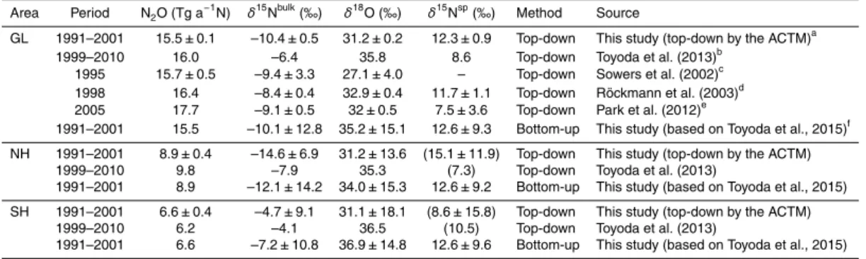
Mole fraction andδ15Nspincrease with time, while the other isotopic components
de-crease. These tendencies are the same as those reported in previous studies, which
found that additional input of N2O from anthropogenic sources with lower δ15Nbulk,
δ18O, δ15Nα, and δ15Nβ, but higher δ15Nsp than those of the tropospheric N2O, is
causing this atmospheric trend; i.e., the so-called Suess effect for N2O isotopocules
5
(Röckmann et al., 2003; Röckmann and Levin, 2005; Park et al., 2012). Toyoda
et al. (2013) showed slightly different trends forδ18O andδ15Nspobserved at Hateruma
station (24◦N, 124◦E; Table 1; Fig. 1), which is strongly affected by nearby sources in
East Asia. Figure 5 also shows long-term change rates for observation and model results. The good agreement is not surprising since the model was optimized to
re-10
produce the observations. In the optimization procedure, only model data for the ob-servation dates were used. For the period 1994–1996, there were five air samples,
which were analysed for N2O andδ15Nbulk (shown by grey color marks in this figure),
but not forδ18O, δ15Nα and δ15Nβ (Röckmann and Levin, 2005). We did not include
such observation data in the optimization, because the procedure always needs all four
15
components (N2O, δ18O, δ15Nα, andδ15Nβ) to handle their mole fractions in the
cal-culation (Sect. 2.2). This actually makes only a small difference in the trend, of about
0.01 nmol mol−1a−1, for the N2O mole fraction, but fortunately, no difference was
evi-dent for the isotopic components.
Seasonal cycle patterns are seen especially clearly in the model. So, here we shortly
20
discuss about seasonality for the atmospheric N2O isotopic components although it
is beyond the scope of the paper. The patterns are more irregular in the observa-tions due to measurement errors and possibly due to some natural causes. For the
observed δ15Nα, δ15Nβ, and δ15Nsp, the large scatter means that it is impossible to
derive statistically meaningful seasonal cycles. The N2O mole fraction is highest in
au-25
tumn to winter, and lowest in spring to summer, the opposite is observed forδ15Nbulk
and δ18O, both in the observations and the model. Furthermore, their seasonal