www.the-cryosphere.net/7/1679/2013/ doi:10.5194/tc-7-1679-2013
© Author(s) 2013. CC Attribution 3.0 License.
The Cryosphere
Changing basal conditions during the speed-up of Jakobshavn
Isbræ, Greenland
M. Habermann1, M. Truffer1, and D. Maxwell2
1Geophysical Institute, University of Alaska Fairbanks, Fairbanks, AK 99775-7320, USA
2Department of Mathematics and Statistics, University of Alaska Fairbanks, Fairbanks, AK 99775, USA
Correspondence to:M. Habermann ([email protected]) Received: 30 April 2013 – Published in The Cryosphere Discuss.: 1 June 2013
Revised: 26 September 2013 – Accepted: 9 October 2013 – Published: 7 November 2013
Abstract. Ice-sheet outlet glaciers can undergo dynamic changes such as the rapid speed-up of Jakobshavn Isbræ fol-lowing the disintegration of its floating ice tongue. These changes are associated with stress changes on the bound-ary of the ice mass. We invert for basal conditions from sur-face velocity data throughout a well-observed period of rapid change and evaluate parameterizations currently used in ice-sheet models. A Tikhonov inverse method with a shallow-shelf approximation forward model is used for diagnostic inversions for the years 1985, 2000, 2005, 2006 and 2008. Our ice-softness, model norm, and regularization parameter choices are justified using the data-model misfit metric and theLcurve method. The sensitivity of the inversion results to these parameter choices is explored. We find a lowering of effective basal yield stress in the first 7 km upstream from the 2008 grounding line and no significant changes higher upstream. The temporal evolution in the fast flow area is in broad agreement with a Mohr–Coulomb parameterization of basal shear stress, but with a till friction angle much lower than has been measured for till samples. The lowering of ef-fective basal yield stress is significant within the uncertain-ties of the inversion, but it cannot be ruled out that there are other significant contributors to the acceleration of the glacier.
1 Introduction
Ice-sheet outlet glaciers can evolve much more dynamically than formerly thought (Truffer and Fahnestock, 2007). Mod-eling and understanding the processes involved in these rapid changes is challenging. Despite the abundant surface data
available from satellites, conditions within the ice and at the base of the ice are still difficult to observe, but these are cru-cial components of successful prognostic ice-sheet models.
Jakobshavn Isbræ is one of the most active outlet glaciers in Greenland and has a century-long record of observations (Weidick et al., 1990). This outlet glacier drains about 5.5 % of the ice-sheet area (Rignot and Kanagaratnam, 2006) and has undergone a rapid evolution in the last two decades. Dur-ing the 1990s Jakobshavn Isbræ had a relatively stationary terminus position (Sohn et al., 1998), but starting in 1997, increased thinning of the floating ice tongue was observed (Thomas et al., 2003), followed by the retreat and complete disintegration of the 15 km-long ice tongue in 2003 (Podlech and Weidick, 2004). Coinciding with the retreat of the ice front, the ice underwent a significant speed-up, almost dou-bling its speed by 2003 (Joughin et al., 2004). After the disin-tegration of the ice tongue, the ice front retreat and the accel-erations in speed have decreased but are still ongoing today (Joughin et al., 2012).
leads to an increase in sliding speed (Meier and Post, 1987; Pfeffer, 2007). The third process is a steepening of slopes induced by the strong thinning on the main trunk, causing the speed-up to diffuse inland (Joughin et al., 2008b; Payne et al., 2004). Other possible processes include weakening of the ice in the lateral shear margins and increase in basal wa-ter pressure through changes in the hydrological system (Van Der Veen et al., 2011). The observational evidence strongly favors an acceleration mechanism that is ocean and terminus driven (Motyka et al., 2011; Joughin et al., 2012).
The well-observed changes of Jakobshavn Isbræ make it possible to investigate temporal changes in effective basal yield stress by inverting surface velocities for different years. (Joughin et al., 2012) performed one inversion for the 1990s velocities and one for the 2009 velocities. Here we expand on this by inverting all available velocity fields and by conduct-ing an extensive parameter study to discuss the robustness of the inversion results.
To take advantage of the wealth of surface data, we use inverse methods to reconstruct conditions at the ice-bed boundary. Inverse methods were first introduced to the field of glaciology by (MacAyeal, 1992), and have since been used, improved and extended in multiple studies (e.g., Truffer, 2004; Maxwell et al., 2008; Raymond and Gud-mundsson, 2009). Much like other recent studies (Morlighem et al., 2010; Konovalov, 2012; Petra et al., 2012), we use a Tikhonov regularization to stabilize the solution, and we focus on justifying the choices that accompany this method.
In this study we investigate different parameter choices for the effective basal yield stress inversion of Jakobshavn Isbræ, where decisions are mostly based on the data-model misfit metric. The chosen parameters are then used to invert, for effective basal yield stress, the surface velocity data sets of the years 1985, 2000, 2005, 2006 and 2008. We discuss the robustness of these results and the agreement with commonly used parameterizations of effective basal yield stress.
2 Methods
2.1 Model
To investigate spatial changes and characteristics of basal shear stress, we use the shallow-shelf approximation (SSA) (Morland, 1987) as the forward model in a Tikhonov inver-sion.
2.1.1 Forward model
The Parallel Ice Sheet Model (PISM) is a 3-D thermome-chanically coupled hybrid ice-sheet model that solves a com-bination of the shallow-ice and shallow-shelf approximations (Bueler and Brown, 2009, http://www.pism-docs.org). In this study only the SSA is used and the vertically averaged ice softness does not vary horizontally. Details about the SSA
can be found in Schoof and Hindmarsh (2010) and the imple-mentation in PISM is described in Bueler and Brown (2009). We follow Joughin et al. (2012) and use the SSA as a for-ward model. Despite being depth-averaged the model does consider membrane stresses, vertical shear on the other hand is not considered. Ignoring vertical shear can be justified by the weak temperate basal ice layer that is present at Jakob-shavn Isbræ, which concentrates vertical motion near the bot-tom, and by the weak bed compared to the driving stresses, which leads to motion that is dominated by basal ice motion, at least in the lower regions of the glacier (Lüthi et al., 2002). However, it is important to keep in mind that the results de-rived in this paper are effective basal yield stress fields that are consistent with the SSA and surface observations, and might not reflect actual physical till properties.
The basal shear stressτbis parametrized through a power law:
τb=τc |u|q−1
uqthreshold
u, (1)
whereuis the basal sliding velocity, and the threshold ve-locityuthresholdis set to 100 m a−1. The purely plastic case is achieved by settingq=0, whereasq=1 leads to the com-mon treatment of basal till as a linearly viscous material: τb,x=γ uand τb,y=γ v, where γ≥0 is a scalar function of position, called the basal stickiness. When settingq=1 the basal stickiness,γ, and the effective basal yield stress, τc, are related throughγ = τc
uthreshold. Here, instead of setting q=1 and solving forγ we solve forτc, which has units of stress and is the basal yield stress ifq=0. We approximate the perfectly plastic case by settingq=0.25 for this study and callτctheeffective basal yield stress. This is the stress that occurs at the base when it is sliding atuthreshold. Ifq is close to zero, and if there is reasonable sliding at the base, we can expect that the stress at the base will be close toτc. As such it plays the role of a yield stress. Test inversions with q=0.1 and q=0.001 for the 1985 and 2006 data sets re-sult in differentτc values, but the pattern and amplitude of changes inτcremain and the main conclusions of this paper are unchanged. The positivity ofτcis enforced by solving for ζ inτc=τc,scaleexp(ζ )whereτc,scaleis a scale parameter to keepζ of order 1 for typical values ofτc.
The chosen values for q and uthreshold used here were found to provide the best representation of observed ice mo-tion (Bueler, personal communicamo-tion, 2012). As menmo-tioned before, the results derived in this paper are effective basal yield stress fields that are consistent with our model choices and surface observations, and might not reflect actual physi-cal till properties. The main conclusions of this paper, namely a weakening of the till near the terminus, remain valid for dif-ferent choices ofqanduthreshold.
We assume the instantaneous (diagnostic) surface veloc-ities represent instantaneous deformation rates and effec-tive basal yield stress at depth. In other words, no time-dependent (prognostic) runs are performed and instead the forward model calculates a velocity field from effective basal yield stressτc, and the inversion is an attempt to recoverτc from measured surface velocities at a given time.
2.1.2 Inferring effective basal yield stress
Solving for the effective basal yield stress distribution is an ill-posed inverse problem, one consequence being the mul-titude of possible solutions. Often these ill-posed problems can be stabilized by imposing additional constraints that bias the solution. This is referred to as regularization (Aster et al., 2005). We apply the widely used Tikhonov regularization, which defines a cost functional,I (τc, α), with an added
reg-ularization term:
I (τc, α)=α M2+N2, (2)
M2= 1 ||
Z
ku(τc)−uobsk2d (3)
N2= 1 ||
Z
cL2(τc−τ prior
c )2+K2cH1|∇(τc−τ prior c )|2d,
(4) whereMis the data-model misfit,Nis the model norm (reg-ularization term) andαis the regularization parameter. Note that, depending on the application,αis sometimes attached to the model norm instead of the data-model misfit. This only changes the value ofα, but not any of the results.
We discretize the functional I (τc, α) by representing τc via a finite-element approximation, and by computing a fi-nite element solution foru(τc). Doing so determines a dis-cretized functional Idisc:Rn→R, where n is the number of grid points whereτc is defined. The gradient of this dis-cretized functional (with respect to the standard inner prod-uct onRn) can be computed exactly; the gradient of the term M2is determined by a discrete computation similar to the continuous computation of theL2gradient described in the Appendix of (Habermann et al., 2012), whereas the gradient ofN2(which is quadratic inτc) is computed trivially. A min-imum of the discrete functional can then be sought by any one of a number of gradient-based minimization algorithms. We use a limited-memory, variable-metric method from the Toolkit for Advanced Optimization (TAO) (Munson et al., 2012) to seek an exact minimum of the discretized cost func-tion,I (τc, α).
Assuming that there is a unique minimum (which is true at the very least whenαis small), an exactly computed min-imum of the discretized functional will be independent of the numerical method used to find it. The areais defined by grounded ice (determined by hydrostatic equilibrium) and the consistent availability of velocity observations over the time periods considered. This is only part of the model do-main (see Fig. 1), but all interpretations will be restricted by it. Below we refer toas the ‘misfit area’. The model norm in Eq. (4) is composed of two parts: the EuclidianL2norm and a SobolovH1norm that measures the function’s rough-ness. The factorscL2 andcH1 determine the relative weights of these two norms. The variableKdefines a typical length scale to rescale theH1norm (set to 5×10⁴m). The model norm is measured as a difference from a prior estimateτcprior. A choice ofcL2=1 andcH1 =0 results in a pureL2model norm, which gives preference to solutions with a small de-parture from the prior estimate. At the other end of the spec-trum, settingcL2=0 andcH1 =1 results in a pureH1model norm, which biases the solution towards smooth differences to the prior estimate.
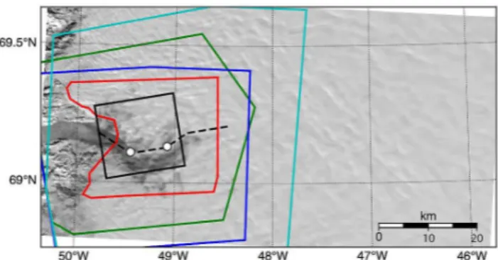
Fig. 1. Model domain (entire area shown) with MODIS image for reference (single pass MODIS image, spring 2001, courtesy of M. Fahnestock). Also shown are the extent of the higher resolu-tion bed topography (cyan), 2007 DEM (green), 1985 DEM (blue), misfit area (red), straightened centerline (dashed black), the white circles mark the two “bends” that are mentioned later on and the area later shown in all the map-view figures (solid black).
parameterα determines a unique value for the data-model misfit and hence the model norm. To discuss the choice of regularization parameter,α, we introduce the following vo-cabulary. The observation error is defined asTobs, the sys-tem error is defined asTtot=Tmod+Tobs, where the mod-eling error,Tmod, contains errors from model simplifications and errors in input parameters such as ice geometry. For an ill-posed inverse problem it is not desirable to find an exact minimizer of the data-model misfit,M, because this would lead to overfitting of the data (Habermann et al., 2012). The achieved data-model misfit should not be smaller than the combined error of observations, model simplifications, and parameter choices,Ttot. On the other hand, if the data-model misfit is too large, because we are forcing a high degree of smoothness in the effective basal yield stress solution, the highest possible resolution is not achieved and the data are underfit.
There are different ways to choose the regularization pa-rameterα. The “discrepancy principle”, which sets the data-model misfit equal toTtot is useful in situations where all errors in the system are known or where the observation er-rors can be estimated and the model erer-rors are negligible. For the Tikhonov regularization the discrepancy principle cannot be applied directly. Instead a value for the regularization pa-rameterαis chosen and the resulting data-model misfit value is compared toTtot, if it is known.
A more common situation arises when the errors in the system are not known. It is particularly difficult to quantify model errors that originate from the use of lower order for-ward models, such as the SSA, and the effect of poorly con-strained model parameters, such as the ice softness and bed topography, that are not part of the inversion procedure. In such cases it is possible to use a heuristic “Lcurve” method (Jay-Allemand et al., 2011; Gillet-Chaulet et al., 2012). It has been proposed for its ease of use, despite some
poten-tial shortcomings (discussed in e.g., Vogel, 1987, ch. 7). In theLcurve method the data-model misfit is plotted against the model norm (either on a log–log or a linear scale). This curve typically has anLshape and the regularization param-eter value corresponding to the “corner” of the curve, which is usually defined as the point of highest curvature, is chosen. The rationale behind this choice of regularization parameter is that past this corner even a small improvement in the data-model misfit can only be achieved through a large increase in the roughness of the solution.
The actual value of the data-model misfit depends on the misfit area. Therefore, the data-model misfit value can only be used to compare different inversion results if the misfit areas are identical. Here we use the same misfit area for all years, given by the consistent availability of velocity obser-vations and by grounded ice (the 2008 grounding line lim-its the misfit area in the terminus region). This misfit area is shown in Fig. 1. An appropriate data-model misfit can still lead to overfitting in some subareas and underfitting in oth-ers.
2.2 Data
A combination of previously published airborne and space-borne data sets, collected between 1985 and 2008, are used as input to the model. All data sets are given on or interpo-lated to a 500 m×500 m grid, which is the grid size chosen for the model. Table 1 gives a summary of surface elevations and velocity fields used for each year.
2.2.1 Surface elevation
We used the 1985 and 2007 digital elevation models (DEM) derived by Motyka et al. (2010). The 1985 DEM is based on aerial photos, whereas the 2007 DEM was derived from SPOT-5 imagery under the SPIRIT (stereoscopic survey of Polar Ice: Reference Images and Topographies) Polar Dali Program (Korona et al., 2009). To extend the model domain, we took lower resolution surface elevations given by Bam-ber et al. (2001), and substituted the high resolution DEMs in the coverage area. As a result there are sharp transitions from the high resolution DEM to the low resolution DEM. These sharp transitions result in unphysical driving stresses and we smooth the DEM by performing a short (2 week) non-sliding shallow-ice approximation run on a regional scale with PISM. The model domain was chosen beyond the ex-tent of the high resolution DEMs to minimize the impact of boundary effects on the results. Model results are only eval-uated within the coverage area of the high resolution DEMs (Fig. 1).
Table 1.Summary of velocity fields and surface elevation data sets used for each year, including details on acquisition dates and source references. The 2007 SPOT DEM that is mentioned was obtained 24 July 2007. The outline of the glacier is given by the ice thickness of the DEM for each inverted year. The misfit area is the same for all years (see Fig. 1).
Year Period covered by vel. field Reference for vel. Date of surface DEM Reference for DEM
1985 7–24 July 1985 courtesy of M. Fahnestock 24 July 1985 (aerial photo) (Motyka et al., 2010) 2000 3 September 2000–24 January 2001 (Joughin et al., 2010) 2007 SPOT DEM – dh/dtfor (Motyka et al., 2010),
(RADARSAT-1 satellite) 2000 courtesy of B. Smith (Joughin et al., 2012) 2005 13 December 2005–20 April 2006 (Joughin et al., 2010) 2007 SPOT DEM – dh/dtfor (Motyka et al., 2010), (RADARSAT-1 satellite) 2005 courtesy of B. Smith (Joughin et al., 2012) 2006 Winter average 2006–2007, (Joughin et al., 2010) 2007 SPOT DEM – dh/dtfor (Motyka et al., 2010), no further detail given 2006 courtesy of B. Smith (Joughin et al., 2012) 2008 Winter average 2008–2009, (Joughin et al., 2010) 2007 SPOT DEM – dh/dtfor (Motyka et al., 2010), no further detail given 2008 courtesy of B. Smith (Joughin et al., 2012)
2.2.2 Bed elevation
The bed DEM was developed at the University of Kansas using data collected by their airborne depth-sounding radar (Plummer et al., 2008). It is important to point out that the bed elevation is one of the model input fields with significant uncertainties. Even though the Jakobshavn Isbræ drainage area has been flown repeatedly with a radar depth sounder, the deep trough with its steep margins often does not allow for clear bed returns.
We investigate the influence of bed topography on the in-version results in (Habermann, 2013) and we find that errors in bed topography lead to residuals that are larger than the residuals due to errors in velocity observations. This large ex-pected error is consistent over all inversions performed here and we do not expect a significant influence on the changes in effective basal yield stress.
2.2.3 Ice flow velocity
NASA’s Making Earth System Data Records for Use in Re-search Environments (MEaSUREs) program, provides an-nual ice-sheet-wide velocity maps for Greenland, derived us-ing Interferometric Synthetic Aperture Radar (InSAR) data from the RADARSAT-1 satellite. The data set contains ice velocity data for the winter of 2000–2001 and 2005–2006, 2006–2007, and 2007–2008 acquired from RADARSAT-1 InSAR data from the Alaska Satellite Facility (ASF), and a 2008–2009 mosaic derived from the Advanced Land Ob-servation Satellite (ALOS) and TerraSAR-X data (Joughin et al., 2010). Here we are using all available velocity data sets except for 2007–2008, which contains data gaps.
For the 1985 inversion we use a velocity data set derived from feature tracking of orthophotos used in the formation of the 1985 DEM (Motyka et al., 2011).
2.2.4 Model domain
The forward model has to be evaluated repeatedly in the in-version, but all runs are instantaneous. This eliminates the
need for a careful treatment of the boundary areas or the solu-tion of the SSA in the entire drainage area, as done in regional time-dependent models. Instead we choose a limited model domain for efficiency, but include enough area around the used data sets (DEMs and bed elevation) to minimize bound-ary effects. We evaluate results spatially and along a cen-terline, which was extracted by approximately following the minimum bed elevation (Fig. 1). Figure 1 shows the model domain and the areas of high resolution DEMs and bed el-evation as well as the misfit area used to calculate the data-model misfit in the inversion. The SSA is solved over the entire model domain, but only velocity data within the misfit area is used to adjust the effective basal yield stress. Results are only interpreted within the misfit area, which is taken to be the same for all years. Areas outside the misfit area are shaded or excluded in all figures.
3 Choices in forward model and inversion
The model outlined above contains several poorly con-strained parameter choices. In this section we discuss the choice for ice softnessAin the forward model, the choice of model norm in the regularization term, the prior estimate for the effective basal yield stress, and the magnitude of the regularization parameter. For the model norm and the prior estimate of effective basal yield stress we used the 2006 data set, for all other parameters all inverted years where consid-ered to determine the value. Final parameter choices were made after several iterations. We arrived at the following de-faults values:
– Ice softness:A=2.5×10⁻²⁴Pa−3s−1
– Model norm:cL2=0,cH1=1
– Prior estimate:τcprior=1.4×10⁵Pa
Below we will discuss each choice by studying the effects of varying one parameter at a time, while holding the others at their default value.
3.1 Ice softness
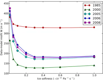
The forward model contains many parameter choices, here we only discuss the ice-softness parameter. All other values for the forward model are discussed in Sect. 2.1.1. Default values, or values that have proven to be good choices in other studies are used whenever possible. The SSA uses a viscos-ity that is dependent on a vertically averaged ice-softness parameterA which in turn depends on the temperature of the ice. Temperature has only been measured in a few bore-holes (Lüthi et al., 2002) and its spatial distribution is not known. Here the vertically averaged ice softness does not vary horizontally for the entire model domain and we test different ice-softness values. A spatially variable ice softness would lead to effective basal yield stress fields that are con-sistent with the ice softness and therefore different than the effective basal yield stress fields found here. Nonetheless, we would expect all main findings about the changes and sensitivities of effective basal yield stress to stay true. Ad-ditionally, we conducted time-dependent numerical experi-ments (spin-ups), where not only the ice flow but also tem-perature fields were computed. These experiments show little horizontal variability in the vertically averaged ice softness.
Suggested values of ice softness in Cuffey and Paterson (2010, chapter 3.4.6, p. 72 ff) range from 0.01×10⁻²⁴Pa−3s−1 for ice at −40◦C to 2.4×10⁻²⁴Pa−3s−1 for temperate ice, while values as high as 9.3×10⁻²⁴Pa−3s−1 have been reported from laboratory tests (Budd and Jacka, 1989). Higher values of ice softness are often used and justified by the anisotropy of ice or effects of grain size and/or impurities (Lüthi et al., 2002).
The achieved data-model misfit for different ice soft-ness (Fig. 2) shows that only very hard ice (low A) leads to a marked increase in the data-model misfit. This con-firms the finding of Joughin et al. (2012) that a hard ice model is not a good representation of the ice rheology of Jakobshavn Isbræ. On the other hand, Joughin et al. (2012) find with a terminus-driven model that a soft-ice model (A=10×10−24Pa−3s−1) does not transfer seasonal changes far enough inland. Here the ice-softness value 2.5× 10⁻²⁴Pa−3s−1 is chosen for all years as a compromise be-tween 2 and 3×10⁻²⁴Pa−3s−1, which give the lowest data-model misfit for 1985, 2000 and 2005, 2006, 2008. This ice softness is equivalent to an isothermal ice column with a tem-perature of∼ −3◦C using the flow law temperature depen-dence given by (Cuffey and Paterson, 2010). For compari-son, at a site on the ice sheet adjacent to the ice stream (Lüthi et al., 2002) measured borehole temperatures that provide an estimate of ice softness equivalent to∼ −15◦C isothermal
0.2 0.4 0.6 0.8 1.0 Ice softness (×10−23 Pa−3 s−1)
100 150 200 250 300 350 400 450
Da
ta-mo
de
l m
isfi
t
M
(m
a
−
1)
1985
2000
2005
2006
2008
Fig. 2.Data-model misfitM(Eq. 3) for different ice-softness val-ues for all years. Hard ice (small value of ice softnessA) leads to a marked increase in data-model misfit, whereas softer ice only slightly increases the data-model misfit. We choose the ice soft-nessA= 2.5×10⁻²⁴Pa−3s−1 for all years and the range from 2–3×10⁻²⁴Pa−3s−1is discussed.
ice, indicating our chosen ice softness has some enhancement relative to the borehole.
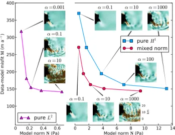
3.2 Model norm
The regularization term of the cost function contains a model norm (Eq. 4). This term is necessary to stabilize the inver-sion. Choosing a model norm biases the solution and needs to be considered in the interpretation. As outlined in the Meth-ods Sect. 2.1.2, the type of model norm used here allows for a bias towards (1) “small” solutions, where the departure from a prior estimate of effective basal yield stress is penal-ized, (2) “smooth” solutions where the derivative ofτc−τcprior is held small, which tends to preserve the shape ofτcprior, or (3) a mix between these two options.
0 0.2 0.4 0.6 Model norm N (Pa) 100
150 200 250 300 350 400
Da
ta-mo
de
l m
isf
it
M
(m
a
−
1)
pure
L20 2 4 6 8 10 12 14 Model norm N (Pa)
pure
H1mixed norm
α =0.1 α =10
α =100 α =1000
α =0.1 α =10
0 10 20
km
α =1000 α =0.001
α =0.1
α =10
Fig. 3.Lcurves for three different model norms; pureH1(cL2=0,
cH1=1), pureL2(cL2=1,cH1=0) and a mixed norm (cL2= 0.9,cH1=0.1). All inversions are for the 2006 velocity data with ice softnessA=2.5×10⁻²⁴Pa−3s−1. The small insets show map views ofτcsolutions for different regularization parameters to
il-lustrate the increase in small-scale features with higherα’s.
but with similar limits for data-model misfits. This can be an indication of the total error,Ttot, in the system.
The pureL2norm produces large jumps in effective basal yield stress, especially with higher regularization parameter values, making it more sensitive to the choice ofα. Here we prefer the pureH1norm solution because the non-localized nature of the SSA does not account for small-scale features in effective basal yield stress. Additionally, as long as the reg-ularization parameter is chosen to yield similar data-model misfit values, the choice of norm influences the solution only within an acceptable range (see Sect. 5.1).
3.3 Prior estimate
In Tikhonov regularization, the cost function (Eq. 2) is min-imized, and a prior estimate of effective basal yield stress is necessary as a starting point for the iterations and for the model norm term. Within the misfit area the latter seems to outweigh the former. A prior estimate commonly used in glaciology is the driving stress field divided by two (Joughin et al., 2004). This choice was suggested because in the shallow-ice approximation the driving stress is locally bal-anced by the basal shear stress, but this is not necessarily the case for the SSA, where membrane stresses are considered.
Figure 4 shows two Tikhonov inversions with the prior es-timate set toτd/2 and to a constant value. Both of the re-sulting effective basal yield stress fields lead to almost iden-tical residual velocity fields; in other words both solutions can account for the main features of the observed velocities. Small-scale features that are introduced in theτd/2 prior es-timate remain unchanged because they do not affect the
ve-Fig. 4.Influence of different prior estimates. Inversions with 2006 velocity data and a prior estimate of effective basal yield stress of (Top) τcprior=τd/2 and (Bottom) τcprior=1.4×10⁵Pa. The
columns show the prior estimate, the inferred effective basal yield stress, the change of the prior to the modeledτcand the residual in
velocity (|uobs−umod|). PureL2model norm,α=0.1.
locity field sufficiently. The commonly used L2 norm was applied for this figure; theH1 norm would exacerbate the problem because the shape of the initial estimate tends to be preserved.
Without prior knowledge about the basal shear stress a constant prior estimate is most appropriate to avoid intro-ducing small-scale features that may not be real. For the pureH1 model norm adding a constant value toτcprior will not influence the solution inside the misfit area. But we find that the inversion converges only for values within a certain range (approximately 5×10⁴–8×10⁵Pa). Therefore a good prior estimate could be the average of τd inside the misfit area (here:τd≈1×10⁵Pa). Here we performed an inversion and used the value of modeled effective basal yield stress along the centerline at the upstream edge of the misfit area as the prior estimate (1.4×10⁵Pa). In this way the algorithm does not have to introduce extreme basal shear stress values to compensate for values outside the misfit area that lead to wrong ice velocities. All prior estimates in the remainder of this study were set to 1.4×10⁵Pa.
3.4 Regularization parameter
0 2 4 6 8 10 12 14 Model norm N (Pa)
100 150 200 250 300 350 400 450
Da
ta-mo
de
l m
isfi
t
M
(m
a
−
1)
α
0.1
1
10
100
1000
Year1985
2000
2005
2006
2008
Fig. 5.Lcurves for all years plotted on a linear scale. The range of regularization parameters isα=0.1 - 1×10³. Based on this figure α=10 is chosen for all years.
Data-model misfit values in Fig. 5 do not reach below 100 ma−1, which is much higher than the expected root mean square error in surface velocity observations: assuming a 3 % error (Joughin et al., 2012) the root mean square error over the misfit area is∼7 m a−1. Errors are thus dominated by those introduced by the simplified model and/or geometry input fields. The high data-model misfit ensures that no fitting of the observed surface velocity data occurs, but over-fitting due to the model and parameter errors would still be a possibility without the regularization term. SinceTobs is much smaller than the data-model misfit, we use theLcurve method to improve parameters of the model such as the ice softness.
4 Results
Inversions for all years with the parameter choices discussed above are shown in Fig. 6. All inversions reproduce the over-all pattern of observed surface velocities. This shows that, in general, our data and model choices are capable of reproduc-ing the observations by only adjustreproduc-ing effective basal yield stress. But a small data-model misfit by itself does not speak to the quality of the resulting effective basal yield stress so-lution.
The first leg (lower 5 km of the glacier) shows a trend from higher to lower effective basal yield stresses over the years. Additionally, a slight widening of the area with low effec-tive basal yield stresses is evident. The 2008 inversion results show continued widening, but the low effective basal yield stress area does not extend as far inland as in the 2006 re-sults. Despite the use of independently produced DEMs and observed surface velocity data sets, the general spatial dis-tribution of effective basal yield stress outside of the main
Fig. 6. Inversion results for 1985, 2000, 2005, 2006 and 2008. The columns show the modeledτc(logarithmic scale), the velocity
residual (|uobs−umod|), the relative velocity residual (100|uobs− umod|/uobs), the observed velocitiesuobsand the modeled
veloci-tiesumod. The area past the 2008 grounding line is not included in
the misfit area and is blacked out.
τc
1985
104 105
Pa
2000
2005
2006
0 10 20
km
2008
Fig. 7.Close-up of inversion results for 1985, 2000, 2005, 2006 and 2008. The columns show the modeledτc for each year. The
area past the 2008 grounding line is not included in the misfit area and is blacked out.
fast flowing glacier remains fairly constant in all inversions compared to the large changes in the first leg. This consis-tency across years in areas with minimal observed changes in geometry and flow is encouraging and justifies the use of constant parameters for all inversion runs.
Our main area of interest is the lower glacier with the largest changes in effective basal yield stress across the years. This area entails high values of observed surface velocities and a deep trough in the bed topography. Residual velocities (difference of modeled and observed) are generally high in this area of fast flow, but relative residuals are in fact similar or lower than in the slow flowing areas (Fig. 6).
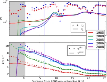
105 106
Pa
τd
τb
0 5 10 15 20 25
Distance from 2008 grounding line (km) 2
4 6 8 10
km
a
−
1
1985
2000
2005
2006
2008
uobs
umod
Fig. 8.Inferred basal shear stress,τb, along centerline for all years.
Area outside of misfit area is shaded gray and the blue vertical lines show the position of the two bends in the centerline. (Top) Crosses mark the driving stresses,τd, for the years 1985 and 2006. The sharp
peak inτboccurs at the grounding line for each year. (Bottom)
Mod-eled (solid lines) and observed (points) velocities for all years.
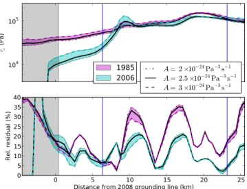
seen in the spatial distribution of effective basal yield stress, the values in the first leg are clearly lowered compared to higher upstream, and they generally decrease over time. De-spite minimal changes in driving stress from 1985 to 2006, the basal shear stress changes significantly over this time pe-riod. In 2000 only a lowering close to the first bend is visi-ble, whereas basal shear stress close to the terminus increases compared to 1985. Past the first bend, the inverted basal shear stresses are generally higher; for 2008 the average value of τbin the first leg is 0.2×10⁵Pa, whereas the average value between the first and the second bend is 1.8×10⁵Pa. Up-stream of the first leg no clear trend in basal shear stress is visible, which is in contrast to the general increase in basal shear stress in this area inferred by Joughin et al. (2012). The basal shear stress accounts for about 20–40 % of the driving stresses along the entire centerline, with a few single peaks reaching 80–100 % of the driving stresses.
5 Discussion
5.1 Robustness of inversion
The solution to our inverse problem is not unique, many of the parameters are not well constrained and a range of pa-rameter choices would be equally acceptable. The emphasis here is on temporal changes in effective basal yield stress, and little significance should be given to the actual value of the stress in a given inversion. To evaluate the robustness of our results, we explore a range of parameters for the years 1985 and 2006.
We chose an ice-softness value of 2.5×10⁻²⁴Pa−3s−1 for all years, while the minimum data-model misfit val-ues are reached for ice-softness valval-ues between 2 and 3× 10⁻²⁴Pa−3s−1 (see Fig. 2). Figure 9 shows an envelope of solutions of effective basal yield stress along the center-line for this range of ice softness. The solutions for A= 3×10⁻²⁴Pa−3s−1lead to generally higherτcvalues than the A=2×10⁻²⁴Pa−3s−1solutions, because softer ice leads to a more localized stress balance and therefore to higher values in effective basal yield stress. The 2006 effective basal yield stress solution exhibits a higher sensitivity to changes in ice softness and the effective basal yield stress is affected most just upstream of the first bend. It is important to keep in mind that we are using a constant value of ice softness over the en-tire model domain. Larger variations of effective basal yield stress are possible for more realistic representations of the temperature distribution in the ice. As a thermomechanically coupled ice-sheet model, PISM is capable of producing real-istic ice temperature fields, which could be achieved through spin-ups. But it is not clear which effective basal yield stress values to use for such a spin-up. Joughin et al. (2009) for ex-ample used iterative spin-ups to find an ice temperature field that is consistent with the effective basal yield stress.
One of the most important sources of uncertainty is the choice of regularization parameter. As mentioned before, it is not straight forward to choose the exact location of the “corner” in theL curve. In other studies the regularization parameter is chosen by calculating the point of maximum curvature (Vogel, 1987, ch. 7.4). But even when this point is calculated exactly, theLcurve criterion remains an approxi-mate method. Therefore, we chose the approxiapproxi-mate value of α=10 and an upper and lower bound (α=3 andα=30). Figure 10 shows that the choice of regularization parame-ter mostly affects the first leg where a smaller data-model misfit in velocities is expensive (in the model norm sense) because the narrow trough makes abrupt changes inτc nec-essary. The data-model misfit is a root mean square over the misfit area, meaning that local under- or overfitting is possi-ble (and very probapossi-ble). When plotting the data-model misfit relative touobsalong the centerline for different regulariza-tion parameters (Fig. 10), it becomes clear that in the first leg the fit to velocity observations is still improving, unlike in areas higher upstream. A higherαcould be justified when focusing on the inversion results ofτcin the first leg.
104
105
τc
(Pa
)
1985
2006
A = 2 ×10A = 2.5 ×10⁻²⁴−24PaPa−3−3s−1s−1A = 3 ×10⁻²⁴Pa−3s−1
0 5 10 15 20 25
Distance from 2008 grounding line (km) 0
5 10 15 20 25 30 35 40
Rel. residual (%)
Fig. 9.Robustness of effective basal yield stress results for a range of ice-softness values (same centerline as Fig. 8). (Top) Softness values of 2×10⁻²⁴Pa−3s−1and 3×10⁻²⁴Pa−3s−1are shown as lower and upper envelopes, respectively, the black line indicates the 2.5×10⁻²⁴Pa−3s−1solution for both years. (Bottom) Data-model misfit of velocities relative to observed speed for the range of ice softness.
104
105
τc
(Pa
)
1985
2006
α = 3α = 10α = 30
0 5 10 15 20 25
Distance from 2008 grounding line (km) 05
10 15 20 25 30 35 40
Rel. residual (%)
Fig. 10.Robustness of effective basal yield stress for regularization parameter values,α=3 (upper envelope) andα=30 (lower enve-lope), the black line indicates theα=10 solution.
for this regularization parameter is shown as well in Fig. 11. The value of the modeledτc is generally lower in this case and displays sharper features, while the improvement in rel-ative residual is not significant.
To illustrate how a prior estimate with small-scale features can influence the solution, Fig. 12 shows the centerline so-lutions for a prior estimate ofτd/2. When using prior esti-mates with small-scale features, theL2norm is more useful because it does not try to conserve the shape of the prior esti-mate. The centerline solution only contains fast flow, where
104
105
τc
(Pa
)
1985
2006
α = 0.003α = 0.01α = 0.03
0 5 10 15 20 25
Distance from 2008 grounding line (km) 0
5 10 15 2025 30 35 40
Rel. residual (%)
Fig. 11.Robustness of effective basal yield stress results for L2 norm with the conservative regularization parameter values α=
0.003 (upper envelope) andα=0.03 (lower envelope), the black line indicates theα=0.01 solution. The actual corner of theL2 Lcurve is atα=0.1 and the solution for this regularization param-eter is shown in cyan.
Distance from 2008 grounding line (km) 104
105
τc
(Pa
)
H1, τprior
c = 1.4 ×10⁵Pa
L2, τprior
c = τd/2
H1, τprior
c = τd/2
Fig. 12.Robustness of effective basal yield stress for τd/2 prior
estimate. In red theL2,α=0.01,τcprior=τd/2 solution, in blue the
H1,α=10,τcprior=τd/2 solution. The dashed black line indicates
theH1,α=10,τcprior=1.4×10⁵Pa solution for comparison.
with larger velocity data coverage would adjustτc in areas with data gaps in other years.
5.2 Changes in effective basal yield stress
Figure 6 shows a general decrease in effective basal yield stress close to the grounding line, here we explore how this relates to changes in geometry. We solely concentrate on snapshots of ice geometry and do not investigate causes of the change in geometry, such as increased melt or decreased buttressing at the ice front. In other words, the inversion ex-amines an instantaneous stress state given a certain geome-try and surface velocity, but it cannot, by itself, attribute any causes. A common way to parameterize the effective basal yield stress in time dependent model runs is through a Mohr– Coulomb model (Iverson et al., 1998):
τc=tan(φ) (ρgH−pw), (5)
where(ρgH−pw)is the effective pressure,pwthe pore wa-ter pressure,g the gravitational acceleration, ρ the density of ice (set to 917 kg m−3), and φ a “till friction angle,” a strength parameter for the till comparable to “angle of re-pose” for granular piles. To find out if the changes in the invertedτcare in agreement with such a parametrization, we compare the relative change inτc(LHS of Eq. 6) to the rel-ative change in height above floatation (RHS of Eq. 6). We assume that the basal water pressure is equivalent to oceanic pressure (pw=ρwg|zb|,ρwis the density of water and set to 1025 kg m−3, where the bed elevation is below sea level and pw=0 otherwise). The term tan(φ)cancels when calculat-ing the relative change (e.g., for 1985 and 2006):
τc85−τc06 τ06
c
= H
85−H06
H06−ρw ρi |zb|
. (6)
The proximity to floatation is important in this calculation and we are subtracting 30 m (approximate offset at the 2007 terminus) from|zb| to correct for the geoid-ellipsoid sepa-ration in the area of terminus. The area of interest lies en-tirely in the ablation area, so that density variations due to firn do not need to be considered. Density variations caused by heavy crevassing, however, can occur, but are not consid-ered here.
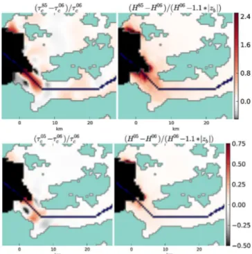
Figure 13 shows that the relative change in inferredτcis much more localized to the trough than the relative change in height above floatation. A slight increase inτc is visible near the margins of fast flow. But the broad pattern is similar, confirming that the relative change in height above floata-tion accounts for most of the relative changes inτc. Also for shorter timescales and after the disintegration of the floating ice tongue (2005–2006) similar patterns of relative change are visible (Fig. 13). An increase in sliding due to more melt water at the base, for example, would lead to a spatial pattern of relative change distributed over the entire area of melt. Be-cause we do not see this spatial pattern related to melt area,
Fig. 13.Relative change in inferredτc(left) compared to the change
predicted by the Mohr–Coulomb parameterization used in PISM. Areas where the bed topography,zb, is above sea level are masked
out.
our results support the findings of Joughin et al. (2008a) that increase in seasonal melt is not the main driver of the ob-served speed-up.
Figure 14 shows how the relative change in inferred τc (LHS of Eq. 6) and the predicted relative change in height above floatation (RHS of Eq. 6) compare along the center-line. The relative changes in inferredτcare shown for a range of regularization parameters and ice softness. The relative change in height above floatation has a different qualitative shape, but falls within the envelope of regularization parame-ters. The choice of regularization parameter gives a large un-certainty in relative changes inτc, especially in the terminus area. Above we showed that there is a significant lowering in τc in the first leg, even when taking into account the uncer-tainties introduced by the parameter choices in the inversion. Figure 14 on the other hand, shows that these same uncer-tainties of the inversion method make it difficult to judge the validity of parameterizations forτc(Eq. 5).
0 1 2 3 4 5
Rel. change
a
1985 - 2006
α = 3α = 30
0 5 10 15 20 25
Distance from 2008 grounding line (km) 0
1 2 3 4 5
Rel. change
b
(τ85
c −τc06)/τc06
(H85−H06)
H06−1.1 ∗|z
b|
A = 2 ×10⁻²⁴Pa−3s−1
A = 3 ×10⁻²⁴Pa−3s−1
0.5 0.0 0.5 1.0 1.5c
2005 - 2006
α = 3 α = 300 5 10 15 20 25
Distance from 2008 grounding line (km) 0.5
0.0 0.5 1.0
1.5d (τ
05
c −τc06)/τc06
(H05−H06)
H06−1.1 ∗|z
b|
A = 2 ×10⁻²⁴Pa−3s−1
A = 3 ×10⁻²⁴Pa−3s−1
Fig. 14.Relative change in inferred τc along the centerline for a
range of regularization parameters (top) and ice softness (bottom). The red line shows the change in height above floatation predicted by the Mohr–Coulomb parameterization used in PISM.(a) com-pares years 1985 and 2006,(b)compares the years 2005 and 2006.
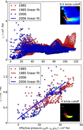
2006. When taking into account the entire misfit area, no re-lationship is apparent (Fig. 15), but when we limit the an-alyzed points to the areas of fast flow, a linear relationship emerges (Fig. 15). The slope of this linear fit indicates that tan(φ)≈0.02 and thusφ≈2◦, which is a very low value of till friction angle compared to the measured values between 19◦ and 26◦ (Iverson et al., 1998; Kamb, 1991). The con-sistent linear relationship in the fast flow area and the shift in data points to lower values are in agreement with the as-sumption of a constant tan(φ)in time. The unphysical value ofφand the lack of relationship betweenτcand the effective pressure over larger spatial scales, however, show that a sim-ple parameterization might not adequately represent the ac-tual bed properties under Jakobshavn Isbræ. In this study we use an approximation to a perfectly plastic sliding law,
there-Fig. 15.Inferredτcagainst effective pressure (ρgH−pw) for each
grid point where the observed velocities are greater than the thresh-old velocity given above the inset plots. A linear fit is given for both years, the slope is 0.016 (0.019) and the intercept is 1.37×10⁴Pa (0.97×10⁴Pa) for 1985 (2006).
physical parameters, but rather those that are consistent with a simplified physical model and the observations.
6 Conclusions
A careful choice of parameters in an inversion is especially important when comparing effective basal yield stress dis-tributions independently inferred for different years. To es-timate the influence of the parameter choices, reasonable ranges are explored and we find that the weakening of ef-fective basal yield stress over the years close to the terminus area is a real temporal variation. The observed changes are in agreement with a Mohr–Coulomb parameterization of effec-tive basal yield stress, where the change in effeceffec-tive pres-sure is the main driver for the changes in effective basal yield stress. Despite this broad agreement, the involvement of other processes cannot be excluded and the sensitivity of the inversion to parameter choices, in particular the regu-larization parameter, makes it difficult to evaluate effective basal yield stress parameterizations. The spatial distribution of residuals shows that for Jakobshavn Isbræ less simplified models, improved bed topography and/or a spatially varying ice softness could potentially improve the inversion results. With the currently available satellite data and the length of observational record on many other fast changing glacier sys-tems it is possible to apply these methods to other syssys-tems and to further advance our understanding of the changes at the base of the ice.
Acknowledgements. This work was supported by NASA NNX09AJ38G, NSF CMG 0732602, NSF CMG 0724860, and in part by a UAF Center for Global Change Student Research Grant with funds from the Cooperative Institute for Alaska Research and the UAF Vice Chancellor for Research, and Alaska EPSCoR. We acknowledge the use of data and data products from CReSIS generated with support from NSF grant ANT-0424589 and NASA grant NNX10AT68G, as well as Joughin et al. (2010). MEaSUREs Greenland Ice Velocity Map from InSAR Data. Boul-der, Colorado, USA: National Snow and Ice Data Center. Digital media. Ian Howat acted as scientific editor and two anonymous reviewers provided detailed comments that greatly improved the manuscript. Mark Fahnestock, Constantine Khroulev, Andy Aschwanden and Ed Bueler have patiently answered questions and provided feedback.
Edited by: I. M. Howat
References
Amundson, J. M., Fahnestock, M. A., Truffer, M., Brown, J., Lüthi, M. P., and Motyka, R. J.: Ice mélange dynamics and im-plications for terminus stability, Jakobshavn Isbræ, Greenland, J. Geophys. Res., 115, F01005, doi:10.1029/2009JF001405, 2010.
Aster, R. C., Borchers, B., and Thurber, C. H.: Parameter Estimation and Inverse Problems, ISBN 0120656043, Elsevier Academic Press, New York, 2005.
Bamber, J. L., Layberry, R., and Gogineni, S.: A new ice thickness and bed data set for the Greenland ice sheet. 1. Measurement, data reduction, and errors, J. Geophys. Res., 106, 33773–33780, 2001.
Budd, W. F. and Jacka, T. H.: A review of ice rheology for ice sheet modelling, Cold Reg. Sci. Technol., 16, 107–144, 1989. Bueler, E. and Brown, J.: Shallow shelf approximation as a “sliding
law” in a thermomechanically coupled ice sheet model, J. Geo-phys. Res., 114, F03008, doi:10.1029/2008JF001179, 2009. Calvetti, D., Morigi, S., Reichel, L., and Sgallari, F.: Tikhonov
regu-larization and the L-curve for large discrete ill-posed problems, J. Comput. Appl. Math., 123, 423–446, 2000.
Cuffey, K. M. and Paterson, W.: The Physics of Glaciers, 4 Edn., Academic Press, Amsterdam, 2010.
Gillet-Chaulet, F., Gagliardini, O., Seddik, H., Nodet, M., Du-rand, G., Ritz, C., Zwinger, T., Greve, R., and Vaughan, D. G.: Greenland ice sheet contribution to sea-level rise from a new-generation ice-sheet model, The Cryosphere, 6, 1561–1576, doi:10.5194/tc-6-1561-2012, 2012.
Habermann, M.: Basal shear strength inversions for ice sheets with an application to Jakobshavn Isbrae, Greenland, University of Alaska, Fairbanks, 2013.
Habermann, M., Maxwell, D., and Truffer, M.: Reconstruction of basal properties in ice sheets using iterative inverse methods, J. Glaciol., 58, 795–807, 2012.
Hansen, P. C.: The L-curve and its use in the numerical treatment of inverse problems, Computational inverse problems in electrocar-diology, 5, 119–142, 2001.
Iverson, N. R., Hooyer, T. S., and Baker, R. W.: Ring-shear stud-ies of till deformation: coulomb-plastic behavior and distributed strain in glacier beds, J. Glaciol., 44, 634–642, 1998.
Jay-Allemand, M., Gillet-Chaulet, F., Gagliardini, O., and Nodet, M.: Investigating changes in basal conditions of Variegated Glacier prior to and during its 1982–1983 surge, The Cryosphere, 5, 659–672, doi:10.5194/tc-5-659-2011, 2011.
Joughin, I., MacAyeal, D. R., and Tulaczyk, S.: Basal shear stress of the Ross ice streams from control method inversions, J. Geophys. Res., 109, B09405, doi:10.1029/2003JB002960, 2004.
Joughin, I., Das, S. B., King, M. A., Smith, B. E., Howat, I. M., and Moon, T.: Seasonal speedup along the western flank of the Greenland ice sheet, Science, 320, 781–783, 2008a.
Joughin, I., Howat, I. M., Fahnestock, M. A., Smith, B. E., Kra-bill, W. B., Alley, R. B., Stern, H., and Truffer, M.: Continued evolution of Jakobshavn Isbrae following its rapid speedup, J. Geophys. Res., 113, F04006, doi:10.1029/2003JB002960, 2008b.
Joughin, I., Tulaczyk, S., Bamber, J. L., Blankenship, D., Holt, J. W., Scambos, T., and Vaughan, D. G.: Basal conditions for Pine Island and Thwaites Glaciers, West Antarctica, deter-mined using satellite and airborne data, J. Glaciol., 55, 245–257, 2009.
Joughin, I., Smith, B. E., Howat, I. M., Scambos, T., and Moon, T.: Greenland flow variability from ice-sheet-wide velocity map-ping, J. Glaciol., 56, 415–430, 2010.
vari-ations in the surface velocity of Jakobshavn Isbrae, Greenland: observation and model-based analysis, J. Geophys. Res., 117, F02030, doi:10.1029/2011JF002110, 2012.
Julian, B. R. and Foulger, G. R.: Time-dependent seismic tomogra-phy, Geophys. J. Int., 182, 1327–1338, 2010.
Kamb, B.: Rheological nonlinearity and flow instability in the de-forming bed mechanism of ice stream motion, J. Geophys. Res., 96, 16585–16595, 1991.
Konovalov, Y. V.: Inversion for basal friction coefficients with a two-dimensional flow line model using Tikhonov regularization, Res. Geophys., 2, 82–89, 2012.
Korona, J., Berthier, E., Bernard, M., Rémy, F., and Thouvenot, E.: SPIRI T. SPOT 5 stereoscopic survey of polar ice: reference im-ages and topographies during the fourth international polar year (2007–2009), ISPRS J. Photogramm., 64, 204–212, 2009. Lüthi, M., Funk, M., Iken, A., Gogineni, S., and Truffer, M.:
Mech-anisms of fast flow in Jakobshavn Isbrae, West Greenland: Part 3: Measurements of ice deformation, temperature and cross-borehole conductivity in cross-boreholes to the bedrock, J. Glaciol., 48, 369–385, 2002.
MacAyeal, D. R.: The basal stress distribution of Ice Stream E, Antarctica, inferred by control methods, J. Geophys. Res., 97, 595–603, 1992.
Maxwell, D., Truffer, M., Avdonin, S., and Stuefer, M.: An iter-ative scheme for determining glacier velocities and stresses, J. Glaciol., 54, 888–898, 2008.
Meier, M. and Post, A.: Fast tidewater glaciers, J. Geophys. Res.-Sol. Ea., 92, 9051–9058, 1987.
Morland, L. W.: Unconfined ice-shelf flow, in: Dynamics of the West Antarctic ice sheet, edited by Van Der Veen, C. J., and Oerlemans, J., 99–116 pp., D. Reidel Publishing Company, Dor-drecht, 1987.
Morlighem, M., Rignot, E., Seroussi, H., Larour, E., Dhia, H. B., and Aubry, D.: Spatial patterns of basal drag inferred using con-trol methods from a full Stokes and simpler models for Pine Is-land Glacier, West Antarctica, Geophys. Res. Lett., 37, L14502, doi:10.1029/2010GL043853, 2010.
Motyka, R. J., Fahnestock, M., and Truffer, M.: Volume change of Jakobshavn Isbrae, West Greenland: 1985–1997–2007, J. Glaciol., 56, 635–646, 2010.
Motyka, R. J., Truffer, M., Fahnestock, M., Mortensen, J., Rysgaard, S., and Howat, I.: Submarine melting of the 1985 Jakobshavn Isbræ floating tongue and the trigger-ing of the current retreat, J. Geophys. Res., 116, F01007, doi:10.1029/2009JF001632, 2011.
Munson, T., Sarich, J., Wild, S., Benson, S., and Curf-man McInnes, L.: TAO 2.1 Users Manual, Tech. Rep. ANL/MCS-TM-322, 2012.
Payne, A. J., Vieli, A., Shepherd, A. P., Wingham, D. J., and Rig-not, E.: Recent dramatic thinning of largest West Antarctic ice stream triggered by oceans, Geophys. Res. Lett., 31, L23401, doi:10.1029/2004GL021284, 2004.
Petra, N., Zhu, H., Stadler, G., Hughes, T. J. R., and Ghattas, O.: An inexact Gauss–Newton method for inversion of basal sliding and rheology parameters in a nonlinear Stokes ice sheet model, J. Glaciol., 58, 889–903, 2012.
Pfeffer, W. T.: A simple mechanism for irreversible tide-water glacier retreat, J. Geophys. Res., 112, F03S25, doi:10.1029/2006JF000590, 2007.
Plummer, J., Gogineni, S., Van Der Veen, C. J., Leuschen, C., and Li, J.: Ice thickness and bed map for Jakobshavn Isbræ, CReSIS, Tech. rep., 2008.
Podlech, S. and Weidick, A.: A catastrophic break-up of the front of Jakobshavn Isbrae, West Greenland, 2002/03, J. Glaciol., 50, 153–154, 2004.
Raymond, M. J. and Gudmundsson, G. H.: Estimating basal properties of ice streams from surface measurements: a non-linear Bayesian inverse approach applied to synthetic data, The Cryosphere, 3, 265–278, doi:10.5194/tc-3-265-2009, 2009. Rignot, E. and Kanagaratnam, P.: Changes in the velocity structure
of the Greenland ice sheet, Science, 311, 986–990, 2006. Schoof, C. G. and Hindmarsh, R. C.: Thin-film flows with wall slip:
an asymptotic analysis of higher order glacier flow models, Q. J. Mech. Appl. Math., 63, 73–114, 2010.
Sohn, H.-G., Jezek, K. C., and Van Der Veen, C. J.: Jakobshavn Glacier, West Greenland: 30 years of spaceborne observations, Geophys. Res. Lett., 25, 2699–2702, 1998.
Thomas, R. H., Abdalati, W., Frederick, E., Krabill, W. B., Man-izade, S., and Steffen, K.: Investigation of surface melting and dynamic thinning on Jakobshavn Isbrae, Greenland, J. Glaciol., 49, 231–239, 2003.
Truffer, M.: The basal speed of valley glaciers: an inverse ap-proach, J. Glaciol., 50, 236–242, 2004.
Truffer, M. and Fahnestock, M.: Rethinking ice sheet time scales, Science, 315, 1508–1510, 2007.
Van Der Veen, C. J., Plummer, J., and Stearns, L.: Controls on the recent speed-up of Jakobshavn Isbræ, West Greenland, J. Glaciol., 57, 770–782, 2011.
Vogel, C. R.: Computational Methods for Inverse Problems, vol. 23, SIAM Series Frontiers in Applied Mathematics, Philadelphia, 1987.